YOLO11-Driven Deep Learning Approach for Enhanced Detection and Visualization of Wrist Fractures in X-Ray Images

Abstract

Wrist fractures, especially those involving the elbow and distal radius, are the most common injuries in children, teenagers, and young adults, with the highest occurrence rates during adolescence. However, the demand for medical imaging and the shortage of radiologists make it challenging to ensure accurate diagnosis and treatment. This study explores how AI-driven approaches are used to enhance fracture detection and improve diagnostic accuracy. In this paper, we propose the latest version of YOLO (i.e., YOLO11) with an attention module, designed to refine detection correctness. We integrated attention mechanisms, such as Global Attention Mechanism (GAM), channel attention, and spatial attention with Residual Network (ResNet), to enhance feature extraction. Moreover, we developed the ResNet_GAM model, which combines ResNet with GAM to improve feature learning and model performance. In this paper, we apply a data augmentation process to the publicly available GRAZPEDWRI-DX dataset, which is widely used for detecting radial bone fractures in X-ray images of children. Experimental findings indicate that integrating Squeeze-and-Excitation (SE_BLOCK) into YOLO11 significantly increases model efficiency. Our experimental results attain state-of-the-art performance, measured by the mean average precision (mAP50). Through extensive experiments, we found that our model achieved the highest mAP50 of 0.651. Meanwhile, YOLO11 with GAM and ResNet_GAM attained a maximum precision of 0.799 and a recall of 0.639 across all classes on the given dataset. The potential of these models to improve pediatric wrist imaging is significant, as they offer better detection accuracy while still being computationally efficient. Additionally, to help surgeons identify and diagnose fractures in patient wrist X-ray images, we provide a Fracture Detection Web-based Interface based on the result of the proposed method. This interface reduces the risk of misinterpretation and provides valuable information to assist in making surgical decisions.

1. Introduction

The human body has 206 bones, each varying in size, shape, and complexity. The smaller bones are placed in the ear canal, while the biggest are the femurs. Wrist fractures are the most common injuries people experience [1]. Wrist fracture injuries total approximately 2.7 million cases reported annually [2]. Occurrence typically reaches its greatest point at a young age [3,4,5,6]. They can lead to serious effects, including permanent damage, or even death [7]. Unfortunately, this type of injury is increasing commonly worldwide, even in the wealthiest countries, emphasizing the need to use advanced technologies to enhance detection and treatment. Wrist fractures are often from falls, accidents, physical altercations, and other incidents that affect individuals of all ages [8,9]. For this reason, timely and accurate diagnosis is essential for successful treatment. If a doctor or radiologist considers a cleavage, they usually order an X-ray to estimate the category and hardness of the fracture break [10].

Once wrist X-rays are obtained, they are usually clarified by physicians, including surgeons and medical trainees, to diagnose abnormalities. However, accurate assessment of these injuries can be a challenging task, particularly for healthcare professionals who lack specialized training in radiographic analysis. In many cases, physicians may have to make evaluations on their own without the help of expert radiologists or experienced colleagues, which can affect the accuracy of their diagnosis [11]. Health professionals have a huge responsibility, as they need to review thousands of X-ray images every day. When it comes to identifying wrist fractures, radiologists can sometimes become fatigued from analyzing such a large volume of images, which can lead to mistakes, or even missing a fracture that appears normal. However, manually examining X-rays for fractures is often slow, ineffective, and prone to mistakes. Unfortunately, many hospitals lack qualified CT scan experts to manage this workload effectively [12].

Studies indicate that diagnostic errors in the interpretation of emergency radiographs can reach rates as high as 26% [13,14,15]. This issue is increasing the global shortage of X-ray professionals, which persists even in established healthcare systems [16,17,18], and the limited availability of practitioners reporting in many regions worldwide presents a considerable risk to patient care [19]. The rising gap between the growing need for medical imaging studies and the constrained expansion of radiology placement programs is expected to further intensify this shortage. While the number of diagnosed image studies increases at an annual rate of approximately 5%, the growth in radiology residency positions remains limited to 2%, further burdening healthcare infrastructure [20]. Advanced imaging approaches, such as CT, MRI, and ultrasound, can supplement radiographic evaluation and upgrade the detection of wrist defects; however, certain fractures may remain unseen despite these additional techniques [21,22]. Recent advancements in computer vision (CV), particularly in object detection, have demonstrated significant capability in medical imaging. Recent studies have shown promising results in using automation to detect issues in trauma X-rays, indicating that artificial intelligence could improve diagnostic accuracy and help with clinical decision-making [23,24].

Computer-assisted diagnosis (CAD) in medical imaging serves acts as a valuable tool for MRI/CT scan experts, surgeons, and other healthcare professionals, assisting in complex decision-making processes. With continuous advancements in deep learning and the refinement of medical image processing approaches [25], there has been increasing interest in leveraging neural networks for CAD applications, including the detection of fractures [26,27,28,29]. These systems help diagnostic consultants detect wrist fractures more efficiently and accurately, providing valuable support to medical professionals in their work [30,31,32] Among the key developments in neural network-based CAD is the combination of attention mechanisms, which exceed the model’s expertise to focus on relevant input features. These mechanisms are broadly categorized into spatial attention, which captures pixel-level pairwise relationships, and channel attention, which models dependencies across different feature channels [33,34]. Research has demonstrated that incorporating attention mechanisms into convolutional neural networks (CNNs) can significantly raise performance in medical image analysis tasks [35].

AI-based methods have achieved both high accuracy and real-time performance in wrist fracture detection, but challenges remain. Deep learning approaches for automated object detection have arrived as possible solutions. Among these, the You Only Look Once (YOLO) series of models has gained attention for its real-time capabilities and enhanced accuracy in detecting and localizing objects [36]. The latest model YOLO11 [37], introduced by Ultralytics in 2024, has further outperformed the efficiency and accuracy of the object detection function of the GRAZPEDWRI-DX dataset [38], containing 20,327 pediatric wrist damage X-ray images, serving as a benchmark for evaluating fracture detection models. This study builds upon previous work, which assessed the efficiency of many neural network architectures on a given dataset, aiming to advance automated enhanced diagnostics in fracture detection.

Experimental results [39] show that combining a Residual Network (ResNet) [40] with the Global Attention Mechanism (GAM) extensively enhances the model performance. GAM first implements global pooling to collect high-level contextual information and then refines attention across spatial and channel dimensions for effective detection of fractures in medical images. ResNet improves feature extraction by measuring images at multiple scales. To leverage these benefits, we introduce ResNet_GAM, which merges both modules into the YOLO11 architecture to enhance feature analyzing and fracture detection. This method helps decrease false negatives, improves detection across various wrist regions, and raises the model’s stability in real-world clinical settings. After appraising various attention mechanisms, our results validate that this combination significantly improves feature representation, enhances fracture localization, and eliminates the limitations of traditional deep-learning approaches in medical imaging.

Contribution

• This study confirms that, compared to the YOLO11 baseline model, the performance of the YOLO11_GAM and ResNet_GAM models shows significant improvement in the GRAZPEDWRI-DX dataset.
• The integration of ResNet_GAM outperforms YOLO11_GAM, demonstrating that ResNet enhances feature extraction capabilities, leading to superior model accuracy.
• Additionally, we explore the use of Squeeze-and-Excitation (SE_BLOCK) in the Backbone part of the architecture, providing a further comparative analysis of attention-based enhancement in convolutional neural networks (CNN) feature learning.
• Section 2 presents an existing study on fracture detection using deep learning and explores the role of attention mechanisms in CNN architectures. Section 3 details the proposed YOLO11_GAM and ResNet_GAM model, along with the SE_Block enhanced architecture used in comparative studies. Section 4 provides a performance analysis of different models, comparing YOLO11_GAM, ResNet_GAM, and the SE_BLOCK-based approach against the baseline YOLO11 model. Section 5 discusses the impact of GAM on fracture detection accuracy, highlights the benefits of combining ResNet with GAM and analyzes the capability of ResNet with the SE_BLOCK in the ablation study. Section 6 concludes this research and overviews future directions.

2. Related Work

Medical image processing (MIP) is mostly used to detect wrist bone displacement. In the field of medical imaging, accuracy is very important because it directly affects the outcome. One-stage detectors are not always accurate enough for detailed tasks, so two-stage detectors are preferred for more complex cases. Building a high-quality fracture image is difficult because doctor’s annotations can vary. This makes it hard to create a standard system. As a result, deep learning models often focus on specific fracture types. There is a need for models that can detect fractures across various images and positions [41].

2.1. Transforming Medical Imaging with Deep Learning

This study shows that deep learning can outperform traditional methods in detecting wrist bone fractures. Switching from old methods to deep learning has made detection more precise and efficient. It also helps develop better and more reliable diagnostic tools for the future. Research in deep learning for MIP [42] shows that these models can be as effective as healthcare experts in diagnosis. Studies have shown that RNN and CNN models [43] can correctly diagnose Non-Small Cell Lung Cancer (NSCLC) outcomes, proving deep learning’s ability in cancer treatment. Additionally, deep learning has been applied in medical imaging fields, like pathology and chest CT detection, demonstrating rapid advancements. This highlights how computer vision and deep learning can enhance patient care in clinical settings [44].

2.2. Fracture Detection

These days, detecting wrist bone fractures is a main concern in medical imaging research. With deep learning, detection has shifted from basic image processing to advanced neural networks [45]. This section highlights deep-learning approaches for fracture detection, particularly in orthopedics and trauma care [28]. Studies show that deep learning models effectively identify fractures, improving diagnosis and treatment. Their success in classifying fractures in X-ray images demonstrates their capacity to upgrade accuracy and efficiency in medical imaging [46]. Additionally, deep learning has also been used to measure wrist bone density and measure fracture risk [23], showing its ability to examine bone health. Researchers have even developed a new model for detecting ulnar fractures, leading to more specialized applications in fracture detection. Further progress in this area is made possible by combining a unique CNN way with an enhanced canny edge detection algorithm to optimize fracture analysis [47].

2.3. YOLO-Based Deep Learning Models

Work connecting deep learning and machine learning highlighting the ongoing developments in technology within this field [41]. Fracture detection has emerged as an important topic in MIP. Numerous neural networks have been employed for this task, with the YOLO family, including YOLOv5 [48], gaining particular prominence. For instance, YOLOv5 was used to identify regions of fractures in 704 child healthcare chest X-ray (CXR) pictures [49]. Combined data augmentation with YOLOv5 has been used to detect fractures in CXR datasets [50]. The classification of facial jaw fractures into four types, i.e., as frontal, midfacial, mandibular, and no fracture, employed YOLOv5 to classify them in 3407 CT images. In a related study, YOLOv5 was used to diagnose mandibular fractures from X-ray images [51]. The external attention and 3D feature fusion methods were employed using YOLOv5 for skull CT fracture detection [52]. Furthermore, vertebral localization is considered vital in identifying vertebral deformities and fractures; for example, YOLOv5 is used to localize lumbar vertebrae with a mean average precision (mAP) of 0.957 [53]. Although YOLOv5 has been widely adopted for fracture detection, the use of YOLOv8 [37] remains relatively limited in comparison.

New advancements in one-stage detection algorithms along with advanced YOLO models have a limited accuracy interval. The option between one and two-stage detectors finally depends on the task’s exact requirements, with the main focus on achieving excellent accuracy. YOLO models [54] break an image into small square grids. Each grid predicts object locations by estimating the position of bounding boxes using a regression-based method. Object detection can involve thousands of possible bounding boxes, which makes the process computationally heavy to simplify. YOLO models use anchor boxes with predefined shapes and sizes on each grid cell to help identify objects. This approach enables the detection of various objects but also increases computational load and slows processing speed. Different researchers have developed numerous models for fracture detection. A review provides an overview of these techniques [55]. According to [56], fracture detection and localization are often carried out using various versions of YOLO algorithms. These models differ depending on the specific body area being examined and the particular YOLO model applied.

2.4. Two-Stage Detection

Two-stage models are widely used for object detection, but some studies have explored single-stage detectors for fracture classification. For example, in [57], researchers applied the YOLOv2 model to detect spinal fractures from CT scans. They worked with a dataset of 5134 CT scans from Xijing, a Chinese hospital, and trained an enhanced version of YOLOv2 for this purpose. Their model accomplishes a means average precision (mAP@0.5) and Intersection over Union (IoU) of 0.773, demonstrating effective performance in fracture detection. Researchers have also improved CT image skull fracture detection by combining external attention with 3D features. A machine learning model using the YOLOv4 technique showed that it could outperform MRI specialists and enrich prediction accuracy [58]. Two-stage bone fracture detection systems often use transfer learning by fine-tuning existing models, particularly those based on Regions with Convolutional Neural Networks (R-CNN) [59] and Faster Region Proposal Networks (Faster RPN) [30]. The RPN uses a CNN to first recognize possible regions where any instances of objects of attention may be situated in the input image, and then only retains the High-certainty regions. A Faster R-CNN model with a VGG16 backbone was used to detect fracture of the distal radius in front-view wrist X-ray images. The model performed well, obtaining a mAP of (0.87) on a test set of 1312 x-ray images. Its value was not in the fact that the original dataset had only 95 pictures (both fractured and non-fractured), but that these were increased using data augmentation techniques to make a larger set for training and testing [60]. Two different Faster R-CNN models, each using Inception and ResNet, were trained to detect wrist fractures, one for front-view (frontal) X-rays and one for side-view (lateral) X-rays. The frontal model was trained on 6515 images, while the lateral model used 6537 images. The front view model correctly identified 91% of fractures, with 83% accuracy and 96% sensitivity. The lateral model executed marginal improvements, detecting fractures inn 96% of cases, with a specificity of 86% and a sensitivity of 97%. Both models displayed strong overall performance, with high AUC–ROC scores: 0.92 for the frontal model and 0.93 for the lateral model. When observing the combined results per patient study, the models Achieved a specificity of 73%, a sensitivity of 98%, and an AUC–ROC of 0.89 [61].

2.5. Attention Module

SENet [51], introduced a pioneering mechanism for learning channel attention by independently executing Global Average Pooling (GAP) to every channel. Afterwards, channel weights were created via the sigmoid function and fully connected layers, resulting in improved model performance. Building on SENet, feature aggregation, and recalibration strategies, several studies [62,63,64] attempted to refine the SE_BLOCK to better capture channel-wise dependencies. Meanwhile, the integrated channel attention with spatial attention in the CBAM module enriches CNN representation capabilities [46]. To reduce information loss and emphasize cross-dimensional features, CBAM was extended by proposing GAM, which reconfigured its submodules to highlight relevant multi-dimensional receptive fields [65]. Although these attention mechanisms yielded higher accuracy, they also introduced greater complexity and computational overheads. In response, Enhanced Convolutional Attention (ECA) [66], developed a module that exploits local cross-channel interactions by regarding each channel in conjunction with its k-nearest neighbors, achieving strong performance gains with fewer parameters. In contrast, the Self-Attention (SA) [67] module proposed that channel dimension is divided into multiple sub-features; each sub-feature is then processed with a shuffle unit to combine complementary components with a spatial attention mechanism, leading to excellent results and reduced complexity [39].

2.6. Identified Gaps and Study Motivation

Despite broad research on deep learning for wrist fracture detection, presented models still face significant challenges that limit their complete performance. An important limitation is partial detection, as the majority of models are trained on specific wrist regions to reduce their adaptability to many fracture locations. Additionally, fluctuations in image resolution lead to diverse performance across different datasets. Existing studies have integrated attention mechanisms and ResNet for improved feature extraction in medical imaging, combined with YOLO11 to improve wrist fracture detection. Another crucial challenge is ineffective feature extraction, where the oldest models’ efforts to capture fundamental fracture features often result in misclassifications or missed detections. ResNet_GAM enhances feature extraction, enabling the model to identify even minor fractures with higher accuracy. Furthermore, many existing models lack attention-based mechanisms, inducing them to overlook key regions in X-ray images. To minimize this problem, we implement an SE_BLOCK between the Backbone and Neck, ensuring refined feature collection and improved focus on fracture-prone areas, ultimately enhancing detection reliability.

3. Material and Methods

3.1. Model Architecture

YOLO11 is our baseline model, which consists of backbone, neck, and head, as displayed in Figure 1. In the latest model of the YOLO series, YOLO11 developed by Ultralytics, a significantly advanced architecture boosts training efficiency and processing speed and retains high accuracy with fewer parameters. In YOLOv8, the backbone architecture includes the C2f (C2 Focus), an improved version of the CSP (Cross-Stage Partial) module. However, in the transition from YOLOv8 to YOLO11, the C2f block was replaced with the C2K3 block. Unlike C2f, the C2K3 block in YOLO11 replaces the bottleneck structure with stacked 3 × 3 convolutions aimed at improving feature extraction, expanding the receptive field, and enhancing small object detection. This novel block configuration utilizes dual smaller convolutions within the framework of the CSP Bottleneck, optimizing both computational efficiency and model throughput without sacrificing detection precision. The YOLO11 model has five scalable versions ranging from nano to extra-large, designed to accommodate diverse computational and correctness requirements across various deployment scenarios. An important enhancement in YOLO11 is the integration of the Cross-Stage Partial with Self-Attention (C2PSA) module. This module smartly merges the architectural efficiencies of cross-stage partial networks with the contextual sensitivity of self-attention mechanisms.

3.2. Backbone

The Backbone is the primary phase of the YOLO11 model, responsible for extracting multi-scale features from the input image. It includes convolutional layers, C3K2 blocks, Spatial Pyramid Feature Fusion (SPFF), and Channel and Spatial Attention (C2PSA). These elements capture low-level and high-level features, which are subsequently processed by the Neck and Head for object detection:

$$\mathrm{X}\in {\mathbb{R}}^{\mathrm{H}\times \mathrm{W}\times \mathrm{C}}$$

(1)

where X represents an image, ℝ denotes a real number, and H, W, and C correspond to the height, width, and number of channels of the images. The channel can be RGB for color and/or Grayscale for X-ray images.

3.2.1. Convolutional Layers (Conv)

The first two layers are convolutional layers (Conv), which process the input using a linear transformation and applied non-linear activation function. This helps the network extract significant patterns and advance its capability to make accurate predictions:

$$\mathrm{Z}=\mathrm{F}\times \mathrm{X}+\mathrm{b}$$

(2)

$${\mathrm{Y}}^{\prime }=\mathsf{\sigma }\left(\mathrm{Z}\right)$$

(3)

where F is used as a filter of the convolutional kernel, and b is used as a bias term that works with weights to adjust the output. σ acts as an activation function (e.g., ReLU or Sigmoid) and adds nonlinearity. Z is the output of the pre-activation. Finally, Y′ represents the final processed output.

3.2.2. C3K2 Blocks (CSP Bottleneck with Kernel Size 2)

YOLO11 replaces the C2F block with C3k2 blocks, which are significantly faster and more effective than the C2F. A C3K2 Block comprises three convolutional layers with a kernel size of two refining image representations. The equation below enables the Backbone to extract layered features from the input image:

$$\mathrm{Z}={\mathrm{U}}_3\times \left(\mathsf{\sigma }\left({\mathrm{U}}_2\times \left(\mathsf{\sigma }\left({\mathrm{U}}_1\times \mathrm{X}+{\mathrm{b}}_1\right)\right)+{\mathrm{b}}_2\right)\right)+{\mathrm{b}}_3$$

(4)

This process can be described as a multi-layer transformation, where the input image (i.e., X) passes through convolutional layers and each layer applies with weights (i.e., U₁, U₂, U₃) and biases (i.e., b₁, b₂, b₃), followed by an activation function ($\mathsf{\sigma })$, and finally producing the final output transformed feature map (i.e., Z) after processing through all the layers.

3.2.3. Residual Connections (Shortcut = False, n = 3 $\times$ d)

A residual connection or skip connection is a method used in deep neural networks, especially in ResNet, to enhance gradient flow, stabilize training, and enable deeper architectures. For residual connections, if a shortcut is false, the residual connection is removed:

$${\mathrm{Y}}_{\mathrm{o}\mathrm{u}\mathrm{t}}=\mathrm{F}\left(\mathrm{X}\right)$$

(5)

where (X) is the input feature map, F(X) is the feature transformation using convolutional layers, and Y_out is the final output without adding X.

3.2.4. Residual Connections (Shortcut = True, n = 6 × d)

When this is true, the model includes a residual connection, meaning the input X layer is directly passed to the output. This is the transformation function F(X). For residual connections, if shortcut is true:

$${\mathrm{Y}}_{\mathrm{o}\mathrm{u}\mathrm{t}}=\mathrm{F}\left(\mathrm{X}\right)+\mathrm{X}.$$

(6)

This directly connects the input to the output, allowing the model to learn an identity function, if necessary, which helps in reducing the vanishing gradient problem that arises when deep networks need to propagate gradients effectively throughout backpropagation. The residual direct connection gradient path increases deep network training efficiency.

3.3. Neck

The Neck part of YOLO11 combines multi-scale features from the Backbone and transmits them to the Head for final prediction. In object detection models, the Neck plays a key role in combining features from different scales, improving their quality through up-sampling, and refining them before passing data to the detection head. It refines and merges the feature maps from the Backbone, ensuring that critical information from various levels of the various features is retained. It includes several C3k2 modules arranged along different pathways to refine and process features at multiple scales and depths. After the C3k2 modules, the design uses multiple convolution modules, essential for further refinement of the features.

3.3.1. SPFF (Spatial Pyramid Feature Fusion)

The SPFF module helps boost object detection by executing several pooling operations to create feature pyramids. These feature pyramids ensure that both small and large structures in an image are effectively identified, leading to more accurate object detection. as follows:

$${\mathrm{Y}}_{\mathrm{S}\mathrm{P}\mathrm{F}\mathrm{F}}={\sum }_{\mathrm{s}\in \mathrm{S}}^{{\mathrm{P}}_{\mathrm{s}}}\mathrm{X}$$

(7)

where Ps(X) is a pooling operation applied at scale s and S represents multiple scales. This allows the model to preserve fine details while improving the detection of larger objects.

3.3.2. C2PSA (Channel and Spatial Attention)

A significant enhancement in YOLO11 is the C2PSA, placed after the SPPF block for spatial representation in feature maps. A sigmoid activation function is applied to calculate channel-specific significance, followed by spatial attention using a 7 × 7 convolution to highlight important features. Finally, the model channel attention (i.e., F_c) and spatial attention (i.e., F_s), lead to better feature optimization, as follows:

$${\mathrm{W}}_{\mathrm{c}}=\mathsf{\sigma }\left({\mathrm{F}}_{\mathrm{c}}\times \mathrm{G}\mathrm{A}\mathrm{P}\left(\mathrm{X}\right)\right)$$

(8)

$${\mathrm{W}}_{\mathrm{s}}=\mathsf{\sigma }\left({\mathrm{F}}_{\mathrm{s}}\times \mathrm{X}\right)$$

(9)

$${\mathrm{Z}}_{\mathrm{C}2\mathrm{P}\mathrm{S}\mathrm{A}}={\mathrm{W}}_{\mathrm{c}}\times \mathrm{X}+{\mathrm{W}}_{\mathrm{s}}\times \mathrm{X}$$

(10)

where F_c is the channel filter applied to the Global Average Pooled (GAP), and Fs is special attention directly applied to the input feature map (X) to compute spatial attention, which reduces the input feature map (i.e., X) to a single averaged value per channel. W_c, W_s, channel-wise, highlight the important channels in the feature map, and with special attention to weights that focus on important special locations.

3.3.3. Up-Sampling Operation

Up-sampling is a technique used in deep learning to increase the spatial resolution of a low-resolution feature map to match the resolution of a higher-resolution layer. This is essential for multi-scale feature fusion, where features from different levels of the network are combined:

$${\mathrm{Y}}_{\mathrm{u}\mathrm{m}\mathrm{s}\mathrm{a}\mathrm{m}\mathrm{p}\mathrm{l}\mathrm{e}}=\mathrm{U}\mathrm{p}\mathrm{s}\mathrm{a}\mathrm{m}\mathrm{p}\mathrm{l}\mathrm{e}(\mathrm{X},\mathrm{s}\mathrm{c}\mathrm{a}\mathrm{l}\mathrm{e}=2)$$

(11)

where X is the low-resolution feature map, the scale factor increases the height and width of X, and Y_upsample (X scale =2) doubles the height and width factor of 2. Y_upsample also enables high-resolution multi-scale fusion and improves object detection accuracy.

3.3.4. Concatenation of Feature Maps

Concatenation merges multiple feature maps from different levels (e.g., low-level and high-level features). This operation enhances feature representation by combining different spatial and conceptual details. After passing through C3K2 Blocks, the model concatenates feature maps from different levels:

$${\mathrm{Y}}_{\mathrm{c}\mathrm{o}\mathrm{n}\mathrm{c}\mathrm{a}\mathrm{t}}=\mathrm{C}\mathrm{o}\mathrm{n}\mathrm{c}\mathrm{a}\mathrm{t}({\mathrm{X}}_1,{\mathrm{X}}_2,{\mathrm{X}}_3\dots ,{\mathrm{X}}_{\mathrm{n}})$$

(12)

where Y_concat represents the final feature map after merging is obtained. The Concat denotes the concatenation process, with multiple input feature maps X₁, X₂, X₃, …, X_n.

3.3.5. ResNet_GAM

ResNet_GAM improves feature learning by emphasizing important spatial and channel-wise features. Concatenation merges multiple feature maps from different levels (e.g., low-level and high-level features). This method increases the model capacity to obtain relevant patterns while maintaining efficient training. In deep learning, very deep networks suffer from vanishing gradients, making effective training difficult. ResNet resolves this problem using skip connections (identity mapping) that allow gradients to flow smoothly. The residual learning equation in ResNet is:

$$\mathrm{Y}=\mathrm{F}\left(\mathrm{i},\mathrm{W}\right)+\mathrm{i}$$

(13)

where F (i, W) is the residual function and Y is the output of the Res_Block.

3.4. Head

This section deals with improving the detection produced by the Backbone and Neck. Highly accurate bounding boxes, class predictions, and confidence scores are predicted. Advanced attention mechanisms, well-feature fusion, and increased loss functions are mixed to deliver innovative performance in real-time object identification.

3.4.1. Feature Maps from the Neck to the Head

In the Neck, the features extracted from the Backbone go through several processes, like C3K2 blocks, Convolutions, and ResNet_GAM modules, which aim to refine the feature maps. After passing through the ResNet_GAM module, the feature maps are forwarded to the Head section for further processing as follows:

$${\mathrm{F}}_{\mathrm{N}\mathrm{e}\mathrm{c}\mathrm{k}}\in {\mathbb{R}}^{\mathrm{H}\times \mathrm{W}\times \mathrm{C}}$$

(14)

where F_Neck is a feature map generated by the Neck.

3.4.2. Detection (DETECT)

After passing through ResNet_GAM, the Head and DETECT modules generate bounding boxes to locate objects and predict their probabilities. The Head processes the refined feature maps (F_{Neck_out}) and applies another ResNet_GAM layer, further enhancing key features before making final predictions. The refined feature maps in the Head are denoted as F_h, as follows:

$${\mathrm{F}}_{\mathrm{h}}={\mathrm{A}}_{\mathrm{h}}\mathrm{ʘ}{\mathrm{F}}_{\mathrm{N}\mathrm{e}\mathrm{c}\mathrm{k}\_\mathrm{o}\mathrm{u}\mathrm{t}}$$

(15)

Here, A_h denotes the newly computed attention map for the Head. It is derived in a similar way as in the Neck, using a separate weight matrix W_h and bias term b_h: F_h as follows:

$${\mathrm{A}}_{\mathrm{h}}=\mathrm{s}\mathrm{o}\mathrm{f}\mathrm{t}\mathrm{m}\mathrm{a}\mathrm{x}({\mathrm{W}}_{\mathrm{h}}\times {\mathrm{F}}_{\mathrm{N}\mathrm{e}\mathrm{c}\mathrm{k}}+{\mathrm{b}}_{\mathrm{h}})$$

(16)

This refined feature map F_h is then passed to the final DETECT layers to make object detection predictions. The final object detection output from the DETECT layer is as follows:

$$\mathrm{Y}=\mathrm{D}\mathrm{E}\mathrm{T}\mathrm{E}\mathrm{C}\mathrm{T}\left({\mathrm{F}}_{\mathrm{h}}\right).$$

(17)

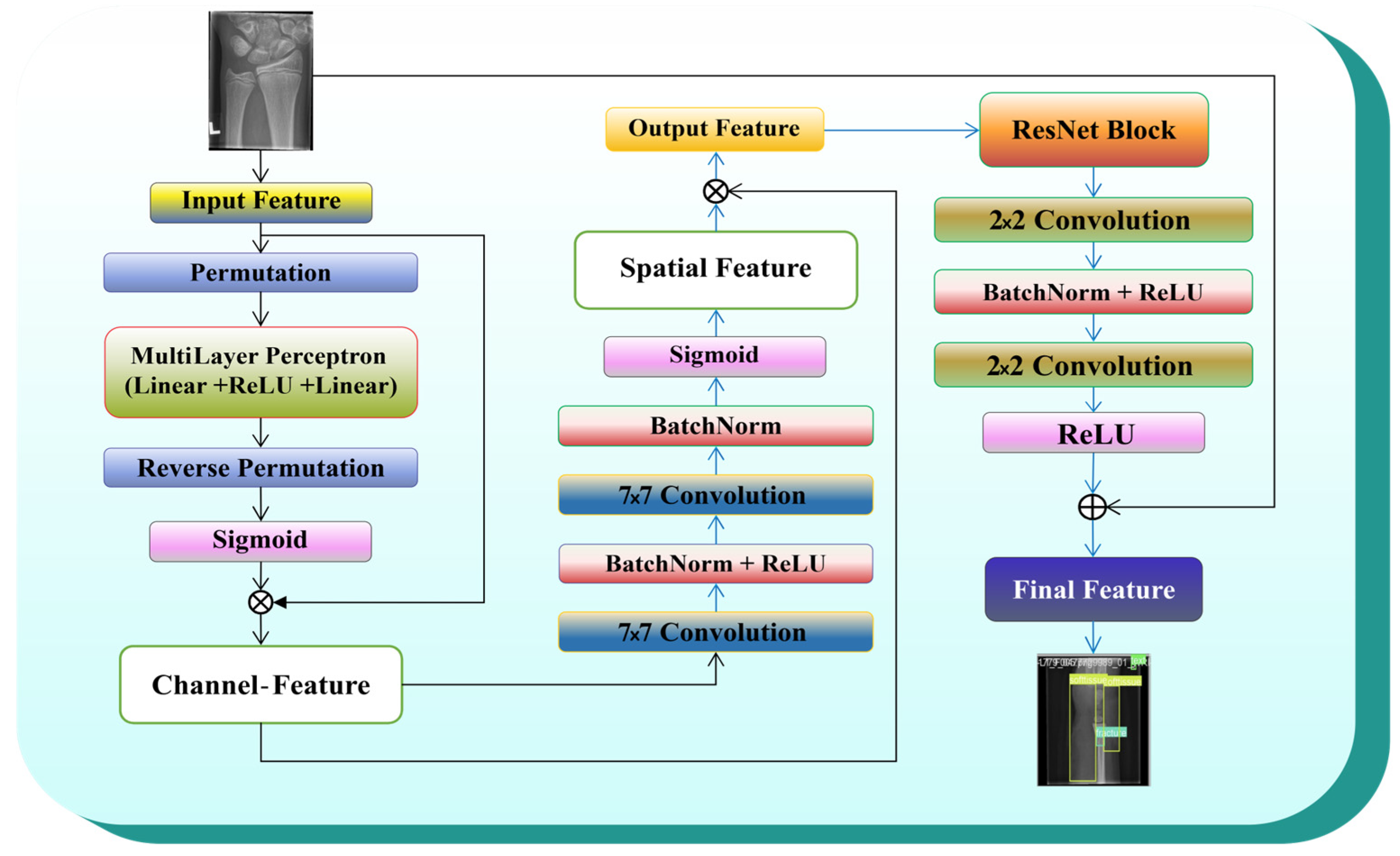
3.5. ResNet with GAM

This section aims at improving the detections produced by the Backbone and Neck. It creates highly accurate bounding boxes, class predictions, and confidence scores. It mixes advanced attention mechanisms, well-feature fusion, and increased loss functions to deliver innovative performance in real-time object identification. ResNet_GAM combines two advanced techniques to elevate deep learning models, particularly for object detection and image classification, as described in Figure 2. It boosts accuracy while improving computational efficiency enabling faster training, better adaptability, and reduced parameter usage compared to conventional models. Res_Block uses skip connections to maintain information flow and support deeper network training, addressing vanishing gradient issues for more effective learning. Meanwhile, GAM directs focus towards key regions in an image rather than treating all areas equally, making it especially beneficial for object detection.

3.5.1. Global Attention Mechanism (GAM)

The GAM refines the data and improves global feature interactions. It uses the spatial attention and sequential channel mechanisms from the Convolutional Block Attention Module (CBAM) but with redesigned submodules for better performance. In contrast to CBAM, the creators of GAM determined that max-pooling could diminish too much data and harm performance, so they removed pooling to better preserve the feature map. Additionally, we added the skip connection inside the GAM layers to this substance’s quicker input movement speed, as shown in the equation below:

$${\mathrm{F}}_{\mathrm{o}\mathrm{u}\mathrm{t}}={\mathrm{F}}_{\mathrm{i}\mathrm{n}}+\left[{\mathrm{M}}_{\mathrm{s}}\left({\mathrm{M}}_{\mathrm{c}}\left({\mathrm{F}}_{\mathrm{i}\mathrm{n}}\right)\otimes {\mathrm{F}}_{\mathrm{i}\mathrm{n}}\right)\otimes \left({\mathrm{M}}_{\mathrm{c}}\left({\mathrm{F}}_{\mathrm{i}\mathrm{n}}\right)\otimes {\mathrm{F}}_{\mathrm{i}\mathrm{n}}\right)\right]$$

(18)

where F_in and F_out signify the input and output feature maps, respectively. Meanwhile, M_c and M_s denote the channel and spatial attention mechanisms.

3.5.2. Channel Attention Mechanism (CAM)

The CAM ensures that the model focuses on the significant channels for the feature map rather than treating all feature maps equally. In CAM, GAM first uses a method to preserve three-dimensional (i.e., 3D) information. Then, a two-layer MLP is applied to spatial connections between channels at different scales. Rather than compressing the spatial dimensions (i.e., H × W) to obtain channel weights, it slightly reduces the channel dimension (i.e., C/r) to derive spatial weights. To summarize, the equation is

$${\mathrm{M}}_{\mathrm{c}}\left(\mathrm{P}\right)=\mathsf{\sigma }[\mathrm{R}\mathrm{e}\mathrm{v}\mathrm{e}\mathrm{r}\mathrm{s}\mathrm{e} \mathrm{P}\mathrm{e}\mathrm{r}\mathrm{m}\mathrm{u}\mathrm{t}\mathrm{a}\mathrm{t}\mathrm{i}\mathrm{o}\mathrm{n}\left(\mathrm{M}\mathrm{L}\mathrm{P}\left(\mathrm{P}\mathrm{e}\mathrm{r}\mathrm{m}\mathrm{u}\mathrm{t}\mathrm{a}\mathrm{t}\mathrm{i}\mathrm{o}\mathrm{n}\left(\mathrm{F}\right)\right)\right)]$$

(19)

where P is the reverse permutation of multi-layer perceptron (MLP) and F is the input feature map.

An MLP with two fully connected layers and ReLU activation is utilized. After applying the MLP, the result is reversed back to the original shape. A sigmoid activation normalizes the values between [0, 1] and channel attention map Ac is applied through element-wise multiplication with the input feature map, as follows:

$$\mathrm{M}={\mathrm{W}}_2\times \mathsf{\sigma }\left({\mathrm{W}}_1{\mathrm{X}}^{\prime }+{\mathrm{b}}_1\right)+{\mathrm{b}}_2$$

(20)

where X′ is the input feature map passed through an MLP with two fully connected layers. First layer: W₁X′ + b₁, followed by an activation function (ReLU or sigmoid σ). Second layer: W₂ × σ (activated output) + b₂.

3.5.3. Spatial Attention Mechanism (SAM)

SAM increases the features, depending on spatial location. This component emphasizes spatial information by employing two convolutional layers to integrate and refine the spatial characteristics of the feature map; since max pooling can reduce crucial feature details, it limits further feature extraction to preserve feature information. This submodule removes the pooling step, as follows:

$${\mathrm{S}}_1=\mathrm{R}\mathrm{e}\mathrm{L}\mathrm{U}\left(\mathrm{B}\mathrm{N}\right({\mathrm{W}}_{\mathrm{s}}^{\left(1\right)}\times \mathrm{X})$$

(21)

where X is the input feature map passed through a 7 × 7 convolutional layer with a ${\mathrm{W}}_{\mathrm{s}}^{\left(1\right)}$ filter. Batch Normalization (BN) is applied to stabilize the activations and the ReLU activation function is used for non-linearity:

$${\mathrm{S}}_2=\mathrm{R}\mathrm{e}\mathrm{L}\mathrm{U}\left(\mathrm{B}\mathrm{N}\right({\mathrm{W}}_{\mathrm{s}}^{\left(2\right)}\times {\mathrm{S}}_1)$$

(22)

where S₁ is the output from the first convolution layer, which undergoes another 7 × 7 convolution layer using ${\mathrm{W}}_{\mathrm{s}}^{\left(2\right)},$ and again BN and ReLU activation are applied.

3.5.4. Residual Block (ResNet_Block)

In ResNet_Block, first 3 × 3 convolutional layer features are extracted, followed by batch normalization to stabilize training of the applied ReLU activation function, then negative values are removed, ensuring non-linearity. A 1 × 1 convolution adjusts the feature map’s depth to match the input. The key element, a skip connection, directly links the input to the output, preventing data loss and addressing the vanishing gradient issue in deep networks. Finally, another ReLU activation refines the output before passing it to the next layer. In this process, deep networks learn effectively by preserving essential features, improving training efficiency, and maintaining performance as the network deepens. This can be stated as

$$\mathrm{Z}=\mathrm{f}\left(\mathrm{x},\left\{{\mathrm{w}}_{\mathrm{i}}\right\}\right)+\mathrm{x}$$

(23)

where f (x, {w_i}) signifies the learned transformation function that is applied to the original input x, which enters into the residual block. It contains features that are typically processed through a series of convolutional operations and transformation applies tangible weights {w_i}, which are updated during the training. Z is the final point of the Res_Block after adding the input and transformation.

3.6. Squeeze-and-Excitation (SE_BLOCK)

The SE_BLOCK is an advanced attention mechanism that improves feature representation in CNN, pointedly boosting image recognition performance, as displayed in Figure 3. In YOLO11, the SE_BLOCK is placed between the backbone and neck, fine-tuning features before passing them to the neck, which improves detection accuracy.

3.6.1. Squeeze (Global Information Embedding)

SE_BLOCK enhances spatial information by applying GAP to the feature maps instead of treating all channels uniformly. This transforms a W × H × C feature map into a 1 × 1 × C vector by compressing spatial dimensions while preserving channel information, summarizing the most essential information from all spatial locations, as follows:

$${\mathrm{Z}}_{\mathrm{k}}={\displaystyle \frac{1}{\mathrm{H}\times \mathrm{W}}}{\sum }_{\mathrm{X}=1,\mathrm{j}=1}^{\mathrm{H},\mathrm{W}}{\mathrm{X}}_{\mathrm{c}}(\mathrm{x},\mathrm{j})$$

(24)

where X_c (x, j) represents the activation of the feature map for the channel, C is the spatial location (x, j) and Z_k is the squeezed feature (scalar value per channel).

3.6.2. Excitation (Channel-Wise Attention)

SE_BLOCK learns channel dependencies by passing the squeezed vector delivered over a small neural network with two fully connected layers and activation functions to model interdependencies between channels. The weights that highlight important features and suppress less useful ones are as follows:

$${\mathrm{Z}}^{\prime }={\mathsf{\sigma }(\mathrm{F}\mathrm{C}}_2\left(\mathsf{\delta }\left({\mathrm{F}\mathrm{C}}_1\left(\mathrm{z}\right)\right)\right)).$$

(25)

The first layer (i.e., FC₁) projects z into a lower-dimensional space with a reduction factor r, while the second layer (i.e., FC₂) restores it to the original dimension. The final vector, Z′, shows how important each channel is, based on the current situation.

3.6.3. Rescale (Feature Recalibration)

After computing the attention weights, the original feature map is recalibrated. Channels with higher weights are enhanced, while less important ones are suppressed, leading to a more refined feature representation.

3.7. Evaluation Matrices

It is significant to assess the performance of an AI model using suitable evaluation metrics to ensure its reliability and effectiveness. In this experiment, we used popular evaluation metrics for the calculation of the proposed method.

3.7.1. FLOPs (Floating-Point Operations)

Computing systems use FLOPs as an evaluation standard because they provide a method to measure neural network model complexity. To determine the necessary computational power for pattern recognition in new datasets, the required quantity of FLOPs serves as a helpful estimation tool, as follows:

$${\mathrm{F}\mathrm{L}\mathrm{O}\mathrm{P}}_{\mathrm{S}}={\sum }_{i=1}^T{\mathrm{O}}_{\mathrm{i}}.$$

(26)

3.7.2. Intersection over Union (IoU)

The IoU calculation represents a ratio between overlapping areas and joint areas from predicted and true bounding boxes, thus measuring their spatial correspondence. The calculation is as follows:

$$\mathrm{I}\mathrm{o}\mathrm{U}={\displaystyle \frac{\mathrm{r}\mathrm{e}\mathrm{g}\mathrm{i}\mathrm{o}\mathrm{n}\left(\mathrm{A}\right)\cap \mathrm{r}\mathrm{e}\mathrm{g}\mathrm{i}\mathrm{o}\mathrm{n}\left(\mathrm{B}\right)}{\mathrm{r}\mathrm{e}\mathrm{g}\mathrm{i}\mathrm{o}\mathrm{n}\left(\mathrm{A}\right)\cup \mathrm{r}\mathrm{e}\mathrm{g}\mathrm{i}\mathrm{o}\mathrm{n}\left(\mathrm{B}\right)}}.$$

(27)

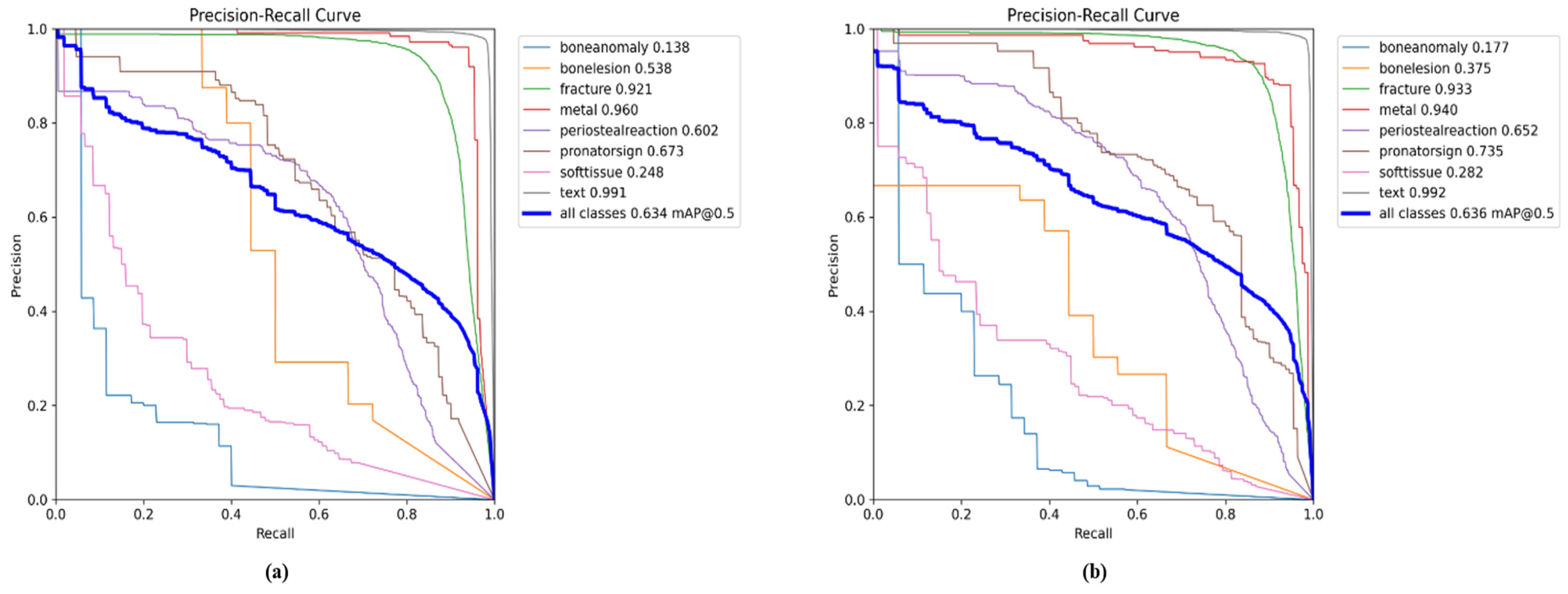
3.7.3. Precision–Recall Curve

The Precision–Recall curve shows values for recall along the x-axis while precision values are located on the y-axis. The equations determine the values of recall (i.e., R) and precision (i.e., P), as follows:

$$\mathrm{R}\mathrm{e}\mathrm{c}\mathrm{a}\mathrm{l}\mathrm{l}={\displaystyle \frac{\mathrm{T}\mathrm{P}}{\mathrm{T}\mathrm{P}+\mathrm{F}\mathrm{N}}}.$$

(28)

3.7.4. Mean Average Precision (mAP)

The mAP is the main metric for evaluating object detection models. It evaluates how well the model recognizes and positions objects using precision–recall curves. mAP is calculated in two ways: (1) mAP@0.5, which uses a fixed threshold, and (2) mAP@0.5:0.95, which analyzes across multiple thresholds for a more complete performance calculation. The equation of the metric is as follows:

$$\mathrm{m}\mathrm{A}\mathrm{P}={\displaystyle \frac{1}{N}}{\sum }_{i=1}^N\mathrm{A}\mathrm{P}\mathrm{i}.$$

(29)

3.7.5. F1-Score

The F1-score is a widely used metric for evaluating accuracy, as it effectively balances precision and recall. It is computed as the harmonic mean of precision and recall with values, ranging from 0 to 1. A higher F1 score approaching 1 indicates a good balance between precision and recall, whereas a score closer to 0 indicates poor performance due to low precision or recall. The equation of the metric is as follows:

$${\mathrm{F}}_1={\displaystyle \frac{2\times \mathrm{P}\mathrm{r}\mathrm{e}\mathrm{c}\mathrm{i}\mathrm{s}\mathrm{i}\mathrm{o}\mathrm{n}\times \mathrm{R}\mathrm{e}\mathrm{c}\mathrm{a}\mathrm{l}\mathrm{l}}{\mathrm{P}\mathrm{r}\mathrm{e}\mathrm{c}\mathrm{i}\mathrm{s}\mathrm{i}\mathrm{o}\mathrm{n}+\mathrm{R}\mathrm{e}\mathrm{c}\mathrm{a}\mathrm{l}\mathrm{l}}}={\displaystyle \frac{\mathrm{T}\mathrm{P}}{2\mathrm{T}\mathrm{P}+\mathrm{F}\mathrm{P}+\mathrm{F}\mathrm{N}}}.$$

(30)

4. Experimental Settings

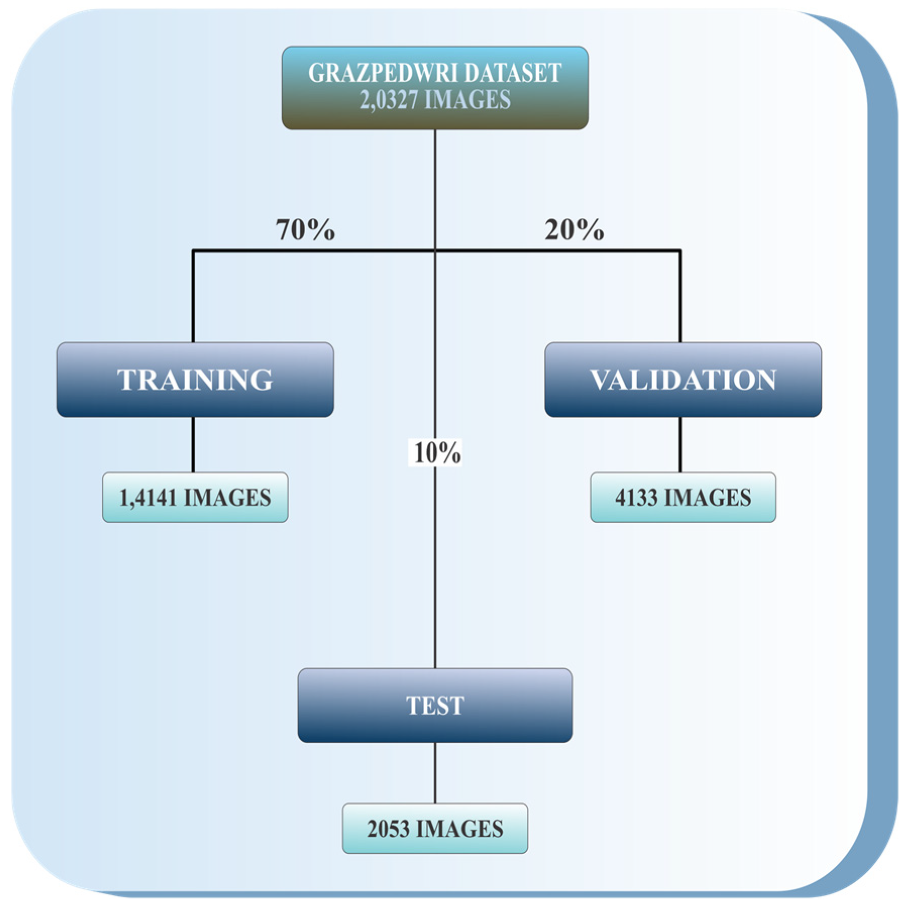
4.1. Dataset

In this experimental analysis, we utilized the GRAZPEDWRI-DX dataset [44], containing 20,327 wrist X-ray images. The images, stored in PNG format, were gathered from (6091) pediatric patients between 2008 to 2018 at the Pediatric Surgery Department of University Hospital Graz in Austria. The patients in this dataset are between 2 and 19 years old, with an average age of 10.9 years. It includes 2688 female patients, 3402 male patients, and one patient whose gender is not specified. Several pediatric radiology physicians used lines, bounding boxes, and polygons to mark the diagnosed conditions, such as fractures, periosteal reaction, and other pathologies in each image. For our study, we specifically selected the subset of images annotated with bounding boxes in the YOLO format, which includes eight different fractured classes of the dataset: Text, Fracture, Metal, Bone anomaly, Bone lesion, Periosteal reaction, Pronator sign, and Soft tissue. Following the data splitting and augmentation method, the dataset publisher did not provide some of the predefined splits, so we randomly distributed the dataset into three sections: training with 70% as 14,141 images, validation with 20% as 4133 images, and testing with 10% as 2053 images, as shown below in Figure 4.

• This dataset is general, containing 20,327 labelled and categorized images, and is ideal for developing and testing computer vision models.
• The dataset includes a wide variety of images capturing early bone development in children.
• Reviewing wrist development at this stage provides important insights for identifying, managing, and preventing abnormalities that might not be noticeable in adult wrists.

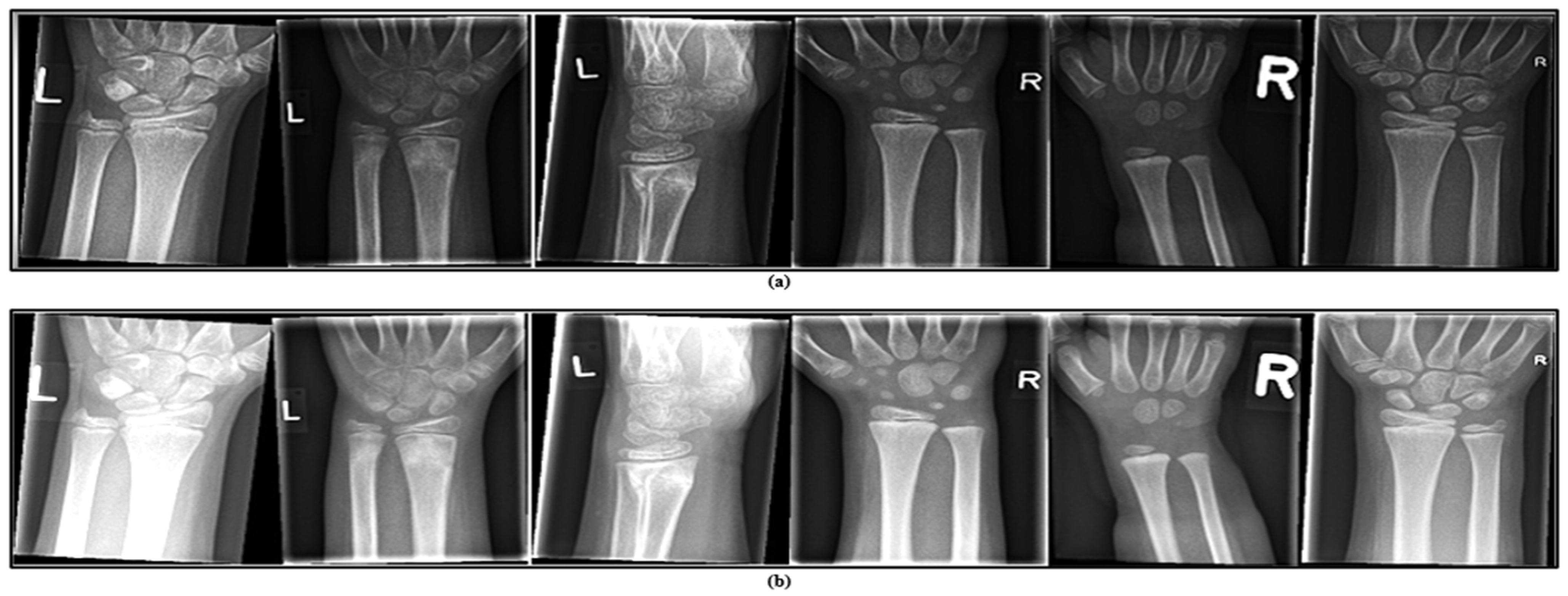
4.2. Data Preprocessing

We implemented several data preprocessing steps to ensure the dataset was well-structured and suitable for training the YOLO11 model. One of the key challenges we faced was the inconsistency in image sizes, which could affect the model’s capability to detect features exactly. To address this, we standardized all images by resizing them to 640 × 640 and 1024 × 1024 pixels. This resizing process not only ensured uniformity across the dataset but also optimized the input data for better model performance, improving both training efficiency and detection accuracy. We aimed to create a more robust and reliable training pipeline after applying the preprocessing techniques. Ultimately, this preprocessing strategy not only strengthens the training pipeline but also ensures the model’s strength and flexibility for many datasets, making it more scalable and well-organized for real-world deployment.

4.3. Data Augmentation

The limited brightness levels present in DX dataset X-ray images restrict the prediction accuracy of other X-ray images. The mode applies a data augmentation method to increase the training dataset, because this rectified model robustness. We applied the weighting function from the OpenCV library to manipulate brightness and contrast in the X-ray images for data augmentation. The data augmentation technique enabled the model to function effectively under different lighting scenarios and obtain training from multiple image types, thus extending the X-ray image database from an initial 14,141 to 28,282 instances as follows:

$$\mathrm{O}\mathrm{u}\mathrm{t}\mathrm{p}\mathrm{u}\mathrm{t}={\mathrm{I}\mathrm{n}\mathrm{p}\mathrm{u}\mathrm{t}}_1\times \mathrm{X}+{\mathrm{I}\mathrm{n}\mathrm{p}\mathrm{u}\mathrm{t}}_2\times \mathrm{Y}+\mathrm{Z}.$$

(31)

The equation is based on OpenCV’s add Weighted () function, which is commonly used for linear blending of two images (i.e., input₁ and input₂). Figure 5a corresponds to Input₁ and Figure 5b to Input₂; both are images of identical dimensions. In our implementation, they represent the same original image, reused within the equation to maintain a generalized and extensible formulation. X is the weight (scaling factor) for Input₁, used to control contrast. Y is the weight for Input₂. Since Input₂ is the same image and not intended to contribute to contrast adjustment, we set Y = 0 and Z is a scalar value added to all pixels to increase brightness. The weight refers to a specific value, a scaling factor that controls the contribution of each input image to the output as below:

The apparent brightness difference between Figure 5a,b may be influenced by several factors, including figure layout, rendering settings during export, or display-specific contrast scaling. Although Figure 5a may visually appear brighter at first glance, we confirm that Figure 5b corresponds to the image generated using the defined augmentation parameters: X = 1.5 (contrast scaling factor) and Z = 40 (brightness offset).

• Input1 (Figure 5a): Represents the original input images before augmentation.
• Input2 (Figure 5b): Represents the augmented images after applying the transformation.

4.4. Experimental Setup

We trained the YOLO11 model on the DX dataset. All models were resized to the target dimensions using a consistent scaling method for the sliced data. In this learning, we avoided overfitting during training by properly allotting the data and applying the dropout technique. First, we tested the pre-trained YOLO11 model from the Microsoft Common Objects in Context (MS COCO) val2017 dataset [68]. In model training, it is very important to choose the best hyperparameters for more effective model performance. In our experiments with YOLO variants, we used standard hyperparameters. The optimization algorithm we selected was the SGD [69], as the optimizer used to train the model needs fewer epochs for weight updates. Particularly, for the YOLO11m model with an input image size of 1024, the best performance is obtained at 27 epochs when trained with the SGD optimizer. Recently, Ultralytics released YOLO11 [70] on 30 September 2024 as their latest open-source model. In contrast, Ultralytics recommended YOLO11 training, and every model modified was trained for 100 epochs from scratch. We noted that the model’s mAP value started to stabilize between epochs 75 and 85. Following the Ultralytic recommendations, we set the optimizer’s weight decay to 5 × 10⁻⁴, momentum to 0.937, and the initial learning rate to 1 × 10⁻².

4.5. Model Training

We tested two different input image sizes, 640 px, and 1024 px, to see how they impact the model’s performance. The training on multiple NVIDIA TITAN RTX GPUs required an input image size of either 640 px or 1024 px with 24GB of GPU memory per card. GPUs with greater computing power and larger memory help significantly speed up the training process. The batch size was chosen based on user requirements and GPU memory limits; in our case, a batch size of 16 was used. The implementation is based on the v8.3.70 release of Ultralytics YOLO and utilizes the PyTorch framework. Python 3.12.8 was used for training with PyTorch 2.6.0 as the framework. We suggest using Python 3.12 or later and PyTorch 2.6 or newer for optimal model training.

5. Results and Discussion

In this section, we estimate the efficiency of the YOLO11 model with different attention modules. In the wrist fracture detection task, we checked the effect of different YOLO11 model versions (i.e., n, s, m, l) using 640 px and 1024 px input sizes to recognize their strengths and weaknesses. The best-performing variant is selected based on mAP at IoU 0.5 and recall at a 0.001 confidence threshold, focusing on fracture detection. For the model performance of the YOLO11, we introduce a novel method by incorporating three different attention modules, GAM, ResNet_GAM, and SE_BLOCK. to enrich the whole model performance of the YOLO11, precisely when the input image size is 1024 and the model size is medium. Finally, we used a confusion matrix to examine errors and ensure clinically reliable predictions for wrist bone displacement detection. To extend and validate our results, we showed an in-depth study of false positives and false negatives, optimizing the model’s sensitivity and specificity.

5.1. YOLO11 Results for All Classes

Below,

Table 1. Validation results of the YOLO11 model for each class on the GRAZPEDWRI-DX dataset using an input image size of 640.

Classes (640)	Images	Instances	Precision	Recall	mAPval 50	mAPval 50-95
Bone anomaly	30	35	0.59	0.171	0.241	0.111
Bone lesion	15	18	1.0	0.148	0.547	0.262
Fracture	2821	3789	0.81	0.902	0.93	0.55
Metal	133	155	0.88	0.955	0.967	0.799
Periosteal reaction	451	696	0.51	0.711	0.639	0.307
Pronator sign	110	110	0.62	0.745	0.714	0.389
Soft tissue	99	107	0.43	0.327	0.306	0.149
Text	4123	4790	0.96	0.984	0.992	0.752

and

Table 2. Validation results of the YOLO11 model for each class on the GRAZPEDWRI-DX dataset using an input image size of 1024.

Classes (1024)	Images	Instances	Precision	Recall	mAPval 50	mAPval 50-95
Bone anomaly	30	35	1.0	0.113	0.205	0.084
Bone lesion	15	18	1.0	0.257	0.535	0.274
Fracture	2821	3789	0.87	0.894	0.938	0.559
Metal	133	155	0.85	0.942	0.966	0.763
Periosteal reaction	451	696	0.44	0.76	0.652	0.327
Pronator sign	110	110	0.70	0.726	0.737	0.413
Soft tissue	99	107	0.61	0.175	0.304	0.143
Text	4123	4790	0.95	0.987	0.992	0.758

present the complete analysis of all-classes validation using input image sizes of 640 px and 1024 px to estimate, based on precision, recall, mAP50, and mAP50-95 for eight different classes. Fracture, Metal, and Text consistently gain high precision and recall, with mAP50 values above 0.9 at both image sizes, indicating that they are the easiest to detect. In contrast, bone anomaly and soft tissue are the most challenging classes, showing low recall and mAP50-95 scores of 0.111 at 640 px and 0.084 at 1024 px for bone anomaly. Increasing the image size to 1024 px enhances precision for bone anomaly from 0.59 to 1.0 and soft tissue from 0.43 to 0.61, but reduces recall. Bone anomaly drops from 0.171 to 0.113, indicating a trade-off where the model becomes more conservative but misses more actual detections. However, Fracture, Metal, and Text maintain high mAP values above 0.5 in mAP50-95, showing strong performance across different IoU thresholds. Furthermore, the higher input resolution slightly improves the detection of certain fine-grained structures, such as pronator signs and periosteal reactions, as reflected in their enlarged precision and marginal improvement in mAP50-95. However, the results also specify diminishing returns in recall for some rare classes, signifying that increasing resolution alone does not always guarantee better generalization. These findings highlight the importance of carefully selecting input resolution dependent on the target pathology, as higher resolution may improve localization confidence.

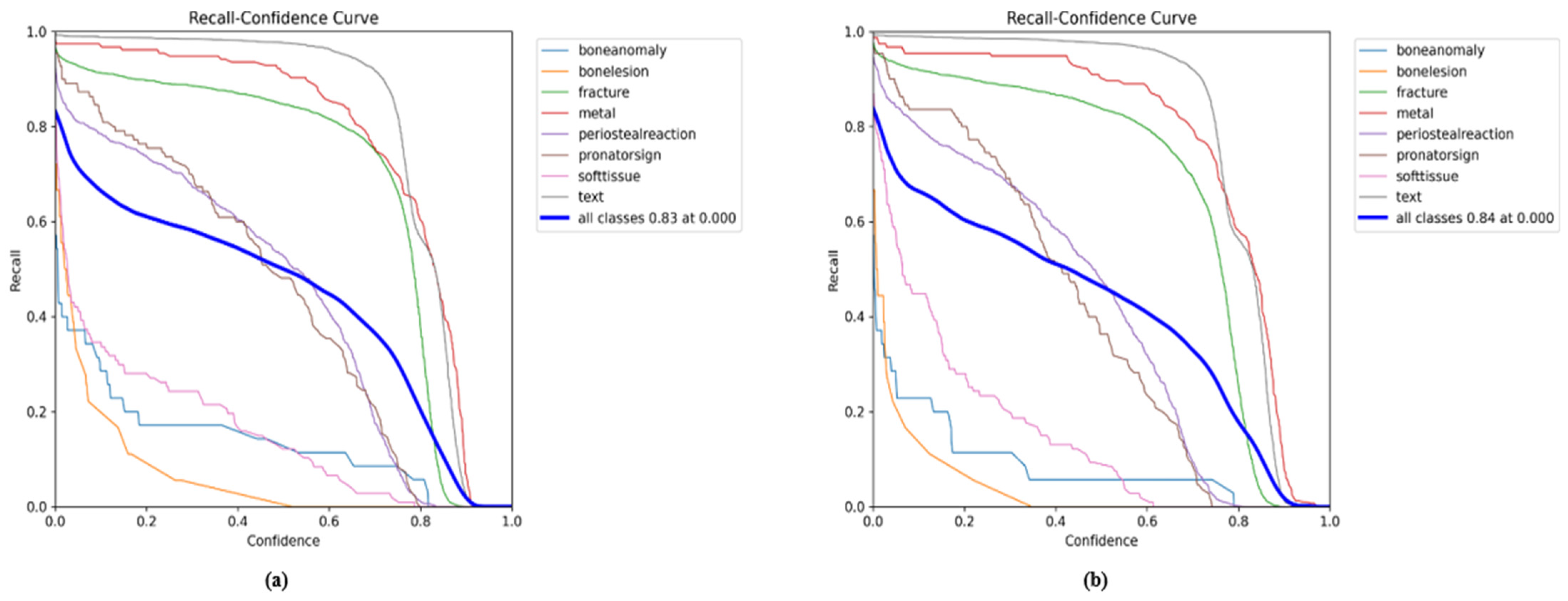
5.2. Comparison Results of YOLO11n with GAM and ResNet_GAM

Table 3. Experimental results for wrist fracture detection using the YOLO11n model, comparing performance with two different attention modules: GAM and ResNet_GAM.

Model-11n	Input Size	Prams (M)	Inference (ms)	GFLOP’s	Precision	Recall	mAPval 50	mAPval 50-95
YOLO11	640	2.583	1.1	6.3	0.680	0.553	0.585	0.380
GAM	640	3.548	0.8	14.4	0.706	0.549	0.603	0.382
RES_GAM	640	5.393	0.9	15.2	0.723	0.554	0.611	0.376
YOLO11	1024	2.583	1.3	6.3	0.703	0.565	0.588	0.381
GAM	1024	3.547	2.2	11.4	0.799	0.554	0.617	0.378
RES_GAM	1024	5.399	2.2	15.2	0.717	0.602	0.624	0.380

displays the performance of the YOLO11n, GAM, and ResNet_GAM at 640 px and 1024 px, evaluating mAP50, Precision, Recall, GFLOPs, and inference time. The ResNet_GAM model succeeds in the maximum detection accuracy, with a mean average precision of mAP@50 of 62.4% for 1024 px images, which is 2.13% higher than the 61.1% for 640 px images. However, inference time rises from 0.9 ms to 2.2 ms due to the larger model size. The GAM module also elevates detection performance, increasing mAP@50 by 2.32%, from 0.603 at 640 px to 0.617 at 1024 px. The YOLO11 model has the lowest performance at both image sizes, with a mAP@50 of 0.585 at 640 px and 0.588 at 1024 px, compared to GAM and ResNet_GAM. Meanwhile, GAM achieves its highest precision of 0.799 at 1024 px and ResNet_GAM delivers a better balance, achieving 0.717 Precision and a maximum Recall of 0.602 at 1024 px, reducing missed fractures. In contrast, YOLO11 has the lowest mAP@50, Precision, and Recall, making it the least accurate model. Overall, ResNet_GAM demonstrates outstanding performance by effectively balancing Precision and Recall, ensuring better detection accuracy and minimizing missed fractures. In addition, the GFLOP comparison reveals that, while ResNet_GAM has a higher computational cost (1.9 at 1024 px), its performance justifies the added complexity in high-accuracy scenarios. GAM is computationally lighter than ResNet_GAM.

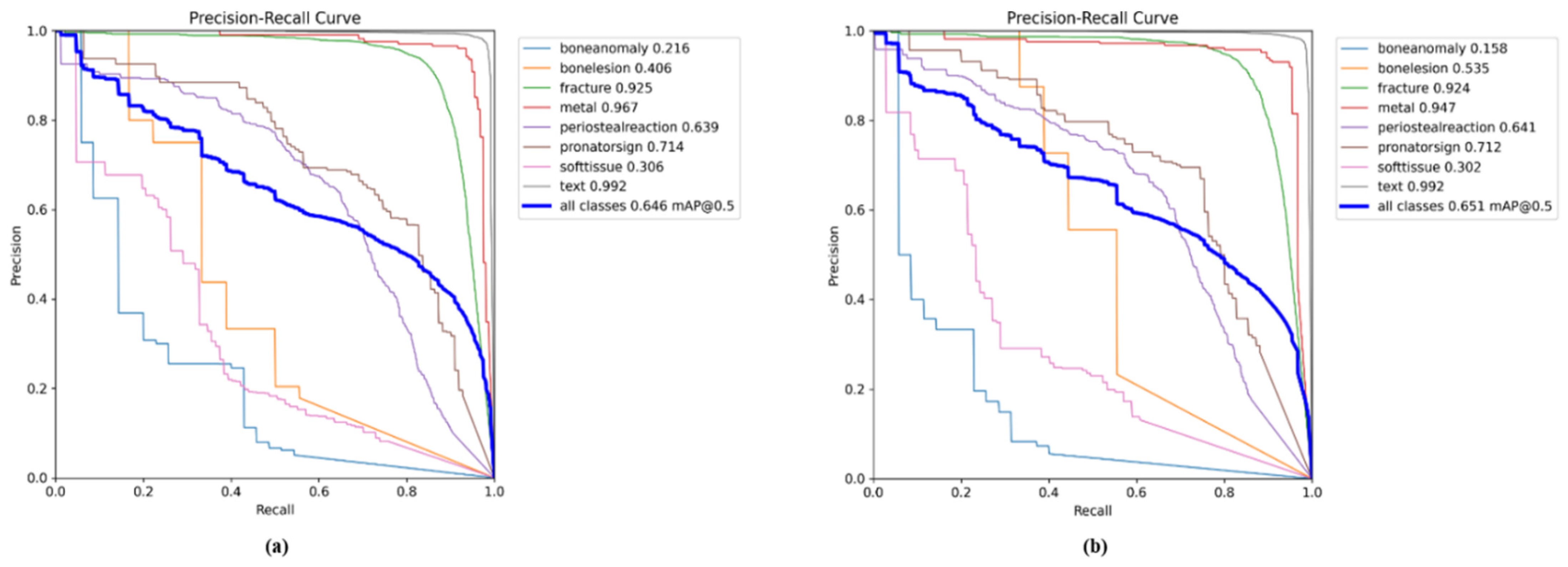
5.3. Comparison Results of YOLO11s with GAM and ResNet_GAM

Table 4. Experimental results for wrist fracture detection using the YOLO11s model, comparing performance with two different attention modules: GAM and ResNet_GAM.

Model-11m	Input Size	Prams (M)	Inference (ms)	GFLOP’s	Precision	Recall	mAPval 50	mAPval 50-95
YOLO11	640	20.93	2.3	67.7	0.639	0.599	0.626	0.415
GAM	640	35.288	4.0	163.5	0.731	0.601	0.618	0.383
RES_GAM	640	50.631	5.7	212.6	0.623	0.639	0.637	0.394
YOLO11	1024	20.036	5.4	67.7	0.639	0.610	0.638	0.417
GAM	1024	35.288	12.5	163.5	0.573	0.632	0.636	0.396
RES_GAM	1024	50.631	9.8	212.6	0.633	0.590	0.641	0.397

shows the results of the YOLO11s baseline model, along with GAM and ResNet_GAM. The YOLO11 “s” variant performs well in mAP@50 compared to the “n” variant, especially when using ResNet_GAM and GAM at both 640 px and 1024 px image sizes. The version ‘‘s’’ displays outstanding performance in detecting fractures by excelling in both mAP@50 and mAP@50-95. Notably, the ResNet_GAM delivered the best performance with the “s” version, achieving a mAP@50 of 0.627 at 640 px and 0.643 at 1024 px. It also displayed the highest mAP@50-95 of 0.408 at 1024 px, leading both YOLO11 and GAM. However, YOLO11 and GAM show small enrichment at 0.33% and 1.46%, respectively, at 1024 px, higher resolution has minimal impact on precise localization. ResNet_GAM also leads in Precision 0.692 at 640 px, 0.653 at 1024 px, and Recall 0.615 at 1024 px, detecting fractures more correctly while minimizing missed cases. Overall, the “s” version of ResNet_GAM and GAM exceed as compared to the previous version.

5.4. Comparison Results of YOLO11m with GAM and ResNet_GAM

Table 5. Experimental results for wrist fracture detection using the YOLO11m model, comparing performance with two different attention modules: GAM and ResNet_GAM.

Model-11s	Input Size	Prams (M)	Inference (ms)	GFLOP’s	Precision	Recall	mAPval 50	mAPval 50-95
YOLO11	640	9.416	2.2	21.3	0.665	0.551	0.606	0.392
GAM	640	14.101	1.8	45.1	0.649	0.633	0.617	0.385
RES_GAM	640	21.479	2.1	60.2	0.692	0.603	0.627	0.394
YOLO11	1024	9.416	2.8	21.2	0.546	0.574	0.608	0.398
GAM	1024	14.101	4.4	45.1	0.666	0.598	0.626	0.392
RES_GAM	1024	21.479	5.7	60.2	0.653	0.615	0.643	0.408

provides the wrist fracture detection output of the YOLO11m model, highlighting its effectiveness compared to the “n” and “s” versions. This model variant outperforms the smaller versions due to its significantly higher parameter count of 50.631M and GFLOPs 212.6, which require extra computation but the accuracy is enhanced. ResNet_GAM, while achieving the best results, is also the slowest, with inference time increasing from 5.7 ms to 9.8 ms due to its larger model size. In contrast, YOLO11 remains the fastest at 2.3 ms at 640 px, and 5.4 ms at 1024 px, due to its lightweight architecture. ResNet_GAM achieves the best detection performance in all the versions. In the below table, we showed that the highest mAP@50 of 0.637 at 640 px, 0.641 at 1024 px, and localization accuracy mAP@50-95 of 0.394 at 640 px, 0.397 at 1024 px. It also obtained the highest recall 0.632 at 1024 px, detecting more true fractures. Meanwhile, GAM has the greatest precision, attaining 0.731 at 640 px, with a slight mAP@50 improvement from 0.618 at 640 px to 0.636 at 1024 px, indicating minor detection gains at higher resolution. Overall, ResNet_GAM provides the best balance between precision, recall, and mAP scores, producing it the most effective model for wrist fracture detection. GAM enhances precision, while YOLO11 remains the fastest but least accurate option.

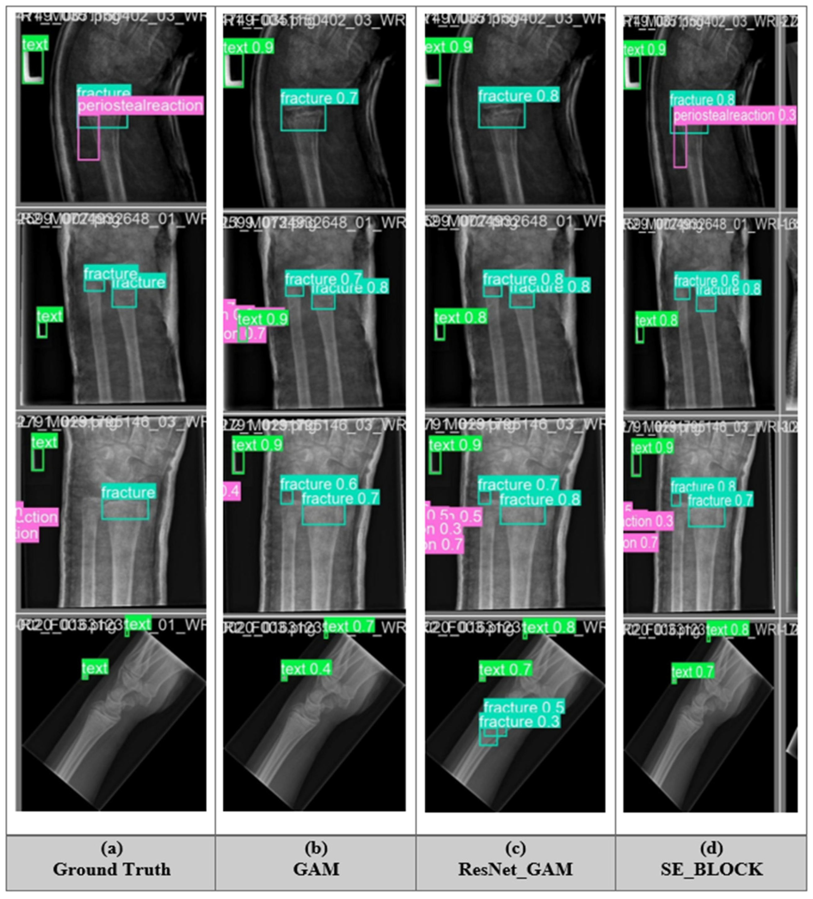
5.5. Fracture Detection of All Model

The fracture detection performance of different YOLO11 models was improved with attention mechanisms. The first column represents the Ground Truth (GT), showing the actual fractures and text annotations, while the following three columns display predictions from different attention-refined YOLO11 models: GAM (i.e., Global Attention Mechanism), ResNet_GAM (i.e., Residual Global Attention Mechanism), and SE_BLOCK (i.e., Squeeze-and-Excitation Block), displayed below in Figure 6. The bounding boxes indicate detected fractures (i.e., cyan), text regions (i.e., green), and Periosteal reactions (i.e., magenta), each with confidence scores. From the comparison, it is evident that the models vary in their ability to detect fractures accurately. The SE_BLOCK model appears to detect more fractures with higher confidence scores, suggesting that it captures fine details effectively. GAM and ResNet_GAM models offer balanced detections, identifying fractures with reasonable confidence but sometimes missing smaller or less distinct ones. The GT box serves as a benchmark, highlighting the actual fracture locations, against which the model predictions can be evaluated. The image demonstrates the role of attention mechanisms in enhancing the diagnostic accuracy of YOLO11 with ResNet_GAM for medical imaging applications. The ResNet_GAM model, functioning as a CAD tool, assists radiologists in detecting fractures, improving the efficiency and reliability of diagnoses. This graphical analysis additionally confirms that attention-based modules not only help in locating fractures but also decrease false positives in non-fracture regions. The better-quality localization and confidence scores, particularly with SE_BLOCK, highlight the effectiveness of channel-wise recalibration. Such improvements are vital in clinical scenarios, where accurate interpretation of subtle signs in X-rays is essential for early diagnosis and timely treatment planning. Moreover, integrating attention into lightweight detection frameworks ensures faster inference with high sensitivity, which is helpful for point-of-care and real-time analysis.

5.6. GAM and ResNet_GAM Model Performance on Different Image Size

The figures below illustrate the detailed performance of the GAM model across eight classes, comparing results for two input image resolutions: 640 px and 1024 px. Figure 7 presents the precision-recall (PR) curves for each of the eight target classes. The thick dark blue curve indicates the overall mAP@0.5, while the colored lines represent the performance for each individual class. A slight improvement in mAP is observed from 0.634 at 640 px to 0.636 at 1024, when using higher resolution images. Figure 8 highlights the performance of the ResNet_GAM model, which outperforms the standalone GAM model at both resolutions. The mAP@0.5 for ResNet_GAM increases from 0.637 at 640 px to 0.643 at 1024 px. This improvement is attributed to the ResNet backbone providing robust base features, which are further refined by the GAM module, resulting in enhanced precision-recall curves. Notably, the classes fracture, metal, and text exhibit high precision and recall across both models, indicating strong and consistent performance in these categories.

Figure 9 illustrates the recall versus confidence curves for both models. The x-axis represents the confidence threshold ranging from 0 to 1, while the y-axis shows the recall (true positive rate). The thick blue line indicates the macro-average recall across all classes at varying confidence levels. The value displayed in the bottom-right corner (e.g., “all classes: 0.83 at 0.000”) represents the maximum recall achieved at a zero-confidence threshold. For the ResNet_GAM model, recall remains strong at lower confidence thresholds (0.0 to 0.3), achieving an average class recall of 0.83. In comparison, the GAM model demonstrates a slightly better overall recall curve, with a macro-average recall of 0.84. Figure 10 presented the F1 score and confidence threshold curves for the GAM and ResNet_GAM models. The x-axis represents the confidence threshold used to accept predictions, while the y-axis shows the F1 score, which is the harmonic mean of precision and recall, providing a balanced measure of model performance. The ResNet_GAM model achieves a maximum F1 score of 0.62 at a confidence threshold of 0.127, whereas the GAM model reaches a maximum F1 score of 0.61 at a threshold of 0.218. Comparatively, the GAM model demonstrates a good precision-recall balance but is more sensitive to changes in confidence threshold. On the other hand, ResNet_GAM not only achieves a slightly higher F1 score but also shows greater robustness at lower confidence levels, making it more stable and reliable in early prediction stages.

5.7. Ablation Study

This study further examines the effect of integrating the SE_BLOCK module into the YOLO11 model at input resolutions of 640 and 1024. The results indicate that SE_BLOCK significantly increases the model’s complexity, with the number of parameters nearly doubling from 25.286M in the original YOLO11 to 49.318M at 640 px and 49.319M at 1024 px. Similarly, the computational cost of GFLOPs rises substantially from 60.0 to 172.3 at 640 px and from 86.6 to 172.3 at 1024 px. The inference time also increases from 3.4 ms to 4.7 ms at 640 px and from 8.2 ms to 11.5 ms at 1024 px, highlighting the balance between model complexity and computational efficiency. Regarding detection performance, the introduction of SE_BLOCK improves precision across both resolutions, increasing from 0.637 to 0.700 at 640 px and from 0.680 to 0.705 at 1024 px, indicating a reduction in false positives. However, recall shows a slight fluctuation, increasing from 0.606 to 0.614 at 640 px inputs while slightly decreasing from 0.613 to 0.605 at 1024 px inputs. At an IoU threshold of mAPval50, the model’s performance improves, increasing from 0.635 to 0.646 at an input size of 640 px and from 0.646 to 0.651 at 1024 px, represented in Figure 11. This demonstrates that the SE_BLOCK helps make detections more reliable. However, under stricter evaluation conditions mAPval50-95, which measure accuracy across a broader range of IoU thresholds, the performance slightly drops. The mAPval50-95 value drops from 0.423 to 0.408 at 640 px and from 0.425 to 0.410 at 1024 px, as displayed in

Table 6. YOLO large model performance using our SE_BLOCK method with 640 px and 1024 px image sizes.

SE_BLOCK	Input Size	Prams (M)	Inference (ms)	GFLOP’s	Precision	Recall	mAPval 50	mAPval 50-95
YOLO11	640	25.286	3.4	60.0	0.637	0.606	0.635	0.423
SE_BLOCK	640	49.318	4.7	172.3	0.700	0.614	0.646	0.408
YOLO11	1024	25.286	8.2	86.6	0.680	0.613	0.646	0.425
SE_BLOCK	1024	49.319	11.5	172.3	0.705	0.605	0.651	0.410

. This suggests that, while SE_BLOCK improves detection confidence, its effectiveness reduces when tested under more difficult conditions. Additionally, other variations of the SE_BLOCK amplified YOLO11 model, namely SE_BLOCK (i.e., n, s, m), were not included in this study as they did not yield satisfactory results for this dataset. These versions failed to reach competitive performance, either due to excessive computational overhead or suboptimal feature enhancement, making them unsuitable for this specific rail flaw detection task. The findings suggest that, while SE_BLOCK improves precision and leads to moderate IoU mAP scores, this comes as the result of increased model size and computational burden scores. Furthermore, its limited uplift in recall and strict IoU performance highlights a trade-off between detection confidence and the ability to identify a higher number of true positives.

5.8. Evaluate the Model Training and Confusion Matrix

In Figure 12 describe the training and validation loss curves, which consistently decrease throughout the training process. This indicates effective learning and the absence of overfitting. The dotted orange line represents a smoothed version of the loss curve for better visualization. Additionally, various evaluation metrics are displayed to assess the model’s performance during training. The metrics/precision(B) refers to the proportion of correctly predicted positive detections among all predictions, while metrics/recall(B) indicates the proportion of true positives that were correctly identified. Figure 13 presents the Normalized Confusion Matrix for the YOLOv11m-GAM model. It provides a visual summary of the model’s performance in a multi-class classification task, including a background class.

• Comparison Results for Proposed Method (

  Table 7. Comparison of the precision and mAPval 50 proposed wrist fracture detection model with existing state-of-the-art (SOTA) methods using the GRAZPEDWRI-DX dataset.

  Model	Precision	mAPval 50
  YOLOv5n [71]	0.77	0.590
  YOLOv6n [71]	0.50	0.510
  YOLOv7n [71]	0.59	0.500
  YOLOv8n [71]	0.73	0.590
  YOLOv6s [71]	0.51	0.620
  YOLOv6m [71]	0.59	0.64
  YOLOv8m [71]	0.60	0.60
  YOLOv6L [71]	0.60	0.640
  Ours YOLO-11n	0.79	0.610
  Ours YOLO-11s	0.69	0.627
  Ours YOLO-11m	0.63	0.641
  Ours YOLO-11L	0.70	0.651

  ,

  Table 8. Comparison of the mAPval 50 and mAPval 50-95 proposed wrist fracture detection model with existing state-of-the-art (SOTA) methods using the GRAZPEDWRI-DX dataset.

  Model	mAPval 50	mAPval 50-95
  Image Size-640
  YOLOv6n [72]	0.605	0.379
  YOLOv7n [72]	0.612	0.392
  YOLOv8n [72]	0.629	0.404
  YOLOv6s [72]	0.637	0.406
  Image Size-1024
  YOLOv8m [72]	0.608	0.391
  YOLOv6L [72]	0.631	0.402
  YOLOv8m [72]	0.635	0.411
  YOLOv6L [72]	0.638	0.415
  Ours Image Size-640
  YOLO-11n	0.611	0.376
  YOLO-11s	0.627	0.394
  YOLO-11m	0.637	0.394
  YOLO-11L	0.646	0.408
  Ours Image Size-1024
  YOLO-11n	0.624	0.380
  YOLO-11s	0.643	0.408
  YOLO-11m	0.641	0.397
  YOLO-11L	0.651	0.410

  and

  Table 9. Comparison of the Precision, Recall, mAPval 50 and mAPval 50-95 proposed wrist fracture detection model with existing state-of-the-art (SOTA) methods using the GRAZPEDWRI-DX dataset.

  Model	Precision	Recall	mAPval 50	mAPval 50-95
  YOLOv7 [73]	0.774	0.536	0.544	0.326
  YOLOv8 [74]	0.778	0.546	0.591	0.372
  Ours YOLO-11	0.799	0.554	0.617	0.378

  )

5.9. Application

This study introduces a Bone Fracture Detection System displayed in Figure 14 that combines deep learning with an easy-to-use graphical interface and detects the number of target categories in the picture. Users can simply upload an image through the interface, where it is automatically resizes to 400 × 400 pixels for consistent processing with a single click on the “Detect Disease” button, and the model scans the image, highlighting fractures The result is then displayed back to the user with clear visual markers. Built using CustomTkinter, Tkinter, and PIL, the interface is designed for simplicity and efficiency, making it accessible even to those with minimal technical expertise, and also helps surgeons accurately locate and classify bone pathology, reducing the likelihood of incorrect analysis and providing more useful information for surgery. This system aims to support medical professionals by providing a quick, AI-powered second opinion, ultimately enhancing diagnostic accuracy and speeding up the fracture detection process. The GitHub link accesses the web-based application. Furthermore, the system’s modular design allows for easy combination with hospital management systems and electronic medical records (EMRs), providing seamless data accessibility for healthcare professionals. Future improvements include increasing the dataset to develop model simplification and integrating additional fractured detection abilities. In addition, the platform is being enhanced to support real-time diagnosis for emergency room settings where time-critical decisions are essential. Further refinements will focus on including explainable AI (XAI) techniques to provide transparency behind predictions, helping radiologists understand and trust the model’s outputs. Mobile application deployment is also under consideration to extend its reach in low-resource or remote environments.

6. Conclusions

In this paper, we presented an enhanced YOLO11_AM model for the detection of wrist injury, integrating GAM, ResNet_GAM, and SE_BLOCK. Among these, ResNet_GAM achieved the best performance, with mAP50 values of 63.7% at 640 px and 64.3% at 1024 px, effectively balancing precision and recall. While SE_BLOCK improved precision, it significantly increased computational complexity, making real-time deployment challenging. Additionally, higher resolution 1024 px) enhanced precision but did not always improve recall, indicating the need for further optimizations in detecting bone anomalies and soft tissue injuries. Future research should focus on optimizing model efficiency for real-time applications through techniques like quantization and lightweight attention mechanisms. AI diagnostic systems would improve radiologists’ efficiency and diagnostic accuracy. Hybrid deep learning approaches, such as combining CNNs with Vision Transformers, could further refine detection accuracy. Furthermore, incorporating Explainable AI techniques would increase model interpretability, increasing trust and adoption in clinical settings.

References

1. Abbas, W.; Adnan, S.M.; Javid, M.A.; Majeed, F.; Ahsan, T.; Hassan, S.S. Lower leg bone fracture detection and classification using faster RCNN for X-ray images. In Proceedings of the 2020 IEEE 23rd International Multitopic Conference (INMIC), Bahawalpur, Pakistan, 5–7 November 2020; IEEE: Piscataway, NJ, USA, 2020; pp. 1–6. [Google Scholar]
2. International Osteoporosis Foundation. Broken Bones, Broken Lives: A Roadmap to Solve the Fragility Fracture Crisis in Europe; International Osteoporosis Foundation: Nyon, Switzerland, 2018. [Google Scholar]
3. Hedström, E.M.; Svensson, O.; Bergström, U.; Michno, P. Epidemiology of fractures in children and adolescents: Increased incidence over the past decade: A population-based study from northern Sweden. Acta Orthop. 2010, 81, 148–153. [Google Scholar] [CrossRef] [PubMed]
4. Randsborg, P.H.; Gulbrandsen, P.; Benth, J.Š.; Sivertsen, E.A.; Hammer, O.L.; Fuglesang, H.F.; Årøen, A. Fractures in children: Epidemiology and activity-specific fracture rates. JBJS 2013, 95, e42. [Google Scholar] [CrossRef]
5. Landin, L.A. Epidemiology of children’s fractures. J. Pediatr. Orthop. B 1997, 6, 79–83. [Google Scholar] [CrossRef]
6. Cheng, J.C.; Shen, W.Y. Limb fracture pattern in different pediatric age groups: A study of 3350 children. J. Orthop. Trauma 1993, 7, 15–22. [Google Scholar] [CrossRef]
7. McCollough, C.H.; Bushberg, J.T.; Fletcher, J.G.; Eckel, L.J. Answers to common questions about the use and safety of CT scans. Mayo Clin. Proc. 2015, 90, 1380–1392. [Google Scholar] [CrossRef]
8. Burr David, B. Introduction–Bone turnover and fracture risk. J. Musculoskelet. Neuronal. Interact. 2003, 3, 408–409. [Google Scholar]
9. Yadav, D.P.; Rathor, S. Bone fracture detection and classification using deep learning approach. In Proceedings of the 2020 International Conference on Power Electronics & IoT Applications in Renewable Energy and its Control (PARC), Mathura, India, 28–29 February 2020; IEEE: Piscataway, NJ, USA, 2020; pp. 282–285. [Google Scholar]
10. Anu, T.C.; Raman, R. Detection of bone fracture using image processing methods. Int. J. Comput. Appl. 2015, 975, 8887. [Google Scholar]
11. Hallas, P.; Ellingsen, T. Errors in fracture diagnoses in the emergency department–characteristics of patients and diurnal variation. BMC Emerg. Med. 2006, 6, 4. [Google Scholar] [CrossRef]
12. Guly, H.R. Diagnostic errors in an accident and emergency department. Emerg. Med. J. 2001, 18, 263–269. [Google Scholar] [CrossRef]
13. Mounts, J.; Clingenpeel, J.; McGuire, E.; Byers, E.; Kireeva, Y. Most frequently missed fractures in the emergency department. Clin. Pediatr. 2011, 50, 183–186. [Google Scholar] [CrossRef]
14. Erhan, E.R.; Kara, P.H.; Oyar, O.; Unluer, E.E. Overlooked extremity fractures in the emergency department. Ulus Travma Acil Cerrahi Derg 2013, 19, 25–28. [Google Scholar]
15. Juhl, M.; Moller-Madsen, B.; Jensen, J. Missed injuries in an orthopedic department. Injury 1990, 21, 110–112. [Google Scholar] [CrossRef] [PubMed]
16. Burki, T.K. The shortfall of consultant clinical radiologists in the UK. Lancet Oncol. 2018, 19, 518. [Google Scholar] [CrossRef] [PubMed]
17. Rimmer, A. Radiologist shortage leaves patient care at risk, warns royal college. BMJ Br. Med. J. 2017, 359, 4683. [Google Scholar] [CrossRef]
18. Body, J.J.; Acklin, Y.P.; Gunther, O.; Hechmati, G.; Pereira, J.; Maniadakis, N.; Terpos, E.; Finek, J.; von Moos, R.; Talbot, S.; et al. Pathologic fracture and healthcare resource utilisation: A retrospective study in eight European countries. J. Bone Oncol. 2016, 5, 185–193. [Google Scholar] [CrossRef]
19. Rosman, D.A.; Nshizirungu, J.J.; Rudakemwa, E.; Moshi, C.; de Dieu Tuyisenge, J.; Uwimana, E.; Kalisa, L. Imaging in the land of 1000 hills: Rwanda radiology country report. J. Glob. Radiol. 2015, 1, 5. [Google Scholar] [CrossRef]
20. Smith-Bindman, R.; Kwan, M.L.; Marlow, E.C.; Theis, M.K.; Bolch, W.; Cheng, S.Y.; Bowles, E.J.; Duncan, J.R.; Greenlee, R.T.; Kushi, L.H.; et al. Trends in use of medicasl imaging in US health care systems and Ontario, Canada, 2000–2016. JAMA 2019, 322, 843–856. [Google Scholar] [CrossRef]
21. Chhem, R.K. Radiation protection in medical imaging: A never-ending story? Eur. J. Radiol. 2010, 76, 1–2. [Google Scholar] [CrossRef]
22. Neubauer, J.; Benndorf, M.; Reidelbach, C.; Krauß, T.; Lampert, F.; Zajonc, H.; Kotter, E.; Langer, M.; Fiebich, M.; Goerke, S.M. Comparison of diagnostic accuracy of radiation dose-equivalent radiography, multidetector computed tomography, and cone beam computed tomography for fractures of adult cadaveric wrists. PLoS ONE 2016, 11, e0164859. [Google Scholar] [CrossRef]
23. Tanzi, L.; Vezzetti, E.; Moreno, R.; Aprato, A.; Audisio, A.; Massè, A. Hierarchical fracture classification of proximal femur X-ray images using a multistage Deep Learning approach. Eur. J. Radiol. 2020, 133, 109373. [Google Scholar] [CrossRef]
24. Choi, J.W.; Cho, Y.J.; Lee, S.; Lee, J.; Lee, S.; Choi, Y.H.; Cheon, J.E.; Ha, J.Y. Using a dual-input convolutional neural network for automated detection of pediatric supracondylar fracture on conventional radiography. Investig. Radiol. 2020, 55, 101–110. [Google Scholar] [CrossRef] [PubMed]
25. Chung, S.W.; Han, S.S.; Lee, J.W.; Oh, K.S.; Kim, N.R.; Yoon, J.P.; Kim, J.Y.; Moon, S.H.; Kwon, J.; Lee, H.J.; et al. Automated detection and classification of the proximal humerus fracture by using a deep learning algorithm. Acta Orthop. 2018, 89, 468–473. [Google Scholar] [CrossRef] [PubMed]
26. Gan, K.; Xu, D.; Lin, Y.; Shen, Y.; Zhang, T.; Hu, K.; Zhou, K.; Bi, M.; Pan, L.; Wu, W.; et al. Artificial intelligence detection of distal radius fractures: A comparison between the convolutional neural network and professional assessments. Acta Orthop. 2019, 90, 394–400. [Google Scholar] [CrossRef] [PubMed]
27. Kim, D.H.; MacKinnon, T. Artificial intelligence in fracture detection: Transfer learning from deep convolutional neural networks. Clin. Radiol. 2018, 73, 439–445. [Google Scholar] [CrossRef]
28. Lindsey, R.; Daluiski, A.; Chopra, S.; Lachapelle, A.; Mozer, M.; Sicular, S.; Hanel, D.; Gardner, M.; Gupta, A.; Hotchkiss, R.; et al. Deep neural network improves fracture detection by clinicians. Proc. Natl. Acad. Sci. USA 2018, 115, 11591–11596. [Google Scholar] [CrossRef]
29. Urakawa, T.; Tanaka, Y.; Goto, S.; Matsuzawa, H.; Watanabe, K.; Endo, N. Detecting intertrochanteric hip fractures with orthopedist-level accuracy using a deep convolutional neural network. Skelet. Radiol. 2019, 48, 239–244. [Google Scholar] [CrossRef]
30. Yahalomi, E.; Chernofsky, M.; Werman, M. Detection of distal radius fractures trained by a small set of X-ray images and Faster R-CNN. In Intelligent Computing: Proceedings of the 2019 Computing Conference; Springer International Publishing: Berlin/Heidelberg, Germany, 2019; Volume 1, pp. 971–981. [Google Scholar]
31. Redmon, J.; Divvala, S.; Girshick, R.; Farhadi, A. You only look once: Unified, real-time object detection. In Proceedings of the IEEE Conference on Computer Vision and Pattern Recognition, Las Vegas, NV, USA, 27–30 June 2016; pp. 779–788. [Google Scholar]
32. Ju, R.Y.; Chen, C.C.; Chiang, J.S.; Lin, Y.S.; Chen, W.H. Resolution enhancement processing on low-quality images using a swim transformer based on interval interval-dense connection strategy. Multimed. Tools Appl. 2024, 83, 14839–14855. [Google Scholar] [CrossRef]
33. Hržić, F.; Tschauner, S.; Sorantin, E.; Štajduhar, I. Fracture recognition in pediatric wrist radiographs: An object detection approach. Mathematics 2022, 10, 2939. [Google Scholar] [CrossRef]
34. Samothai, P.; Sanguansat, P.; Kheaksong, A.; Srisomboon, K.; Lee, W. The evaluation of bone fracture detection of yolo series. In Proceedings of the 2022 37th International Technical Conference on Circuits/Systems, Computers and Communications (ITC-CSCC), Phuket, Thailand, 5–8 July 2022; IEEE: Piscataway, NJ, USA, 2022; pp. 1054–1057. [Google Scholar]
35. Huang, Z.; Wang, X.; Huang, L.; Huang, C.; Wei, Y.; Liu, W. Ccnet: Criss-cross attention for semantic segmentation. In Proceedings of the IEEE/CVF International Conference on Computer Vision, Seoul, Republic of Korea, 27 October–2 November 2019; pp. 603–612. [Google Scholar]
36. Wu, S.; Wang, J.; Liu, L.; Chen, D.; Lu, H.; Xu, C.; Hao, R.; Li, Z.; Wang, Q. Enhanced YOLOv5 Object Detection Algorithm for Accurate Detection of Adult Rhynchophorus ferruginous. Insects 2023, 14, 698. [Google Scholar] [CrossRef]
37. Das, S.; Bhattachya, D.; Biswas, T. Detection of Bone Fractures Along with Other Abnormalities in Wrist X-Ray Images Using Enhanced-Yolo11. Available online: https://ouci.dntb.gov.ua/en/works/4gVVAd17/ (accessed on 1 April 2025).
38. Nagy, E.; Janisch, M.; Hržić, F.; Sorantin, E.; Tschauner, S. A pediatric wrist trauma X-ray dataset (GRAZPEDWRI-DX) for machine learning. Sci. Data 2022, 9, 222. [Google Scholar] [CrossRef]
39. Woo, S.; Park, J.; Lee, J.Y.; Kweon, I.S. Cbam: Convolutional block attention module. In Proceedings of the European Conference on Computer Vision (ECCV), Munich, Germany, 8–14 September 2018; pp. 3–19. [Google Scholar]
40. He, K.; Zhang, X.; Ren, S.; Sun, J. Deep residual learning for image recognition. In Proceedings of the IEEE Conference on Computer Vision and Pattern Recognition, Las Vegas, NV, USA, 27–30 June 2016; pp. 770–778. [Google Scholar]
41. Hardalaç, F.; Uysal, F.; Peker, O.; Çiçeklidağ, M.; Tolunay, T.; Tokgöz, N.; Kutbay, U.; Demirciler, B.; Mert, F. Fracture detection in wrist X-ray images using deep learning-based object detection models. Sensors 2022, 22, 1285. [Google Scholar] [CrossRef] [PubMed]
42. Liu, X.; Faes, L.; Kale, A.U.; Wagner, S.K.; Fu, D.J.; Bruynseels, A.; Mahendiran, T.; Moraes, G.; Shamdas, M.; Kern, C.; et al. A comparison of deep learning performance against health-care professionals in detecting diseases from medical imaging: A systematic review and meta-analysis. Lancet Digit. Health 2019, 1, e271–e297. [Google Scholar] [CrossRef]
43. Xu, Y.; Hosny, A.; Zeleznik, R.; Parmar, C.; Coroller, T.; Franco, I.; Mak, R.H.; Aerts, H.J. Deep learning predicts lung cancer treatment response from serial medical imaging. Clin. Cancer Res. 2019, 25, 3266–3275. [Google Scholar] [CrossRef]
44. Zhou, S.K.; Greenspan, H.; Davatzikos, C.; Duncan, J.S.; Van Ginneken, B.; Madabhushi, A.; Prince, J.L.; Rueckert, D.; Summers, R.M. A review of deep learning in medical imaging: Imaging traits, technology trends, case studies with progress highlights, and future promises. Proc. IEEE 2021, 109, 820–838. [Google Scholar] [CrossRef]
45. Rahimzadeh, M.; Attar, A.; Sakhaei, S.M. A fully automated deep learning-based network for detecting COVID-19 from a new and large lung CT scan dataset. Biomed. Signal Process. Control. 2021, 68, 102588. [Google Scholar] [CrossRef] [PubMed]
46. Kalmet, P.H.; Sanduleanu, S.; Primakov, S.; Wu, G.; Jochems, A.; Refaee, T.; Ibrahim, A.; Hulst, L.V.; Lambin, P.; Poeze, M. Deep learning in fracture detection: A narrative review. Acta Orthop. 2020, 91, 215–220. [Google Scholar] [CrossRef] [PubMed]
47. Hsieh, C.I.; Zheng, K.; Lin, C.; Mei, L.; Lu, L.; Li, W.; Chen, F.P.; Wang, Y.; Zhou, X.; Wang, F.; et al. Automated bone mineral density prediction and fracture risk assessment using plain radiographs via deep learning. Nat. Commun. 2021, 12, 472. [Google Scholar] [CrossRef]
48. Kuznetsova, A.; Maleva, T.; Soloviev, V. Detecting apples in orchards using YOLOv3 and YOLOv5 in general and close-up images. In Advances in Neural Networks–ISNN 2020: 17th International Symposium on Neural Networks, ISNN 2020, Cairo, Egypt, 4–6 December 2020; Proceedings 17; Springer International Publishing: Berlin/Heidelberg, Germany, 2020; pp. 233–243. [Google Scholar]
49. Burkow, J.; Holste, G.; Otjen, J.; Perez, F.; Junewick, J.; Alessio, A. Avalanche decision schemes to improve pediatric rib fracture detection. In Medical Imaging 2022: Computer-Aided Diagnosis; SPIE: Washington, WA, USA, 2022; Volume 12033, pp. 611–618. [Google Scholar]
50. Tsai, H.C.; Qu, Y.Y.; Lin, C.H.; Lu, N.H.; Liu, K.Y.; Wang, J.F. Automatic rib fracture detection and localization from frontal and oblique chest X-rays. In Proceedings of the 2022 10th International Conference on Orange Technology (ICOT), Shanghai, China, 10–11 November 2022; pp. 1–4. [Google Scholar]
51. Warin, K.; Limprasert, W.; Suebnukarn, S.; Paipongna, T.; Jantana, P.; Vicharueang, S. Maxillofacial fracture detection and classification in computed tomography images using convolutional neural network-based models. Sci. Rep. 2023, 13, 3434. [Google Scholar] [CrossRef]
52. Yuan, G.; Liu, G.; Wu, X.; Jiang, R. An improved yolov5 for skull fracture detection. In International Symposium on Intelligence Computation and Applications; Springer Nature: Singapore, 2021; pp. 175–188. [Google Scholar]
53. Mushtaq, M.; Akram, M.U.; Alghamdi, N.S.; Fatima, J.; Masood, R.F. Localization and edge-based segmentation of lumbar spine vertebrae to identify the deformities using deep learning models. Sensors 2022, 22, 1547. [Google Scholar] [CrossRef]
54. Meza, G.; Ganta, D.; Gonzalez Torres, S. Deep Learning Approach for Arm Fracture Detection Based on an Improved YOLOv8 Algorithm. Algorithms 2024, 17, 471. [Google Scholar] [CrossRef]
55. Ren, S.; He, K.; Girshick, R.; Sun, J. Faster r-cnn: Towards real-time object detection with region proposal networks. Adv. Neural Inf. Process. Syst. 2015, 28, 91–99. [Google Scholar] [CrossRef] [PubMed]
56. Ma, Y.; Luo, Y. Bone fracture detection through the two-stage system of Crack-Sensitive Convolutional Neural Network. Inf. Med. Unlocked 2020, 22, 100452. [Google Scholar] [CrossRef]
57. Su, Z.; Adam, A.; Nasrudin, M.F.; Ayob, M.; Punganan, G. Skeletal fracture detection with deep learning: A comprehensive review. Diagnostics 2023, 13, 3245. [Google Scholar] [CrossRef]
58. Nguyen, H.T.; Tran, T.B.; Tran, T.T. Fracture Detection in Bone: An Approach with Versions of YOLOv4. SN Comput. Sci. 2024, 5, 765. [Google Scholar] [CrossRef]
59. Sha, G.; Wu, J.; Yu, B. Detection of spinal fracture lesions based on improved Yolov2. In Proceedings of the 2020 IEEE International Conference on Artificial Intelligence and Computer Applications (ICAICA), Dalian, China, 27–29 June 2020; pp. 235–238. [Google Scholar]
60. Fan, Q.; Brown, L.; Smith, J. A closer look at Faster R-CNN for vehicle detection. In Proceedings of the 2016 IEEE Intelligent Vehicles Symposium (IV), Gothenburg, Sweden, 19–22 June 2016; IEEE: Piscataway, NJ, USA, 2016; pp. 124–129. [Google Scholar]
61. Thian, Y.L.; Li, Y.; Jagmohan, P.; Sia, D.; Chan, V.E.Y.; Tan, R.T. Convolutional neural networks for automated fracture detection and localization on wrist radiographs. Radiol. Artif. Intell. 2019, 1, e180001. [Google Scholar] [CrossRef] [PubMed]
62. Hu, J.; Shen, L.; Sun, G. Squeeze-and-excitation networks. In Proceedings of the IEEE Conference on Computer Vision and Pattern Recognition, Salt Lake City, UT, USA, 18–23 June 2018; pp. 7132–7141. [Google Scholar]
63. Chen, Y.; Kalantidis, Y.; Li, J.; Yan, S.; Feng, J. A^ 2-nets: Double attention networks. Adv. Neural Inf. Process. Syst. 2018, 31. [Google Scholar]
64. Liu, Y.; Shao, Z.; Hoffmann, N. Global attention mechanism: Retain information to enhance channel-spacial Interaction. arXiv 2021, arXiv:2112.05561. [Google Scholar]
65. Wang, Q.; Wu, B.; Zhu, P.; Li, P.; Zuo, W.; Hu, Q. ECA-Net: Efficient channel attention for deep convolutional neural networks. In Proceedings of the IEEE/CVF Conference on Computer Vision and Pattern Recognition, Seattle, WA, USA, 13–19 June 2020; pp. 11534–11542. [Google Scholar]
66. Zhang, Q.L.; Yang, Y.B. Sa-net: Shuffle attention for deep convolutional neural networks. In Proceedings of the ICASSP 2021–2021 IEEE International Conference on Acoustics, Speech and Signal Processing (ICASSP), Toronto, ON, Canada, 6–11 June 2021; IEEE: Piscataway, NJ, USA, 2021; pp. 2235–2239. [Google Scholar]
67. Lin, T.Y.; Maire, M.; Belongie, S.; Hays, J.; Perona, P.; Ramanan, D.; Dollár, P.; Zitnick, C.L. Microsoft coco: Common objects in context. In Proceedings of the Computer Vision–ECCV 2014: 13th European Conference, Zurich, Switzerland, 6–12 September 2014; Springer International Publishing: Berlin/Heidelberg, Germany, 2014; pp. 740–755. [Google Scholar]
68. Ruder, S. An overview of gradient descent optimization algorithms. arXiv 2016, arXiv:1609.04747. [Google Scholar]
69. Jegham, N.; Koh, C.Y.; Abdelatti, M.; Hendawi, A. YOLO Evolution: A Comprehensive Benchmark and Architectural Review of YOLOv12, YOLO11, and Their Previous Versions. Yolo11, and Their Previous Versions. arXiv 2025, arXiv:2411.00201. [Google Scholar]
70. Ke, H.; Li, H.; Wang, B.; Tang, Q.; Lee, Y.H.; Yang, C.F. Integrations of LabelImg, You Only Look Once (YOLO), and Open-Source Computer Vision Library (OpenCV) for Chicken Open Mouth Detection. Sens. Mater. 2024, 36, 4903. [Google Scholar] [CrossRef]
71. Ahmed, A.; Imran, A.S.; Manaf, A.; Kastrati, Z.; Daudpota, S.M. Enhancing wrist abnormality detection with yolo: Analysis of state-of-the-art single-stage detection models. Biomed. Signal Process. Control. 2024, 93, 106144. [Google Scholar] [CrossRef]
72. Ju, R.Y.; Cai, W. Fracture detection in pediatric wrist trauma X-ray images using YOLOv8 algorithm. Sci. Rep. 2023, 13, 20077. [Google Scholar] [CrossRef] [PubMed]
73. Till, T.; Tschauner, S.; Singer, G.; Lichtenegger, K.; Till, H. Development and optimization of AI algorithms for wrist fracture detection in children using a freely available dataset. Front. Pediatr. 2023, 11, 1291804. [Google Scholar] [CrossRef] [PubMed]
74. Erzen, E.M.; BÜtÜn, E.; Al-Antari, M.A.; Saleh, R.A.; Addo, D. Artificial Intelligence Computer-Aided Diagnosis to automatically predict the Pediatric Wrist Trauma using Medical X-ray Images. In Proceedings of the 2023 7th International Symposium on Innovative Approaches in Smart Technologies (ISAS), Istanbul, Turkey, 23–25 November 2023; pp. 1–7. [Google Scholar]
Figure 1. YOLO11 Residual Block (Res_Block) integrated with the Convolutional Block Attention Module (ResNet_GAM) architecture.
Mathematics 13 01419 g001
Figure 2. ResNet_GAM Architecture.
Mathematics 13 01419 g002
Figure 3. Squeeze-and-Excitation (SE_BLOCK).
Mathematics 13 01419 g003
Figure 4. Data Splitting.
Mathematics 13 01419 g004
Figure 5. Representation of pediatric wrist X-rays with data augmentation presented through two sets of images: (a) shows the image after adding modifications and (b) shows the original image.
Mathematics 13 01419 g005
Figure 6. Examples of results of different YOLO11 models applied to pediatric wrist fracture detection and Ground-Truth: (a) Manually labelled data; (b) GAM (c) ResNet_GAM (d) SE_BLOCK.
Mathematics 13 01419 g006
Figure 7. Precision vs. Recall Results of the GAM (a) 640 px (b) 1024 px.
Mathematics 13 01419 g007
Figure 8. Precision vs. Recall Results of ResNet_ GAM (a) 640 px (b) 1024 px.
Mathematics 13 01419 g008
Figure 9. Recall vs. Precision Results of (a) ResNet_GAM (b) GAM.
Mathematics 13 01419 g009
Figure 10. F1-Confidence Curve of (a) GAM (b) ResNet_GAM.
Mathematics 13 01419 g010
Figure 11. Precision vs. Recall results of the SE_BLOCK (a) 640 px (b) 1024 px.
Mathematics 13 01419 g011
Figure 12. Graphical Representation of Training and Validation Metrics.
Mathematics 13 01419 g012
Figure 13. Confusion Matrix (YOLO11m GAM).
Mathematics 13 01419 g013
Figure 14. Fracture Detection with YOLO11 Web-based Interface.
Mathematics 13 01419 g014