A Lightweight Model of Learning Common Features in Different Domains for Classification Tasks

Abstract

The increasing size of recent deep neural networks, particularly when applied to learning across multiple domains, limits their deployment in resource-constrained environments. To address this issue, this study proposes a lightweight neural architecture with a parallel structure of convolutional layers to enable efficient and scalable multi-domain learning. The proposed network includes an individual feature extractor for domain-specific features and a common feature extractor for the shared features. This design minimizes redundancy and significantly reduces the number of parameters while preserving classification performance. To evaluate the proposed method, experiments were conducted using four image classification datasets: MNIST, FMNIST, CIFAR10, and SVHN. These experiments focused on classification settings where each image contained a single dominant object without relying on large pretrained models. The proposed model achieved high accuracy while significantly reducing the number of parameters. It required only 3.9 M parameters for learning across the four datasets, compared to 33.6 M for VGG16. The model achieved an accuracy of 98.87% on MNIST and 85.83% on SVHN, outperforming other lightweight models, including MobileNet v2 and EfficientNet v2b0, and was comparable to ResNet50. These findings indicate that the proposed architecture has the potential to support multi-domain learning while minimizing model complexity. This approach may be beneficial for applications in resource-constrained environments.

1. Introduction

In recent years, computer systems have progressed exponentially, enabling them to perform complex tasks within a few seconds. The growing availability of large-scale datasets and increasing computational power have enabled deep learning to perform various tasks in computer vision, including image classification and object detection. However, deep-learning models can be costly and resource-intensive, requiring large amounts of data and computing power for specific tasks. In scenarios where data availability is limited or computing power is expensive, a transfer learning model may be a suitable solution [1]. The network can learn the general features of various classes from large-scale data and incorporate the learned weights into the model to initialize the training and classification using an entirely new dataset. Transfer learning solves a novel problem by using a pretrained neural network and adapting it to a new dataset through the transfer of the features of the source domain. An essential component of transfer learning is the use of a pre-trained model, which is a backbone network trained on a large dataset, such as ImageNet [2] or MS COCO [3]. In terms of computer vision, ImageNet and MS COCO are challenging, high-quality datasets primarily used to build state-of-the-art neural networks. ImageNet, released in 2009, comprises 1000 classes and 14 M images and is widely used for object detection, pose estimation, and image classification. MS COCO is a representative image-captioning dataset that comprises 2 M images and 80 classes.

When using a small-scale dataset, the pretrained model must be fine-tuned to fit the smaller dataset and achieve high performance. Transfer learning models are commonly used for domain adaptation [4,5], few-shot learning [6,7], and zero-shot learning [8], among others. However, a model that fine-tunes a pretrained model has a large capacity and requires more computational expenses for model inference [9]. Therefore, such a model is unsuitable for devices with deficient resources, such as mobile devices and services, which require frequent deployment.

A lightweight network structure addresses these challenges by efficiently minimizing the model capacity; therefore, several studies have applied deep learning to resource-constrained environments [10,11,12,13,14]. Lightweight models are examined from two perspectives: (1) lightweight network design and (2) model compression. Lightweight network design focuses on constructing compact architectures that reduce computational and memory costs. Representative examples include MobileNet [15], EfficientNet [16], and ConvNeXt-Tiny [17], which leverage depthwise convolution, pointwise convolution, and efficient channel-wise operations to achieve parameter-efficient designs. Conversely, model compression reduces the model capacity and inference cost by removing redundant parameters or operations while maintaining performance. Representative model compression techniques include pruning [18,19,20], quantization [21,22,23], and knowledge distillation [24,25,26], which typically require large-scale datasets for pretraining. When new data that are not represented in the pretrained model are encountered, generating effective lightweight models from the pretrained model becomes challenging.

To overcome these limitations, we propose a mechanism that enables the direct learning of common features from multiple datasets without requiring large pretrained models, thus enabling efficient multidomain learning to handle a new dataset that was not used for the pretrained model. This approach reduces the dependency on large-scale datasets and simplifies the training process, making it more flexible and scalable for various applications.

This lightweight model architecture not only reduces the number of parameters but also maintains high accuracy by simultaneously learning common and domain-specific features. This design facilitates the efficient deployment of resource-constrained devices without compromising performance. Unlike traditional model-compression algorithms or network redesigns, our approach eliminates the need for complex post-training operations and offers an intuitive structure with broad usability and scalability.

The proposed model comprises an individual feature extractor (IndvFE) for learning the individual features of each dataset and a common feature extractor (ComFE) for learning the common features of the entire dataset. To validate the proposed method, we conducted experiments to classify images using datasets from four different domains. Specifically, we selected MNIST, Fashion-MNIST (FMNIST), CIFAR10, and SVHN, which are popular public datasets used for image classification. For implementation, we used various combinations of datasets and evaluated the three models used in our methods. The results showed that the model with a ComFE can reduce the number of parameters and maintain better performance than the model without the proposed method.

The remainder of this paper is organized as follows: Section 2 analyzes the related work. Section 3 introduces the dataset used in this study and the proposed network architecture, including its structure and learning cycle. Section 4 presents the experimental setup and results. Section 5 and Section 6 discuss the insights and potential research directions, respectively.

2. Related Work

Deep-learning model compression encompasses two main areas of study: (a) methods for reducing the layers or operations in a model’s network, yielding lightweight network models, and (b) model compression algorithms.

2.1. Lightweight Network Models

In computer vision, lightweight models have become increasingly essential, particularly for deployment in devices with limited computational resources, such as mobile phones and embedded systems. These models aim to reduce computational complexity while maintaining a high performance. Iandola et al. [12] proposed SqueezeNet, which uses a 1 × 1 convolution instead of a 3 × 3 convolution to reduce the number of network parameters. Howard et al. [13] proposed MobileNet for mobile and embedded vision applications to ensure efficient operation while maintaining the performance. Its structure is based on a streamlined architecture in which depthwise separable convolutions are first applied in channel units to build lightweight deep neural networks. Subsequently, a pointwise convolution is applied to the output. Zhang et al. [14] proposed ShuffleNet, a convolutional neural network fundamentally based on MobileNet, aimed at maximizing efficiency by performing only essential channel operations and applying pointwise group convolution. Wan and Yao [27] introduced LMFRNet, which is based on the novel concept of convolutional layers that integrate the structures of inception [28] and residual blocks [29]. Li et al. [30] presented EfficientFormer, a lightweight model of a vision transformer (ViT) that reduces the complexity of the transformer blocks and substitutes them with convolutional block layers. Mehta and Rastegari [31] proposed MobileViT, which combines convolutions with ViT layers while ignoring positional encoding. Sharma et al. [32] introduced a method for narrowing channels to reduce the number of parameters in a network architecture.

Zoph et al. [33] introduced an automated method for identifying the optimal network architecture for a given dataset. This method, termed neural architecture search, uses reinforcement learning to identify the best convolutional layer architecture. Tan et al. [34] proposed MnasNet, which explicitly considers the model latency for mobile devices. Han et al. [35] proposed GhostNet, which reduces the number of required convolution operations by generating feature vectors, termed “ghost” features, through cost-effective linear operations. Wu et al. [36] developed FBNet, representing another attempt to build a lightweight network model through the search for an optimal architecture. This method involves initially training a stochastic network. Subsequently, the optimal architectures are sampled from the trained distributions. Tan and Le [37] proposed EfficientNet, which searches for the optimal network by scaling up the network size, starting from a base architecture.

Although these approaches have proven effective in various scenarios, our study explores a complementary direction by constructing a compact model for multiple small-scale datasets using shared features.

2.2. Model Compression Algorithms

Unlike network redesign methods, model-compression algorithms, such as pruning, quantization, and knowledge distillation, adjust networks after a model is trained. Pruning removes the relationships between nodes that have a low impact on the network results. Molchanov et al. [18,20] and Tung and Mori [38] emphasized the importance of pruning in maintaining a method based on Taylor expansion. Furthermore, Tung and Mori [38] improved the compression rate by combining network pruning and weight quantization in parallel.

Quantization further enhances the inference performance by converting the model weights from floating points to integers. Zhu et al. [23] introduced a trained ternary quantization to divide the weights into three parts. Cai et al. [21] proposed ZeroQ, a zero-shot quantization method that avoids retraining the original or validation dataset. Wang et al. [22] developed a joint search method for model architecture, pruning, and quantization (APQ) policies.

Unlike pruning and quantization, knowledge distillation involves training a small model using a pretrained model [26]. This process enables the transfer of knowledge from a large, unwieldy model or set of models to a single smaller model that can be practically applied to real-world constraints. This approach is sometimes referred to as teacher–student learning. To improve retrieval performance and reduce computational cost, Zhai et al. [39] introduced a technique that minimizes the distribution of hashing codes of the teacher and student models, distilling knowledge from a complex teacher latent layer into a student model that contains significantly more supervised information than image labels. Mullapudi et al. [25] proposed low-cost video semantic segmentation for a target video stream through model distillation. Yin et al. introduced deep inversion, a method that enables data-free knowledge transfer [24].

Model-compression techniques generally focus on post-training optimization. The proposed approach emphasizes efficiency through architectural design from the beginning of training.

3. Materials and Methods

3.1. Network Architecture

In multi-domain learning, training independent models for each domain leads to a linear increase in the number of parameters as the number of datasets increases. In addition, each model may suffer from a limited number of training samples within its domain. In contrast, using a single feature extractor requires an increased model capacity to learn features across multiple domains [40]. The increase in model capacity is largely attributed to the requirement for a single feature extractor to learn one shared set of parameters that can represent multiple domains simultaneously. In this study, we assumed that the load of the shared feature extractor could be reduced if a small network undertakes in part the task of extracting domain-specific features, because the common extractor no longer needs to encode multiple domain-specific variations within a single shared parameterization; instead, these variations are handled by the domain-specific branch, enabling the common extractor to focus on representations that are reusable across domains. This motivates a two-extractor alternative in which feature extraction is decomposed into a shared ComFE and dataset-specific individual feature extractors (IndvFEs), placed in parallel to reduce parameter redundancy while preserving domain-dependent representations.

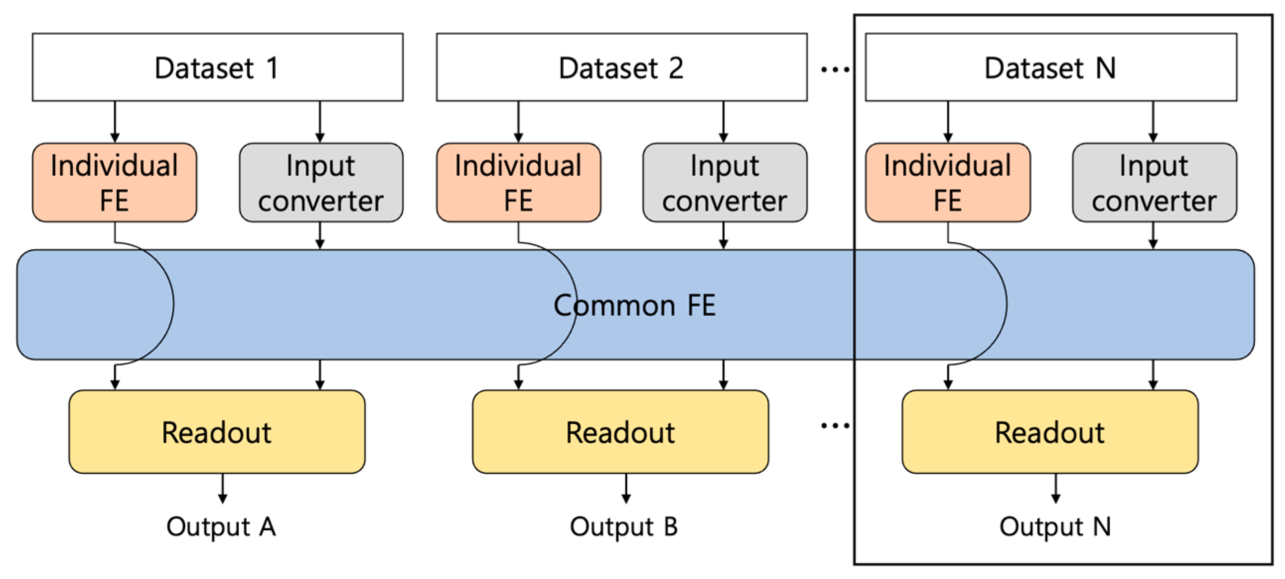
The overall architecture of the proposed model comprises a ComFE, multiple IndvFEs, an input converter, and a readout module, as shown in Figure 1. This architecture is designed for multi-domain learning, where multiple datasets from different domains are jointly exploited. Each dataset is associated with its own IndvFE, which learns domain-specific representations, whereas the shared ComFE learns domain-invariant features from all datasets. The IndvFEs acquire the original images from each dataset, whereas the ComFE branch is preceded by an input converter that maps input images of different sizes to a common feature-map size required by the ComFE. The features produced by the IndvFE and ComFE branches are then passed to the readout module, which concatenates the outputs from the two branches and generates the final classification output.

This study considers two architectural variants: a Base model (ComFE-Base) and a lightweight Tiny model (ComFE-Tiny). Both models adhere to the same top-level design but differ in the internal structure of their feature-extraction modules. The Base model is designed to provide a stable reference architecture and investigate whether the ComFE can exploit shared features across domains to reduce the number of parameters while improving recognition performance. However, the use of multiple convolutional blocks in the Base model results in a relatively high number of floating-point operations (FLOPs). To alleviate this computational burden, the Tiny model replaces the standard convolutions with depthwise convolutions, substantially reducing the FLOPs. Formally, we define the proposed deep learning model as a function $\mathsf{\Phi }(X;x,\theta ,\lambda )$, where $X$ is an input, $\theta$ denotes trainable parameters, and $\lambda$ specifies the structural configuration of the network modules. Note that the parameter set $\theta$ depends on $\lambda$. The Base and Tiny variants are then given by $\mathsf{\Phi }(X;x,\theta ,{\lambda }_{Base})$ and $\mathsf{\Phi }(X;x,\theta ,{\lambda }_{Tiny})$, respectively.

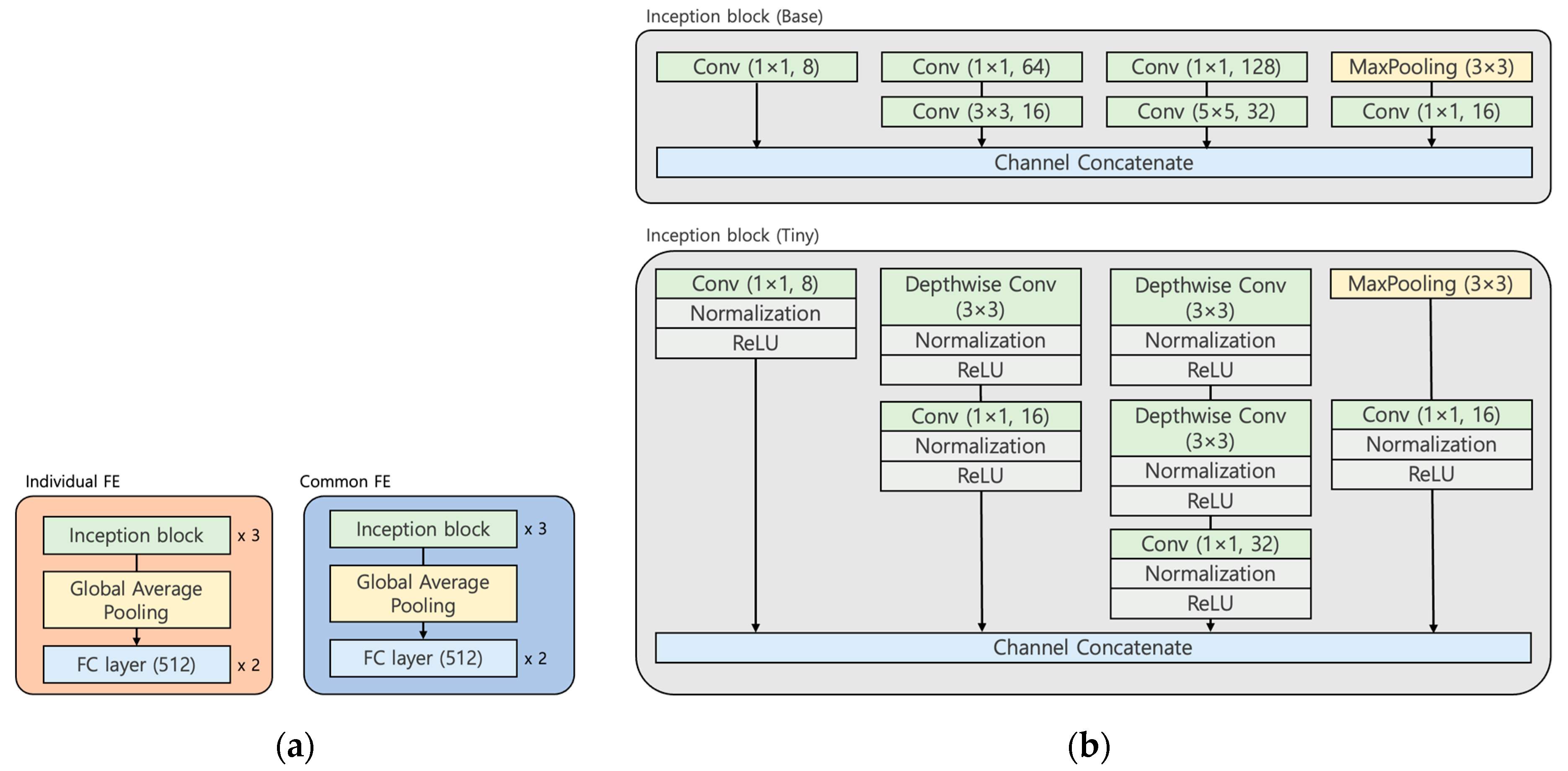
Both the IndvFEs and ComFE serve as feature-extraction modules in the proposed architecture and follow the same high-level design. As illustrated in Figure 2a, each module processes its input through a sequence of inception blocks [28], followed by global average pooling and a fully connected layer that produces a 512-dimensional embedding. The IndvFEs directly receive the original images from their corresponding datasets, whereas the ComFE operates on the feature maps produced by the input converter.

The feature-extraction backbone in both the IndvFEs and ComFE comprises stacked inception modules, whose detailed structure is illustrated in Figure 2b. Each inception module comprises multiple parallel branches designed to capture spatial information at various scales. In the Base model, one branch applies a 1 × 1 convolution to preserve fine-grained local information, whereas two additional branches apply 3 × 3 and 5 × 5 convolutions to extract broader contextual patterns. A max-pooling branch followed by a 1 × 1 convolution is also included to project the pooled features to a controlled channel dimensionality. The outputs of all branches are concatenated along the channel dimension to merge the multi-scale features.

In the Tiny model, the same multi-branch structure is preserved; however, the standard convolutions in each branch are replaced with a depthwise convolutional block, which comprises a depthwise convolution followed by normalization and ReLU (rectifiled linear unit) activation. In addition, a pointwise convolutional block—comprising a 1 × 1 convolution followed by normalization and ReLU activation—is used in place of each pointwise convolution. The pointwise convolutional blocks are placed at the end of each branch to mix the channel-wise features after depthwise spatial filtering.

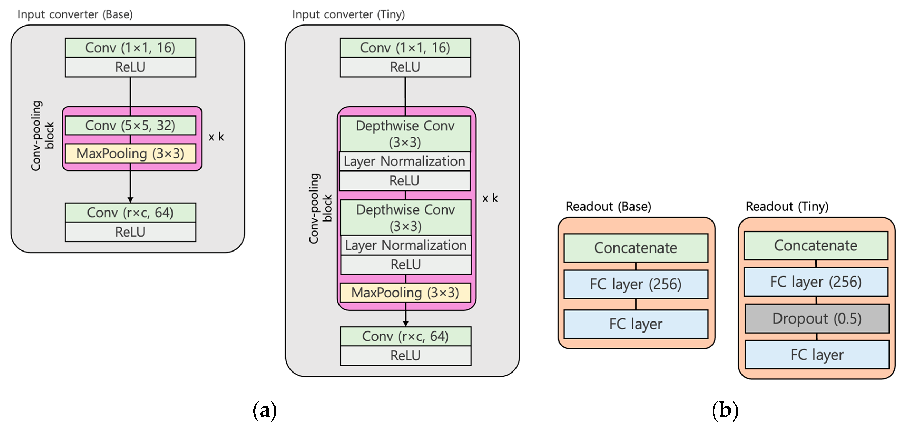
Figure 3 illustrates the input converter and readout module, highlighting how they interface with the ComFE for feature alignment and final classification. Specifically, the input converter reduces the spatial resolution using repeated convolution–pooling modules followed by an adaptive r × c convolution. The number $k$ of convolution-pooling modules and the kernel size ($r, c$) of the adaptive convolution are defined as follows:

$$k=max\left\{k|⌊{\displaystyle \frac{H}{2^k}}⌋>H_t, ⌊{\displaystyle \frac{W}{2^k}}⌋>W_t\right\},$$

(1)

$$\begin{gathered} \left(r,c\right)=\left(H_k-H_t+1, W_k-W_t+1\right), \\ {(H}_k,W_k)=\left(⌊{\displaystyle \frac{H}{2^k}}⌋, ⌊{\displaystyle \frac{W}{2^k}}⌋\right), \end{gathered}$$

(2)

where $H$ and $W$ are the height and width of the input image, respectively, and $H_t$ and $W_t$ are the target resolutions required by the ComFE. The input converter reduces the size of the features through repeated convolution–pooling blocks, instead of applying a direct resizing operation, because downsampling via a resize function may discard important visual information.

The readout module internally concatenates the feature representations produced by the IndvFE and ComFE branches and maps the combined representation to the final classification output. This module is implemented as a compact head comprising two dense layers. The first dense layer projects the concatenated features to a lower-dimensional space with 256 units, and the second dense layer outputs class-wise prediction scores.

To explicitly relate the proposed ComFE–IndvFE structure in Figure 1, Figure 2 and Figure 3 to the network size, we express the total number of parameters in each module. Let $D$ denote the number of domains. The proposed model comprises domain-specific front-end feature extractors (FE blocks), a shared ComFE, domain-specific IndvFEs, and domain-dependent readout heads. The total parameter count of the proposed model ($N_{proposed}$) is given by

$$N_{proposed}=N_{ComFE}+{\sum }_{d=1}^D\left(N_{IC}^{\left(d\right)}-N_{IndvFE}^{\left(d\right)}+N_{Out}\left(K_d\right)\right),$$

(3)

where $N_{IC}^{\left(d\right)}$ denotes the number of parameters of the front-end input converter preceding the ComFE for domain $d$, $N_{ComFE}$ denotes the number of parameters of the ComFE, $P_{IndvFE}^{\left(d\right)}$ denotes the number of parameters of the IndvFE for domain $d$, and $N_{Out}\left(K_d\right)$ denotes the number of parameters of the domain-dependent readout head with $K_d$ classes.

The readout head receives the concatenation of the outputs of the ComFE and IndvFE. Let $F_{com}$ and $F_{ind}$ denote the output dimensions of the ComFE and IndvFE, respectively, and $F_r$ denote the hidden dimension of the readout layer. The parameter count of the readout head ($N_{Out}$) is then expressed as

$$N_{Out}\left(K_d\right)=\left(\left(F_{com}+F_{ind}\right)·F_r-F_r\right)+\left(F_r·K_d+K_d\right).$$

(4)

3.2. Dataset

Table 1. Metadata of the four image datasets: number of classes, image size, and sample counts for training and testing.

Metadata	Dataset
	MNIST	FMNIST	CIFAR10	SVHN
Class	10	10	10	10
Image size	28 × 28 × 1	28 × 28 × 1	32 × 32 × 3	32 × 32 × 3
Number of training data	60,000	60,000	50,000	76,257
Number of test data	10,000	10,000	10,000	26,032

lists the datasets used in the experiments. These datasets were selected because they represent widely used public benchmarks for image classification with a unified 10-class setting. They also exhibit diverse visual characteristics across domains, such as grayscale versus color images and varying background complexity. This diversity naturally introduces domain variations, making the datasets suitable for evaluating the proposed multi-domain learning framework, which aims to capture both shared and domain-specific representations. The MNIST dataset [41] comprises 60,000 small square 28 × 28 pixel grayscale images of handwritten single digits between 0 and 9. The FMNIST [42] dataset consists of 60,000 training images and 10,000 test images from ten classes of clothing examples, such as shoes, shirts, and hats, with grayscale images of 28 × 28 pixels. The CIFAR-10 dataset [43] consists of 60,000 images, including 50,000 training images and 10,000 test images, each featuring 32 × 32 color images. These images are categorized into 10 classes of 6000 images. Street view house numbers (SVHN) [44] is a digit classification benchmark dataset that includes 73,257 training images and 26,032 testing images. We used 32 × 32 cropped images from the training and test sets. These images often contain other backgrounds, making training more difficult than it is for MNIST. The training images in each dataset were divided into two groups: training and validation. Specifically, 80% of the images were used for training, and the remaining images were used for validation.

3.3. Dataset Pairs and Preprocessing

We performed the experiments using combinations of two or four datasets from different domains, including CIFAR10 + SVHN, MNIST + F-MNIST, and all-in-one samples. The images of the datasets were resized before training the network because their sizes varied according to the datasets. The input sizes for the CIFAR 10 + SVHN and MNIST + F-MNIST datasets were 32 × 32 × 1 and 28 × 28 × 1, respectively. The MNIST and F-MNIST input sizes were upscaled to match the other input sizes in the all-in-one combination model, which had input sizes of 32 × 32 × 1. Additionally, all images were converted to grayscale to match the channels equally.

3.4. Implementation

The proposed network is trained in a domain-wise manner, using standard forward propagation and backpropagation, to train common and individual features simultaneously. During training, the data from each domain are processed individually, and the sparse categorical loss is computed from the readout output. The parameters of the active IndvFE, shared ComFE, and readout module are jointly optimized to minimize the loss. An epoch is defined as a complete pass over the training data from all domains.

In each epoch, the data are partitioned into domain-specific mini-batches and randomly shuffled, ensuring that the model parameters are updated across domains on a batch-by-batch basis. Let t denote the update step index, and let $z_t\in \left\{1, 2,\dots ,D\right\}$ denote the domain index of the mini-batch used at step $t$. Let ${\theta }_{com}$ and ${\theta }_{ind}^{\left(d\right)}$ denote the trainable parameter sets of the ComFE and IndvFE for domain $d$, respectively. Because the ComFE is shared across all domains, its parameters are updated at every step according to

$${\theta }_{com}^{(t+1)}={\theta }_{com}^{\left(t\right)}-\eta {\nabla }_{{\theta }_{com}}{L}_t,$$

(5)

where $\eta$ is the learning rate and $L_t$ is the loss computed from the readout output for the current mini-batch. In contrast, the parameters of the IndvFE for domain $d$ ($P_{IndvFE}^{\left(d\right)}$) are updated only when a mini-batch from the corresponding domain is used, which can be expressed as

$${\theta }_{ind}^{(d,t+1)}={\theta }_{ind}^{(d,t)}-\eta {1\left[z_t=d\right]\nabla }_{{\theta }_{ind}^{\left(d\right)}}{L}_t,$$

(6)

where $1\left[\cdot \right]$ denotes the indicator function.

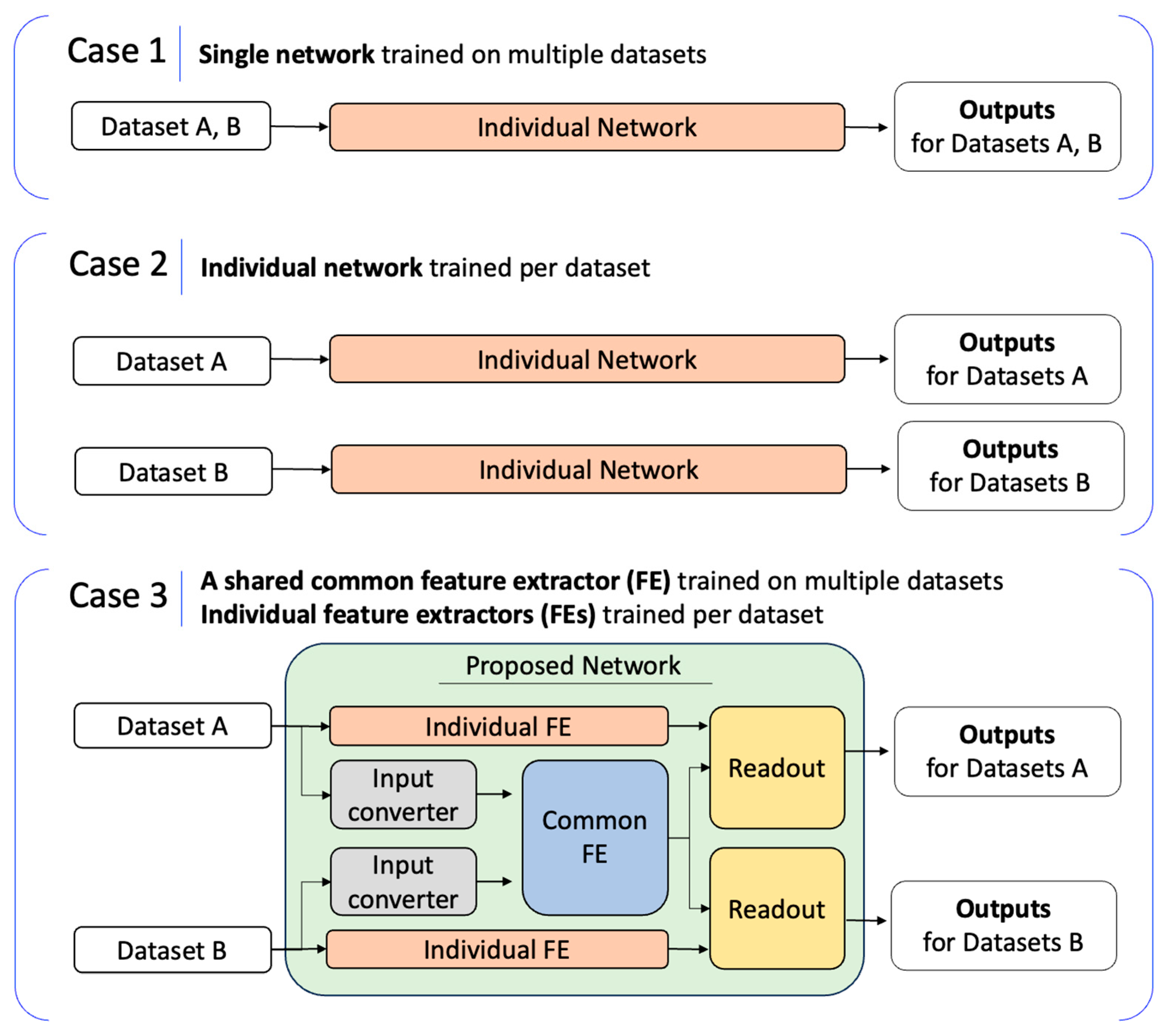
As part of the experiment, three cases were set up to evaluate the effectiveness of the ComFE, as illustrated in Figure 4. In Case 1, all datasets were jointly trained within a single model to extract features across different domains. In Case 2, separate models were trained independently using a single dataset for each, requiring as many models as there were datasets. In contrast, Case 3 employed the proposed architecture with a shared ComFE and multiple IndvFEs, enabling the model to learn common and domain-specific features simultaneously.

The per-domain mini-batch sizes were determined based on the target number of update steps per epoch in the domain-wise training scheme. For each dataset, the batch size was computed by dividing the number of training samples by the target number of steps per epoch, ensuring that most samples were used once per epoch. The target number of steps per epoch was then set to the smallest value that satisfied the GPU memory constraint across all domains, which maximized the feasible batch sizes. Consequently, the batch sizes were set to 100, 146, 120, and 120 for CIFAR10, SVHN, Fashion-MNIST, and MNIST, respectively.

In this experimental setting, we also trained established models—including ResNet50 [29], VGG Net [45], MobileNet v2 [15], EfficientNet v2b0 [16], and ConvNeXt-Tiny [17]—on the same dataset combinations as in Cases 1 and 2. These trained models served as baseline references. The quantitative comparisons are presented in Section 4.

3.5. Hyperparameters

The Adam optimizer was used for all experiments at a learning rate of 1 × 10⁻⁴, which is a commonly adopted setting [46,47]. This learning rate was uniformly applied across all models, including the proposed and baseline architectures, without model-specific tuning. All other hyperparameters followed the default settings provided by the Keras implementations, including the Adam momentum parameters (β₁ = 0.9 and β₂ = 0.999), Glorot-uniform kernel initializer, zero-initialized biases, and absence of regularization. This configuration was adopted to ensure a fair comparison under general training conditions, rather than optimizing the hyperparameters for individual models through empirical tuning. A fixed number of 100 epochs was used for all models to ensure fair comparison across the datasets.

4. Results

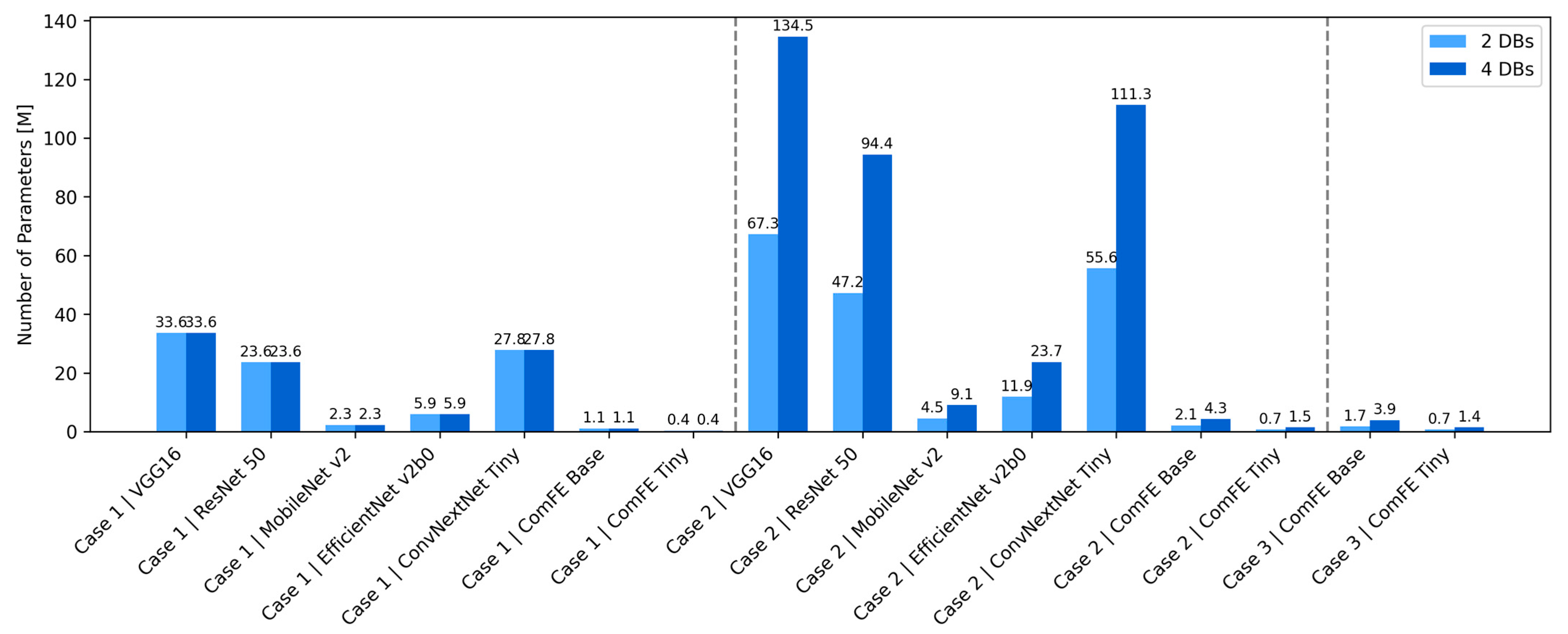
Figure 5 illustrates the number of trainable parameters for all models with different configurations. In Case 1, where a single model was trained on two datasets, the proposed model had approximately 1.07 M parameters—which is significantly fewer than those of VGG16 (33.6 M), ResNet50 (23.6 M), and ConvNeXt-Tiny (27.8 M)—while achieving competitive performance. In Case 2, where individual models were trained for each dataset, the parameter counts doubled. Specifically, the proposed model had 2.1 M parameters, whereas VGG16 had 67.2 M for two datasets and 134.5 M for four datasets. Notably, in Case 3, which incorporated a shared feature extractor, the proposed model had 1.7 M parameters for the two datasets and 3.9 M parameters for the four datasets. Although this value is higher than that in Case 1, it remains significantly lower than those of most conventional models. Compared to MobileNet v2, which has 2.27 M parameters in Case 1, the proposed model is lighter in the two-dataset setting. Although the parameter size increased with the number of datasets, the proposed model in Case 3 still required fewer parameters than MobileNet v2 in Case 2 (4.54 M) and maintained a significantly smaller footprint than the other models. These results demonstrate the scalability of the proposed method, enabling parameter-efficient learning across multiple domains with minimal growth in model size.

Table 2. Classification accuracies for two different dataset pairs (MNIST–FMNIST and CIFAR10–SVHN) in different cases.

Case	Model	MNIST–FMNIST		CIFAR10–SVHN
		MNIST	FMNIST	CIFAR10	SVHN
Case 1	VGG 16	99.32 ± 0.13	92.88 ± 0.35	74.02 ± 0.72	92.63 ± 0.25
	ResNet 50	98.70 ± 0.13	90.06 ± 0.20	57.31 ± 1.28	82.49 ± 1.11
	MobileNet v2	96.45 ± 0.28	86.08 ± 0.35	43.15 ± 0.96	70.00 ± 1.51
	EfficientNet v2b0	83.94 ± 18.37	83.73 ± 6.69	27.24 ± 10.59	46.71 ± 21.60
	ConvNeXt-Tiny	97.93 ± 0.15	88.73 ± 0.40	41.03 ± 14.76	66.68 ± 20.50
	ComFENet-Base	98.71 ± 0.10	90.40 ± 0.52	67.54 ± 1.27	82.82 ± 1.62
	ComFENet-Tiny	94.50 ± 3.05	85.75 ± 1.30	1.46 ± 1.62	15.42 ± 4.12
Case 2	VGG 16	99.50 ± 0.04	92.85 ± 0.33	76.56 ± 0.56	93.66 ± 0.27
	ResNet 50	99.17 ± 0.16	89.83 ± 0.50	58.29 ± 1.24	86.95 ± 0.72
	MobileNet v2	98.25 ± 0.24	85.59 ± 0.48	42.22 ± 0.70	77.42 ± 0.61
	EfficientNet v2b0	72.04 ± 33.28	85.79 ± 8.34	19.82 ± 9.08	77.75 ± 14.18
	ConvNeXt-Tiny	98.89 ± 0.06	91.28 ± 0.27	20.74 ± 14.8	19.59 ± 0.00
	ComFENet-Base	99.02 ± 0.13	91.61 ± 0.56	71.91 ± 1.42	88.22 ± 1.02
	ComFENet-Tiny	91.98 ± 8.04	86.43 ± 4.42	10.00 ± 0.00	6.70 ± 0.00
Case 3	ComFENet-Base	98.28 ± 0.11	89.38 ± 0.55	71.13 ± 0.81	87.94 ± 1.01
	ComFENet-Tiny	94.75 ± 3.19	89.51 ± 0.84	9.98 ± 0.02	72.56 ± 1.57

reports the classification accuracies for two dataset pairs (MNIST–FMNIST and CIFAR10–SVHN) over 10 trials. The results show distinct accuracy characteristics between the two configurations of the proposed model (Base and Tiny). In Case 1, the Base model achieved stable and competitive accuracies across all datasets, whereas the Tiny model showed lower accuracies, particularly on CIFAR10 and SVHN.

The ComFENet-Base model consistently achieved strong and stable accuracy across datasets, showing performance comparable to that of large conventional architectures, such as VGG16 and ResNet-50, while remaining more reliable than lightweight baselines. In particular, in Case 3, ComFENet-Base maintained high accuracy on all datasets (98.87% on MNIST, 91.00% on FMNIST, 68.87% on CIFAR10, and 85.83% on SVHN), despite a substantial reduction in the number of parameters enabled by the shared module. This result indicates that the shared representation effectively reduced the model size without severely degrading the classification performance.

In contrast, ComFENet-Tiny exhibited a stronger dependency on both the dataset characteristics and training configuration. On MNIST, the accuracy remained lower than that of conventional models (e.g., 94.50% in Case 1 and 87.41% in Case 3), whereas on FMNIST, the accuracy was comparable to that of lightweight baselines, reaching 85.75% and 89.29% in Cases 1 and 3, respectively. Notably, this improvement on FMNIST occurred although the model was trained with a smaller model size, suggesting that the shared representation can still contribute positively for simpler datasets.

For more complex datasets, such as CIFAR10 and SVHN, ComFENet-Tiny failed to converge in Cases 1 and 2, yielding near-chance performance (e.g., 1.46% on CIFAR10 and 15.42% on SVHN in Case 1). This behavior implies that aggressive parameter reduction through depthwise convolutions limits the model’s capacity to learn discriminative features when trained on limited dataset combinations. However, when all datasets were jointly used in Case 3, ComFENet-Tiny achieved a substantial improvement in SVHN, reaching an accuracy of 72.56%. This result suggests that the proposed ComFE framework successfully extracts shared representations across different datasets, which can partially compensate for the reduced model capacity and enable effective learning under multi-dataset training conditions.

Table 3. Classification accuracies of the four datasets when all datasets are jointly trained. The results for Case 2 are also included for comparison, although the values are identical to those in Table 2 because of the separate training setting.

Case	Model	MNIST	FMNIST	CIFAR10	SVHN
Case 1	VGG 16	99.20 ± 0.09	92.39 ± 0.27	71.11 ± 0.62	91.37 ± 0.60
	ResNet 50	98.61 ± 0.15	89.67 ± 0.35	57.30 ± 1.04	82.95 ± 2.25
	MobileNet v2	96.62 ± 0.40	85.28 ± 0.44	43.24 ± 1.31	70.13 ± 1.80
	EfficientNet v2b0	89.21 ± 19.93	77.98 ± 16.08	38.05 ± 9.19	65.30 ± 14.18
	ConvNeXt-Tiny	97.97 ± 0.12	88.44 ± 0.41	45.18 ± 0.99	77.42 ± 1.03
	ComFENet-Base	98.28 ± 0.11	89.38 ± 0.55	60.94 ± 1.37	76.31 ± 3.22
	ComFENet-Tiny	0.47 ± 0.58	0.58 ± 0.71	0.25 ± 0.29	9.77 ± 3.02
Case 2	VGG 16	99.50 ± 0.04	92.85 ± 0.33	76.56 ± 0.56	93.66 ± 0.27
	ResNet 50	99.17 ± 0.16	89.83 ± 0.50	58.29 ± 1.24	86.95 ± 0.72
	MobileNet v2	98.25 ± 0.24	85.59 ± 0.48	42.22 ± 0.70	77.42 ± 0.61
	EfficientNet v2b0	72.04 ± 33.28	85.79 ± 8.34	19.82 ± 9.08	77.75 ± 14.18
	ConvNeXt-Tiny	98.89 ± 0.06	91.28 ± 0.27	20.74 ± 14.8	19.59 ± 0.00
	ComFENet-Base	99.02 ± 0.13	91.61 ± 0.56	71.91 ± 1.42	88.22 ± 1.02
	ComFENet-Tiny	91.98 ± 8.04	86.43 ± 4.42	10.00 ± 0.00	6.70 ± 0.00
Case 3	ComFENet-Base	98.87 ± 0.18	91.00 ± 0.29	68.87 ± 2.62	85.83 ± 2.89
	ComFENet-Tiny	87.41 ± 19.16	89.29 ± 1.83	70.09 ± 0.75	76.05 ± 1.21

presents the accuracies of the proposed and other models in three different cases when they were trained and tested on all four datasets. The ComFENet-Base model exhibited performance comparable to that of large, conventional architectures across all datasets. In particular, while ResNet-50 showed relatively lower accuracy on CIFAR10, the Base model achieved a performance comparable to that of VGG16, attaining 68.87% on CIFAR10 and 85.83% on SVHN in Case 3. For MNIST and FMNIST, the accuracies (98.87% and 91.00%, respectively) were similar to those of ResNet-50 in Case 1. Notably, these results were obtained with 83.5% fewer parameters, indicating that the proposed shared-dataset-specific structure can preserve a strong classification performance while significantly reducing the model size.

In contrast, the ComFENet-Tiny model exhibited a dataset-dependent behavior. As indicated in Table 2, the learning process did not converge properly on CIFAR10 and SVHN in Cases 1 and 2. In addition, MNIST and FMNIST failed to converge when CIFAR10 and SVHN were jointly included, indicating a strong influence from the more complex datasets. However, when the ComFE framework was applied in Case 3, the Tiny model achieved substantial performance improvements, exceeding EfficientNet v2b0 and reaching accuracies of 70.09% on CIFAR10 and 76.05% on SVHN. Notably, the accuracy on CIFAR10 was even higher than that of the Base model. These results suggest that the proposed ComFE framework enables effective learning of shared representations across different datasets. Nevertheless, a performance drop was observed on MNIST for the Tiny model in Case 3. This drop appears to be associated with reduced training stability, as reflected by the larger trial-to-trial variability (±19.16) and lower mean accuracy.

5. Discussion

In addition to classification accuracy, the number of trainable parameters is a critical factor in evaluating the practicality of a model. The proposed Base model in Case 3 used only 3.9 M parameters, and the Tiny configuration further reduced the count to 1.4 M. These values were significantly smaller than those of VGG16 (33.6 M), ResNet50 (23.6 M), and ConvNeXt Tiny (27.8 M). Despite this reduction, the Base model delivered competitive accuracy across the datasets. Although MobileNet v2 had fewer parameters (2.27 M) in Case 1, its accuracy was substantially lower, particularly for CIFAR-10 (43.24%) and SVHN (70.13%).

Despite the significantly reduced parameter count, the proposed Base model achieved high accuracy across multiple datasets: 98.87% on MNIST, 91.00% on FMNIST, 68.87% on CIFAR-10, and 85.83% on SVHN. Compared to VGG16, which has 33.6 M parameters, the proposed model achieved a comparable accuracy (2.38%p lower on average across four datasets) with 88.4% fewer parameters. Similarly, compared to ResNet50, which has 23.6 M parameters and achieved accuracies of 98.61% on MNIST, 89.67% on FMNIST, 57.30% on CIFAR-10, and 82.95% on SVHN, the proposed model delivered equivalent or superior performance (4.01%p higher on average across four datasets). Most notably, in Case 3, the proposed Base model outperformed MobileNet v2 (2.3 M) and EfficientNet v2b0 (5.9 M) by 10.27% and 22.29%, respectively. This highlights the efficiency of the proposed model in maintaining high accuracy while significantly reducing its size.

The proposed architecture adopts a parallel structure with multiple feature-extraction modules, namely a ComFE and IndvFEs. The integration of these modules was designed to balance the extraction of domain-specific features with the identification of shared characteristics. Consequently, the proposed architecture improved generalization across multiple datasets while maintaining a lightweight structure. The proposed models generally achieved higher accuracy in Case 3 than in Case 1, implying that the shared module effectively supported joint learning across multiple datasets. For example, for the Base model, which was trained on all four datasets, the average accuracy increased from 81.23% in Case 1 to 86.14% in Case 3. This effect is particularly evident in the Tiny configuration, where datasets that failed to converge in Cases 1 and 2 showed substantial performance improvements when trained jointly. For example, the CIFAR10 accuracy of the Tiny model increased from near-random performance to 70.09% when all four datasets were used, suggesting that the shared module enables effective learning of common representations, even under limited model capacity.

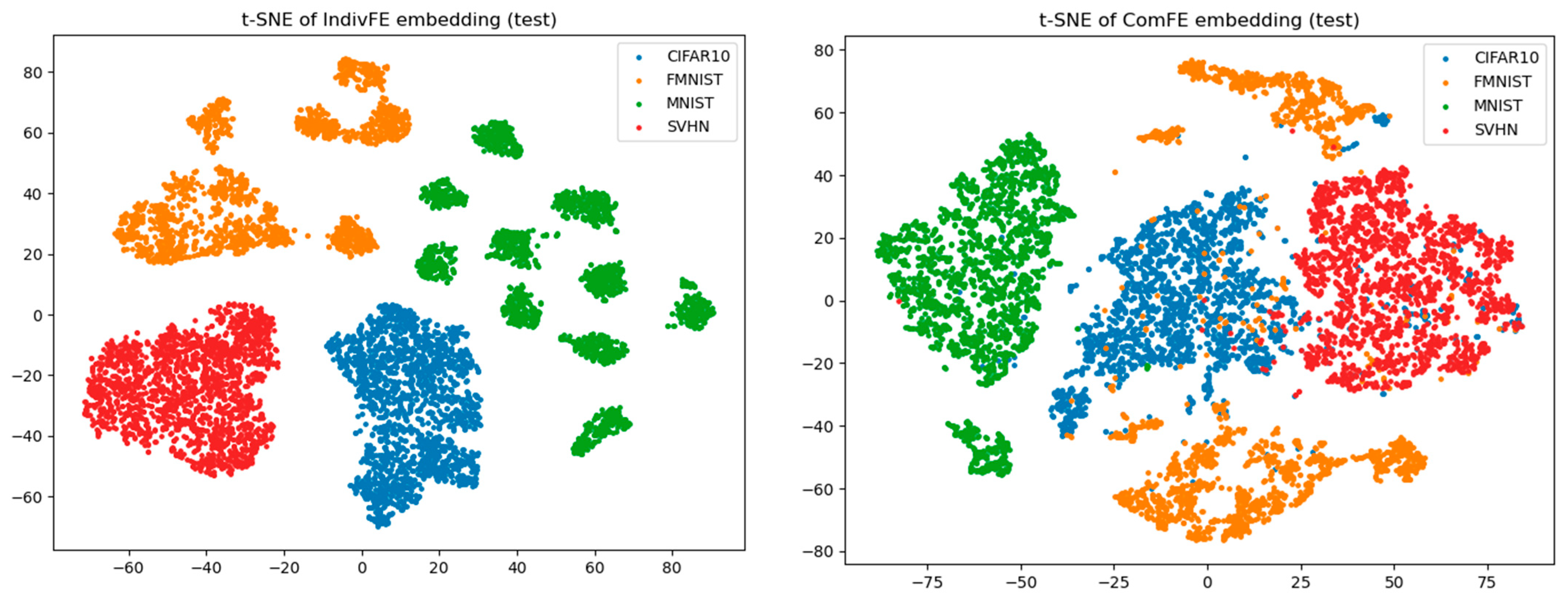
To qualitatively compare the representations learned by the shared and individual modules in Case 3, we visualized the ComFE and IndivFE embeddings of the ComFENet-Tiny model using t-distributed stochastic neighbor embedding (t-SNE), as shown in Figure 6. The t-SNE visualizations indicate that both the ComFE and IndivFE embeddings formed group-wise structures corresponding to each dataset, suggesting that distinctive dataset-related features were captured in both representations. However, the degree of separation clearly differed between these groups. While the IndivFE embeddings exhibited relatively well-separated clusters with limited overlap, reflecting the extraction of dataset-specific characteristics, the ComFE embeddings showed numerous samples distributed across overlapping regions between groups. This increased overlap suggests that the shared module learns representations that are less domain-dependent and emphasizes common features across datasets while preserving a partial group-level structure. For clarity of visualization, t-SNE was applied to a randomly selected subset of 2000 test samples per dataset.

This study did not include separate hyperparameter tuning during the model training. Various optimization-based approaches, such as the improved firehawk optimizer [48] and improved opposition-based particle swarm optimization [49], have shown strong performance in searching hyperparameter spaces. Building on these methods, future studies should consider applying hyperparameter tuning to enhance the performance of the proposed model.

The proposed framework can be viewed as a form of co-learning in which two distinct tasks—domain-invariant and domain-specific feature extractions—are trained within a single network. In related studies, two loss functions corresponding to distinct tasks were jointly optimized within a shared encoder [50]. Alternatively, a unified backbone can be used to generate features separately for classification and localization tasks [51]. In contrast, our model introduces a set of parallel feature extractors (ComFE and IndvFE) that are explicitly designed to separate and learn shared and individual representations. This structural differentiation offers a new perspective on co-learning, and future extensions could explore more diverse loss functions and integration strategies between ComFE and IndvFE to improve accuracy.

The impact of the proposed method varied depending on the number and combination of the datasets used. When the four datasets were trained in the proposed network, the accuracy of the Base model slightly increased for MNIST (0.59%p) and FMNIST (1.62%p) but decreased for CIFAR-10 (−2.26%p) and SVHN (−2.11%p). This reduction suggests that the complexity introduced by the additional datasets may require further optimization with a limited number of parameters. Future research should focus on refining the model architecture to address potential performance degradation when scaling to a larger number of datasets.

To facilitate a direct comparison of the performance attributable to the proposed sharing module, the training processes were conducted without involving the pretraining stages. Consequently, the accuracy levels for CIFAR-10 and SVHN, typically employing pretrained models, were lower than those reported in the recent literature. Unlike traditional methods, such as knowledge distillation and pruning, which require large pre-trained models, our approach learns common features directly from multiple datasets, enhancing the model’s flexibility and performance on new, unseen data. However, to surpass the performance of the pretrained models, further research is necessary to determine the optimal number of datasets and the amount of data required. Identifying these thresholds will help maximize the potential of the model and ensure a robust performance across diverse domains.

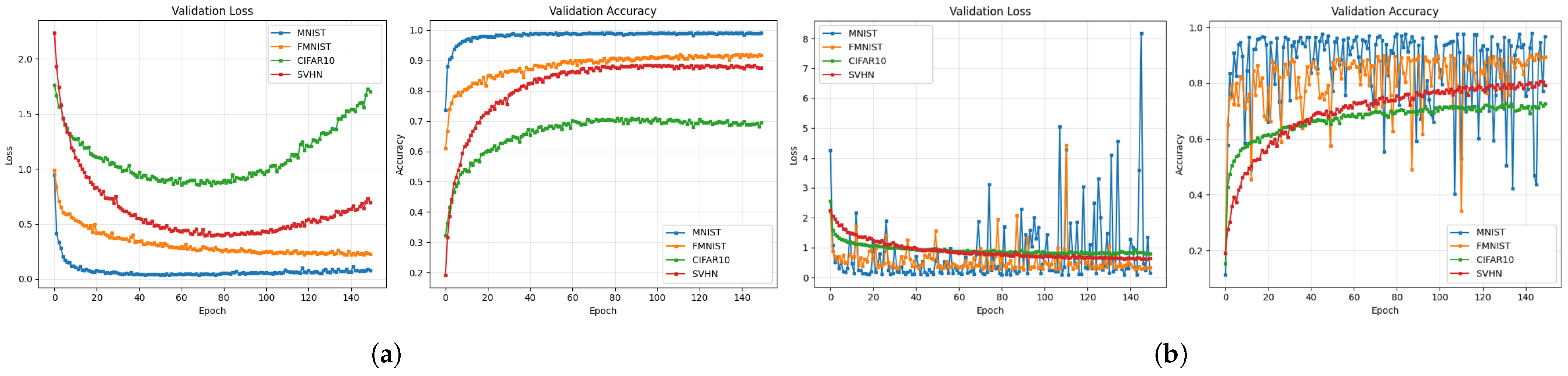
To further analyze the training stability, the training dynamics of the proposed architecture were examined when the four datasets were jointly trained under Case 3. The ComFE-Base model exhibited stable optimization behavior across datasets, achieving consistently high validation accuracy (Figure 7a). Notably, the validation loss for CIFAR10 and SVHN increased after approximately 70 epochs; however, this change did not degrade the validation accuracy, suggesting that the learned decision boundaries remained stable despite slight shifts in confidence calibration. In contrast, the ComFE-Tiny model exhibited pronounced loss fluctuations during training, particularly for MNIST and FMNIST (Figure 7b), indicating an increased sensitivity to optimization noise owing to its reduced capacity. Across all experiments described in Section 4, all models were trained for a fixed 100 epochs to maintain a consistent experimental protocol; however, the observed training dynamics implied that this schedule was not necessarily optimal, particularly for the Tiny variant. Improving training stability through refined optimization strategies and architectural adjustments remains an important direction for future research.

Table 4. Comparison of FLOPs across models and training configurations.

Models	Training Configuration	FLOPs Evaluation Test	Inference FLOPs (M)
VGG16	-	-	664.6
ResNet 50	-	-	158.4
MobileNet v2	-	-	12.6
EfficientNet v2b0	-	-	31.9
ConvNeXt-Tiny	-	-	179.2
ComFE-Base	MNIST–FMNIST	MNIST, FMNIST	1152.4
	CIFAR10–SVHN	CIFAR10, SVHN	1506.8
	All datasets	MNIST, FMNIST	1152.4
	All datasets	CIFAR10, SVHN	1330.3
ComFE-Tiny	MNIST–FMNIST	MNIST, FMNIST	54.6
	CIFAR10–SVHN	CIFAR10, SVHN	72.0
	All datasets	MNIST, FMNIST	54.6
	All datasets	CIFAR10, SVHN	63.5

compares the computational complexities of the proposed ComFE models and conventional architectures in terms of FLOPs. Given the minimum input-size constraint in the Keras implementations, conventional architectures were evaluated using a standard 32 × 32 × 3 input. The proposed ComFE models were evaluated under different training and evaluation configurations, including two-dataset (MNIST–FMNIST and CIFAR10–SVHN) and four-dataset settings, and the results are reported separately for each evaluation dataset. All FLOPs corresponded to single-sample forward inference and reflected the total computational cost of the complete model, including the shared and dataset-specific modules.

The results demonstrate that ComFE-Tiny achieved substantially lower computational complexity than conventional architectures, whereas ComFE-Base incurred higher FLOPs owing to the increased capacity of the shared representation. Notably, for a given evaluation dataset, the FLOPs remained consistent regardless of whether the model was trained on two or all four datasets, indicating that the inference complexity was primarily determined by the dataset-specific input configuration rather than the number of datasets used during training.

ComFE-Tiny exhibited a moderate computational footprint within the spectrum of lightweight architectures. Specifically, it was substantially more efficient than large conventional models, such as VGG16 (664.6 M FLOPs), and smaller than ConvNeXt-Tiny (179.2 M FLOPs), while remaining heavier than ultra-lightweight architectures optimized for mobile deployment, such as MobileNet v2 (12.6 M FLOPs) and EfficientNet v2b0 (31.9 M FLOPs). ComFE-Tiny trained on all datasets required 54.6 M FLOPs for MNIST/FMNIST and 63.5 M FLOPs for CIFAR10/SVHN, which were lower than the 72.0 M FLOPs observed when trained only on CIFAR10–SVHN. This reduction was due to the all-dataset setting, where the shared module used a smaller input size dictated by the lowest-resolution datasets.

When considered together with the accuracy results presented in Table 3, ComFENet-Tiny offered a favorable efficiency–performance trade-off in the four-dataset setting of Case 3. Specifically, it maintained reasonable accuracy across datasets (e.g., 70.09% on CIFAR10 and 76.05% on SVHN) while requiring only 54.6–63.5 M FLOPs, which was approximately one-third of that required by ConvNeXt-Tiny (179.2 M FLOPs).

The proposed model has a clear advantage over existing multi-domain or multi-task learning methods in terms of architectural simplicity and parameter efficiency. Methods such as cross-stitch networks [52] and adapters [53] often introduce additional coupling modules or rely on large pretrained backbones, increasing complexity and computational cost. Parameter-sharing approaches [54] have been predominantly studied and applied in conjunction with large backbone models, where sufficient capacity is assumed to accommodate multiple tasks or domains. In contrast, the proposed model focuses on investigating parameter sharing across multiple small-scale and heterogeneous datasets, explicitly separating shared and domain-specific feature extractors, and training the model from scratch. This design makes the proposed approach particularly suitable for lightweight settings. A systematic comparison with representative multi-domain methods under unified conditions will be explored in future studies.

This study did not thoroughly address class imbalance, which warrants further investigation to improve the performance of the proposed model. Although the employed datasets exhibited only minor differences in sample counts across classes, class imbalance should be considered in future experiments. The domain shift was addressed at the architectural level by separating the shared and individual feature extractors, which enabled the model to learn both common and domain-specific representations and led to improved performance through the shared module. In addition, ComFE was trained and evaluated only on the domains included in the training set and was not tested on a completely unseen dataset (e.g., zero-shot transfer). Therefore, the current results do not directly demonstrate domain invariance in a strict zero-shot sense. Evaluating ComFE on unseen domains is an important direction for future research.

Furthermore, the proposed model was validated only on relatively small-scale benchmark datasets. Consequently, further evaluation on larger and more diverse datasets is required to assess the scalability and general applicability. Explicit robustness tests, such as those involving distribution shifts or corrupted inputs, were not conducted in this study. Systematic robustness evaluations will be explored in future studies.

6. Conclusions

Training a single network model on multiple datasets often requires a large-scale architecture, which can easily degrade the performance of the network compared to building multiple separate models. In contrast, utilizing multiple models requires a system with a larger GPU memory size owing to the large number of network parameters, which can be a burden on embedded systems.

In this study, we propose a network architecture with a parallel structure of convolutional layers to build a lightweight model that is suitable for diverse datasets. The proposed model employs a ComFE to train multiple datasets across different domains. The ComFE, a network module shared by multiple networks, learns the common features of all the datasets. By enabling this module to learn the common features among the datasets, the network size can be reduced compared with that obtained using multiple networks.

The proposed model was verified using four datasets from various domains. It efficiently learned common features while minimizing the number of parameters. The proposed ComFENet-Base model achieved an accuracy comparable to that of ResNet-50, while outperforming lightweight alternatives such as EfficientNet and MobileNet in several settings. ComFENet-Tiny further reduced the model size and computational cost, providing a practical low-resource option in the multi-dataset setting.

Despite these promising results, the proposed method has several limitations. Its performance varies depending on the number and combination of datasets, and joint training on multiple datasets occasionally leads to reduced accuracy, indicating the need for further architectural refinement. Because the experiments were conducted on relatively small datasets, further validation on larger and more diverse datasets is required to fully assess the scalability of the proposed approach. In addition, the proposed models were validated using a specific set of datasets, namely, numeric digit and single-object image classification datasets. The applicability of the proposed framework to other domains, such as natural language processing and time-series analysis, requires further investigation.

Future work will explore structural modifications to the proposed network, such as relaxing the symmetric design between shared and individual modules to better balance the representation capacity. In parallel, we will investigate strategies to stabilize training across diverse dataset combinations, which is critical for reliable multi-dataset learning. The proposed architecture exhibits high scalability because the structure of the internal architectures can be easily adjusted. Additionally, enhancing the learning process by diversifying the loss function could help improve training efficiency and robustness across domains.