Supply Chain with Customer-Based Two-Level Credit Policies under an Imperfect Quality Environment


Abstract
:1. Introduction and Literature Overview
Literature Overview
2. Analytical Model
2.1. Assumptions
- (1)
- The replenishment rate is finite. The lot received by the whole seller contains a certain proportion of defectives. The inspection process is imperfect and leads to Type-I and Type-II errors. The inspection rate is higher than the demand rate.
- (2)
- The demand rate is constant, uniform, and deterministic. The demand is satisfied with perfect items only. The time period is infinite, and the lead time is negligible.
- (3)
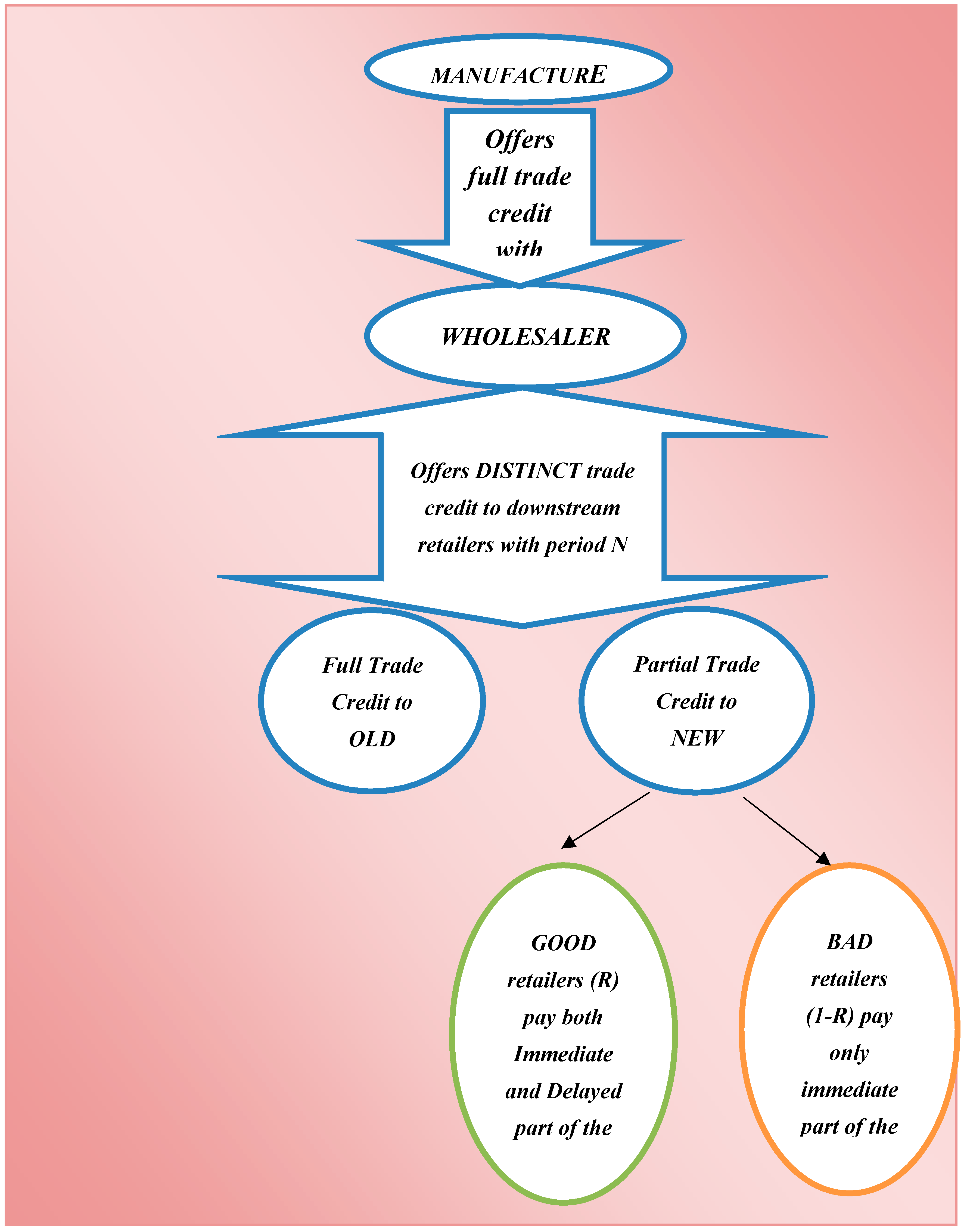
- In the upstream supply chain, a full trade credit policy is offered to the whole seller by the manufacturer. In the downstream supply chain, full trade credit is provided to all old retailers, while partial trade credit is given to all new retailers by the whole seller.
- (4)
- New retailers are categorized into good and bad types, based on their paying/not paying of complete dues on time, respectively. Bad debts are obtained by the fraction of new retailers who fail to pay for the delayed part of the partial trade credit.
- (5)
- Shortages are allowed, and they are fully backlogged.
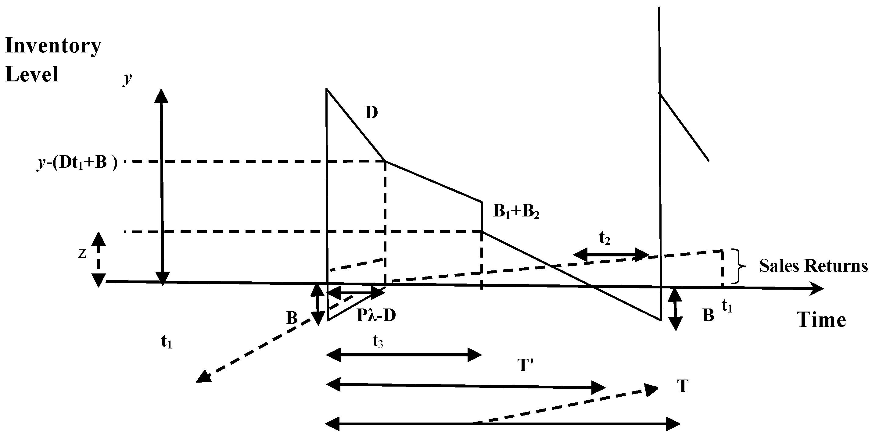
2.2. Problem Description
2.3. Mathematical Modeling
2.3.1. Relevant Costs
- (i)
- Setup cost, which includes the fixed cost per cycle, i.e.:
- (ii)
- Purchase cost which includes variable cost per cycle, i.e.:
- (iii)
- Inspection cost, which includes the cost of inspections per cycle, i.e.:
- (iv)
- Type-I error cost, which includes the cost of rejecting a perfect item, i.e.:
- (v)
- Type-II error cost, which includes the cost of accepting an imperfect item, i.e.:
- (vi)
- The inventory holding cost is the cost of carrying all non-defectives and defective items, plus the items returned from the market, i.e.:
- (vii)
- Backordering cost is the cost of the total shortages that have occurred, i.e.:
2.3.2. Sales Revenue
- (i)
- The sales from sorted perfect items is:
- (ii)
- Revenue loss from sales return:
- (iii)
- Revenue loss from bad debts:
- (iv)
- Sales from total scrap items:
2.3.3. Expected Total Profit per Unit Time
| Case (i) M ≤ N ≤T’ ≤ T | Case (v) N ≤ t3 + N ≤ M ≤ T + N |
| Case (ii) T ≤ M ≤ N | Case (vi) N ≤ T ≤ M ≤ T + N ≤ T + N |
| Case (iii) N ≤ M ≤ t1 ≤ t1 + N ≤ T + N | Case (vii) N ≤ T + N ≤ M ≤ T + N |
| Case (iv) N ≤ t1 + N ≤ M ≤ t3 + N ≤ T + N | Case (viii) N ≤ T’ + N ≤ T + N ≤ M |
3. Theoretical Results for Optimality
4. Solution Procedure
- Step 0:
- Input all parameters.
- Step 1:
- Determine the optimal values of y*, B* for Case (i) from Equations (114) and (115), respectively. Using y*, calculate the corresponding value of t3* and T* from Equations (3) and (10), respectively. If M ≤ N ≤ T’≤ T, then calculate E[Z1(y, B)] from Equation (39), and go to Step 8,otherwise go to Step 2.
- Step 2:
- Determine the optimal values of y*, B* for Case (ii) by substituting the particular values of Gi’s (i = 7,…,12) in Equations (114) and (115), respectively. Using y*, calculate the corresponding value of t3* and T* from Equations (10) and (3), respectively. If T ≤ M ≤ N, then calculate E[Z2(y, B)] from Equation (50) and go to Step 8; else, go to Step 3.
- Step 3:
- Determine the optimal values of y*, B* for Case (iii) by substituting the particular values of Gi’s (i= 13,…,18) in Equations (114) and (115), respectively. Using y*, calculate the corresponding value of t3* and T* from Equations (10) and (3), respectively. If N ≤ M ≤ t1≤ t1 + N ≤ T + N, then calculate E[Z3(y, B)] from Equation (61) and go to Step 8; else, go to Step 4.
- Step 4:
- Determine the optimal values of y*, B* for Case (iv) by substituting the particular values of Gi’s (i =19,…,24) in Equations (114) and (115), respectively. Using y*, calculate the corresponding value of t3* and T* from Equations (10) and (3), respectively. If N ≤ t1 + N ≤ M ≤ t3 + N ≤ T + N, then calculate E[Z4(y, B)] from Equation (72) and go to Step 8; else, go to Step 5.
- Step 5:
- Determine the optimal values of y*, B* for Case (v) by substituting the particular values of Gi’s (i = 25,…,30) in Equations (114) and (115), respectively. Using y*, calculate the corresponding value of t3* and T* from Equations (10) and (3), respectively. If N ≤ t3 + N ≤ M ≤ T’ + N ≤ T + N, then calculate E[Z5(y, B)] from Equation (83) and go to Step 8; else, go to Step 6.
- Step 6:
- Determine the optimal values of y*, B* for Case (vi) by substituting the particular values of Gi’s (i = 31,…,36) in Equations (114) and (115), respectively. Using y*, calculate the corresponding value of t3* and T* from Equations (10) and (3), respectively. If N ≤ T’ ≤ M ≤ T’+N ≤ T+N, then calculate E[Z6(y, B)] from Equation (94) and go to Step 8; else, go to Step 7.
- Step 7:
- Determine the optimal values of y*, B* for Case (vii) by substituting the particular values of Gi’s (i = 37,…,42) in Equations (114) and (115), respectively. Using y*, calculate the corresponding value of t3* and T* from Equations (10) and (3), respectively. If N ≤ T’+N ≤ M ≤ T+N, then calculate E[Z7(y, B)] from Equation (105) and go to Step 8.
- Step 8:
- Procedure terminates.
5. Numerical Analysis
5.1. Numerical Experiments
5.2. Sensitivity Analysis
- As exhibited from Table 5, the optimal values of the order quantity (y*), the backorder level (B*), the cycle length (T*), and the expected value of the total profit per unit time (Z*(y, B)) show a decreasing trend, while the values of the total revenue per unit time and the total cost per unit time increase with the defect proportion (α). The only portion of the revenue being increased with a rise in the number of defectives is from the sale of the scrap items. However, the total cost majorly increases, due to the holding cost and the sales returns cost. With the increased count of the defectives in the system, the demand decreases, due to the frustration in retailers dealing with the faulty items, resulting in the loss of orders and shortages.
- From Table 6, it is observed that with an increase in the proportion of Type-I errors (q1), the optimal values of backorder level (B*), cycle length (T*), and the expected value of total profit per unit time (Z*(y, B)) show declining trends, while the order quantity (y*) increases along with total revenue and total cost values. The Type-I error causes a direct financial loss to the whole seller as his inspection team discards some perfect items at a reduced price, leading to a fall in profit values and cycle length. The increase in the sale of salvage items majorly contributes to raising the revenue. In order to satisfy the demand with perfect items, the whole seller needs to order more; hence, the purchase cost, inspection cost, Type-1 error cost, and holding costs increases with the rise in the value of (y)*. Further, with a higher number of orders, there is a lessening of shortages as the demand can now be satisfied in a better way.
- It is clear from Table 7 that with an increment in the proportion of Type-II errors (q2), the optimal values of order quantity (y*), cycle length (T*), and expected value of the total profit per unit time (Z*(y, B)), and the total revenue exhibit a declining nature, while the optimal backorder level (B*), and total cost values show a rise. The Type-II error causes a penalty and goodwill loss to the whole seller by the sale of some defectives to the retailers, resulting in sales returns. Because of these defect returns, there is an addition to the inventory of the system, leading to increase in holding cost and Type-II error cost. Owing to frustration and quality dissatisfaction, the retailers may not be willing to purchase more, so a decrement is observed in the values of (y)*, and thus in the total profit of the system. Due to the lack of purchases made, there is an increase in backorder level, i.e., (B)*.
- With the increase in the proportion of initial payments (δ), there is a lowering of order quantity (y*), while there is increase in the optimal values of the expected total profit per unit time (Z*(y, B)), backorder level (B*), cycle length (T*), and total cost. An increase in the initial partial payment leads to a reduction in the number of retailers who are interested in bulk purchases, majorly due to the discount/credit offered. With lesser demand come fewer orders and a shortening of the cycle length. However, due to an elevation in the fraction of initial payments, it becomes more profitable for the whole seller, as he can now generate extra revenue by keeping the additional amounts in an interest-bearing account.
- With a growth in the proportion of old retailers (K), the optimal values of order quantity (y*) and cycle length (T*) decrease, while the optimal values of the expected total profit per unit time (Z*(y, B)), and backorder level (B*) show increasing behaviors. With the higher value of (K), the whole seller is able to offer full permissible delays to a greater number of retailers, resulting in his increased profit values. However, since the y* values are found to decrease, this implies that the whole seller cannot rely on old retailers fully to achieve maximum possible sales, but should focus on promoting new retailers simultaneously.
- It is evident that an enhancement in the proportion of good retailers (R) increases the optimal values of the expected total profit per unit time (Z*(y, B)), backorder level (B*), and total cost, while reducing the optimal values of order quantity (y*) and cycle length (T*) slightly. With an increasing number of good retailers, who make complete partial payments, the whole seller is able to minimize his losses that directly occur due to bad debts, and hence, his profit values rise. The order quantity and cycle length reveal a marginal decreasing trend, owing to the fact that the whole seller is interested in ordering less but more frequently to achieve the target sales.
- Upon increasing the whole seller’s credit period (M), the optimal values of the expected total profit per unit time (Z*(y, B)), backorder level (B*), and total cost increase, while the optimal values of order quantity (y*) and cycle length (T*) decrease. With the increase of the whole seller’s credit limit, he is able to put the revenue generated through sales into an interest-bearing account for a longer duration, and hence boost up his profit values considerably. However, with a reduction in the order quantity, there will be higher number of customers waiting for delivery, i.e., there is an increase in backorder levels.
- The higher credit limit of retailers (N), the less are the optimal values of the expected total profit per unit time (Z*(y, B)), backorder level (B*), cycle length (T*), order quantity (y*), and total cost. When the first payment to the whole seller is delayed, he is unable to put revenue into his account for a longer period, thus affecting his profit values negatively. With larger N, the major source of revenue generation comes from the immediate payments by all the new retailers. The whole seller experiences a reduction in the order quantity to avoid a larger risk being attached to the bad credit retailers who do not pay the remaining part of the partially permissible delay at N.
6. Summary
6.1. Managerial Insights
6.2. Concluding Remarks
6.3. Future Research and Limitations
Author Contributions
Funding
Conflicts of Interest
Nomenclature
| Index | |
| j | number of cases (j=1, 2, 3, 4, 5, 6, 7) |
| Parameters | |
| D | demand rate in units per unit time (units/time) |
| λ | inspection rate in units per unit time, λ > D |
| A | proportion of imperfect items (a random variable with known probability density function) |
| q1 | proportion of Type-I imperfection errors (a random variable with known probability density function) |
| q2 | proportion of Type-II imperfection errors (a random variable with known probability density function) |
| E(.) | expected value operator |
| E(θ) | expected value of θ |
| A | setup cost for each cycle ($/setup) |
| c | purchase cost per item ($/item) |
| i | inspection cost per item ($/item) |
| s | selling price ($/item) |
| v | salvage cost (<s) ($/item) |
| cr | cost of committing a Type-I error ($/item) |
| ca | cost of committing a Type-II error ($/item) |
| cB | backordering cost per unit per unit time ($/item) |
| H | holding cost per unit time per unit time ($/unit/unit time) |
| δ | fraction of the purchase cost made at the initial time of the credit period |
| K | percentage of old retailers (estimated from the past data) |
| R | percentage of good retailers (estimated from the past data) |
| M | credit period offered by the manufacturer to the whole seller to settle his accounts (time unit) |
| N | credit period offered by the whole seller to the retailers to settle his accounts (time unit) |
| Ie | interest earned per unit per unit time ($/unit/unit time) |
| Ip | interest paid per unit per unit time ($/unit/unit time) |
| f(α) | probability density function of defective items |
| f(q1) | probability density function of Type-I error |
| f(q2) | probability density function of Type-II error |
| Independent Decision variables | |
| y | whole seller’s order lot size for each cycle (units) |
| B | whole seller’s backorder size for each cycle (units) |
| Dependent Decision variables | |
| T | cycle length |
| T.C.U. | whole seller’s total cost per unit time |
| T.R.U. | whole seller’s total revenue per unit time |
| T.P. j | whole seller’s total profit for j |
| Zj(y, B) | whole seller’s total profit per unit time for j |
| E[Zj(y,B)] | whole seller’s expected total profit per unit time for j |
Appendix A
Appendix B
Appendix C
References
- Haley, C.W.; Higgins, R.C. Inventory policy and trade credit financing. Manag. Sci. 1973, 20, 464–471. [Google Scholar] [CrossRef]
- Goyal, S.K. Economic order quantity under conditions of permissible delay in payments. J. Oper. Res. Soc. 1985, 36, 335–338. [Google Scholar] [CrossRef]
- Davis, R.A.; Gaither, N. Optimal ordering policies under conditions of extended payment privileges. Manag. Sci. 1985, 31, 499–509. [Google Scholar] [CrossRef]
- Aggarwal, S.P.; Jaggi, C.K. Ordering policies of deteriorating items under permissible delay in payments. J. Oper. Res. Soc. 1995, 46, 658–662. [Google Scholar] [CrossRef]
- Teng, J.T.; Chang, C.T.; Chern, M.S.; Chan, Y.L. Retailer’s optimal ordering policies with trade credit financing. Int. J. Syst. Sci. 2007, 38, 269–278. [Google Scholar] [CrossRef]
- Su, C.H.; Ouyang, L.Y.; Ho, C.H.; Chang, C.T. Retailer’s inventory policy and supplier’s delivery policy under two-level trade credit strategy. Asia-Pac. J. Oper. Res. 2007, 24, 613–630. [Google Scholar] [CrossRef]
- Jaggi, C.K.; Goyal, S.K.; Goel, S.K. Retailer’s optimal replenishment decisions with credit-linked demand under permissible delay in payments. Eur. J. Oper. Res. 2008, 190, 130–135. [Google Scholar] [CrossRef]
- Huang, Y.F.; Hsu, K.H. An EOQ model under retailer partial trade credit policy in supply chain. Int. J. Prod. Econ. 2008, 112, 655–664. [Google Scholar] [CrossRef]
- Huang, Y.F. Retailer’s inventory policy under supplier’s partial trade credit policy. J. Oper. Res. Soc. Jpn. 2005, 48, 173–182. [Google Scholar] [CrossRef]
- Teng, J.T. Optimal ordering policies for a retailer who offers distinct trade credits to its good and bad credit customers. Int. J. Prod. Econ. 2009, 119, 415–423. [Google Scholar] [CrossRef]
- Jaggi, C.K.; Verma, M. Ordering policies under supplier-retailer partial trade credit financing. Opsearch 2010, 47, 293–310. [Google Scholar] [CrossRef]
- Jaggi, C.K.; Verma, M.; Kausar, A. Customer based two stage credit policies in a supply chain. In Proceedings of the 2011 International Conference on Industrial Engineering and Operations Management, Kuala Lumpur, Malaysia, 22–24 January 2011. [Google Scholar]
- Jaggi, C.K.; Aggarwal, K.K.; Verma, M. Optimal retailer’s ordering policies under two-stage partial trade credit financing in a supply chain. Int. J. Ind. Syst. Eng. 2012, 10, 277–299. [Google Scholar] [CrossRef]
- Taleizadeh, A.A.; Pentico, D.W.; Jabalameli, M.S.; Aryanezhad, M. An EOQ model with partial delayed payment and partial back ordering. Omega 2013, 41, 354–368. [Google Scholar] [CrossRef]
- Giri, B.C.; Sharma, S. Optimal ordering policy for an inventory system with linearly increasing demand and allowable shortages under two levels trade credit financing. Oper. Res. 2016, 16, 25–50. [Google Scholar] [CrossRef]
- Shi, X.; Zhang, S. An incentive-compatible solution for trade credit term incorporating default risk. Eur. J. Oper. Res. 2010, 206, 178–196. [Google Scholar] [CrossRef]
- Tiwari, S.; Ahmed, W.; Sarkar, B. Multi-item sustainable green production system under trade-credit and partial backordering. J. Clean. Prod. 2018, 204, 82–95. [Google Scholar] [CrossRef]
- Wu, J.; Chan, Y.L. Lot-sizing policies for deteriorating items with expiration dates and partial trade credit to credit-risk customers. Int. J. Prod. Econ. 2014, 155, 292–301. [Google Scholar] [CrossRef]
- Chen, S.C.; Teng, J.T. Inventory and credit decisions for time-varying deteriorating items with up-stream and down-stream trade credit financing by discounted cash flow analysis. Eur. J. Oper. Res. 2015, 243, 566–575. [Google Scholar] [CrossRef]
- Shah, N.H. Retailer’s replenishment and credit policies for deteriorating inventory under credit period-dependent demand and bad-debt loss. TOP 2015, 23, 298–312. [Google Scholar] [CrossRef]
- Sarkar, B.; Saren, S. Partial trade-credit policy of retailer with exponentially deteriorating items. Int. J. App. Comput. Math. 2015, 1, 343–368. [Google Scholar] [CrossRef]
- Wu, J.; Al-Khateeb, F.B.; Teng, J.T.; Cárdenas-Barrón, L.E. Inventory models for deteriorating items with maximum lifetime under downstream partial trade credits to credit-risk customers by discounted cash-flow analysis. Int. J. Prod. Econ. 2016, 171, 105–115. [Google Scholar] [CrossRef]
- Mahata, G.C.; De, S.K. Supply chain inventory model for deteriorating items with maximum lifetime and partial trade credit to credit-risk customers. Int. J. Manag. Sci. Eng. Manag. 2017, 12, 21–32. [Google Scholar] [CrossRef]
- Wu, C.; Zhao, Q.; Xi, M. A retailer-supplier supply chain model with trade credit default risk in a supplier-Stackelberg game. Comput. Ind. Eng. 2017, 112, 568–575. [Google Scholar] [CrossRef]
- Porteus, E.L. Optimal lot sizing, process quality improvement and setup cost reduction. Oper. Res. 1986, 34, 137–144. [Google Scholar] [CrossRef]
- Cárdenas-Barrón, L.E.; Sarkar, B.; Treviño-Garza, G. Easy and improved algorithms to joint determination of the replenishment lot size and number of shipments for an EPQ model with rework. Math. Comput. Appl. 2013, 18, 3138–3151. [Google Scholar] [CrossRef]
- Lee, H.L.; Rosenblatt, M.J. Simultaneous determination of production cycle and inspection schedules in a production system. Manag. Sci. 1987, 33, 1125–1136. [Google Scholar] [CrossRef]
- Zhang, X.; Gerchak, Y. Joint lot sizing and inspection policy in an EOQ model with random yield. IIE Trans. 1990, 22, 41–47. [Google Scholar] [CrossRef]
- Salameh, M.K.; Jaber, M.Y. Economic production quantity model for items with imperfect quality. Int. J. Prod. Econ. 2000, 64, 59–64. [Google Scholar] [CrossRef]
- Cárdenas-Barrón, L.E. Observation on: Economic production quantity model for items with imperfect quality. Int. J. Prod. Econ. 2000, 67, 201. [Google Scholar] [CrossRef]
- Goyal, S.K.; Cárdenas-Barrón, L.E. Note on: Economic production quantity model for items with imperfect quality—A practical approach. Int. J. Prod. Econ. 2002, 77, 85–87. [Google Scholar] [CrossRef]
- Papachristos, S.; Konstantaras, I. Economic ordering quantity models for items with imperfect quality. Int. J. Prod. Econ. 2006, 100, 148–154. [Google Scholar] [CrossRef]
- Maddah, B.; Jaber, M.Y. Economic order quantity for items with imperfect quality: Revisited. Int. J. Prod. Econ. 2008, 112, 808–815. [Google Scholar] [CrossRef]
- Raouf, A.; Jain, J.K.; Sathe, P.T. A cost-minimization model for multi characteristic component inspection. AIIE Trans. 1983, 15, 187–194. [Google Scholar]
- Sarkar, B.; Saren, S. Product inspection policy for an imperfect production system with inspection errors and warranty cost. Eur. J. Oper. Res. 2016, 248, 263–271. [Google Scholar] [CrossRef]
- Duffuaa, S.O.; Khan, M. Impact of inspection errors on the performance measures of a general repeat inspection plan. Int. J. Prod. Res. 2005, 43, 4945–4967. [Google Scholar] [CrossRef]
- Khan, M.; Jaber, M.Y.; Bonney, M. An economic order quantity (EOQ) for items with imperfect quality and inspection errors. Int. J. Prod. Econ. 2011, 133, 113–118. [Google Scholar] [CrossRef]
- Sett, B.; Sarkar, S.; Sarkar, B. Optimal buffer inventory and inspection errors in an imperfect production system with regular preventive maintenance. Int. J. Adv. Manuf. Technol. 2017, 90, 545–560. [Google Scholar] [CrossRef]
- Hsu, J.T.; Hsu, L.F. An EOQ model with imperfect quality items, inspection errors, shortage back ordering, and sales returns. Int. J. Prod. Econ. 2013, 143, 162–170. [Google Scholar] [CrossRef]
- Zhou, Y.; Chen, C.; Li, C.; Zhong, Y. A synergic economic order quantity model with trade credit, shortages, imperfect quality and inspection errors. Appl. Math. Model. 2016, 40, 1012–1028. [Google Scholar] [CrossRef]
- Khanra, S.; Mandal, B.; Sarkar, B. An inventory model with time dependent demand and shortages under trade credit policy. Econ. Mod. 2013, 35, 349–355. [Google Scholar] [CrossRef]
- Khanna, A.; Kishore, A.; Jaggi, C. Impact of inflation and trade credit policy in an inventory model for imperfect quality items with allowable shortages. Control Cybern. 2016, 45, 37–82. [Google Scholar]
- Palanivel, M.; Uthayakumar, R. An inventory model with imperfect items, stock dependent demand and permissible delay in payments under inflation. RAIRO-Oper. Res. 2016, 50, 473–489. [Google Scholar] [CrossRef]
- Taleizadeh, A.A.; Lashgari, M.; Akram, R.; Heydari, J. Imperfect economic production quantity model with upstream trade credit periods linked to raw material order quantity and downstream trade credit periods. Appl. Math. Model. 2016, 40, 8777–8793. [Google Scholar] [CrossRef]
- Khanna, A.; Kishore, A.; Jaggi, C. Strategic production modeling for defective items with imperfect inspection process, rework, and sales return under two-level trade credit. Int. J. Ind. Eng. Comput. 2017, 8, 85–118. [Google Scholar] [CrossRef]


| Author(s) | Imperfect Quality | Screening Errors | Credit Policy | Bifurcation of Customer | Bad Debts | Shortages | Optimality | ||
|---|---|---|---|---|---|---|---|---|---|
| Upstream | Downstream | Old and New | Good and Bad | ||||||
| Teng [10] | No | No | Yes (Full) | Yes (Distinct) | No | Yes | No | No | Closed-form |
| Jaggiand Verma [11] | No | No | Yes (Partial) | Yes (Partial) | No | No | No | No | Mathematical |
| Jaggi et al. [12] | No | No | Yes (Full) | Yes (Distinct) | Yes | No | No | No | Closed-form |
| Jaggi et al. [13] | No | No | Yes (Partial) | Yes (Partial) | No | No | No | No | Algebraic |
| Hsu and Hsu [39] | Yes | Yes | No | No | No | No | No | Yes | Closed-form |
| Taleizadeh et. al. [14] | No | No | Yes (Partial) | No | No | No | No | Yes | Closed-form |
| Wu and Chan [18] | No | No | Yes (Full) | Yes (Partial) | No | No | No | No | Mathematical |
| Chang et. al. [41] | Yes | Yes | No | Yes (Full) | No | No | No | No | Mathematical |
| Palanivel and Uthayakumar [43] | Yes | No | Yes (Full) | No | No | No | No | No | Graphical |
| Taleizadeh et. al. [44] | Yes | No | Yes (Full) | Yes (Full) | No | No | No | Yes | Mathematical |
| Sarkar and Saren [21] | No | No | Yes (Full) | Yes (Partial) | No | No | No | No | Mathematical |
| Zhou et. al. [40] | Yes | Yes | Yes (Full) | No | No | No | No | Yes | Closed-form |
| Mahata and De [23] | No | No | Yes (Full) | Yes (Partial) | No | No | No | No | Mathematical |
| Khanna et al. [45] | Yes | Yes | Yes (Full) | Yes (Full) | No | No | No | No | Mathematical |
| This paper | Yes | Yes | Yes (Full) | Yes (Partial) | Yes | Yes | Yes | Yes | Closed-form |
| Cases | Immediate Payment Part | Delayed Payment Part |
|---|---|---|
| Case (i) M ≤ N ≤ T’ ≤ T |  |  |
| Case (ii) T ≤ M ≤ N | 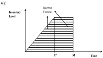 | 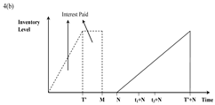 |
| Case (iii) N ≤ M ≤ t1 ≤ t1 + N ≤ T + N |  |  |
| Case (iv) N ≤ t1 + N ≤ M ≤ t3 + N ≤ T + N |  |  |
| Case (v) N ≤ t3 + N ≤ M ≤ T + N |  | 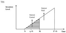 |
| Case (vi) N ≤ T ≤ M ≤ T + N ≤ T + N | 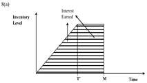 | 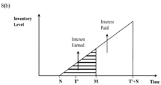 |
| Case (vii) N ≤ T’ + N ≤ M ≤ T + N | 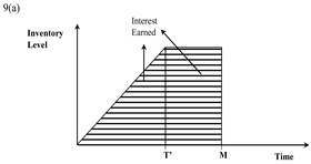 | 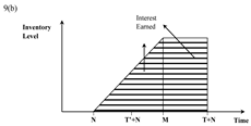 |
| Description | Symbol | Value | Units |
|---|---|---|---|
| Set-up cost | A | 12 | $/cycle |
| Purchase cost | C | 0.5 | $/unit |
| Selling price | s | 1 | $/unit |
| Holding cost | h | 0.2 | $/unit/year |
| Interest earned | Ie | 0.1 | $/year |
| Interest paid | Ip | 0.08 | $/year |
| Description | Symbol | Value | Units |
|---|---|---|---|
| Defect proportion | α | U~(0.5,0.15) | - |
| Type-1 error proportion | q1 | U~(0.1,0.3) | - |
| Type-1 error proportion | q2 | U~(0.1,0.3) | - |
| Probability density function | f(α) | 1/(0.15–0.5) | - |
| Probability density function | f(q1) | 1/(0.3–0.1) | - |
| Probability density function | f(q2) | 1/(0.3–0.1) | - |
| Demand rate | D | 5000 | units/year |
| Inspection rate | λ | 8500 | units/year |
| Inspection cost | i | 0.15 | $/unit |
| Salvage cost | v | 0.35 | $/unit |
| Type-I error cost | cr | 0.05 | $/unit |
| Type-II error cost | ca | 0.1 | $/unit |
| Backorder cost | cB | 0.2 | $/unit/year |
| Fraction of the purchase amount | δ | 20 | % |
| Fraction of old retailers | K | 40 | % |
| Fraction of good retailers | R | 70 | % |
| Whole seller’s credit limit | M | 40 | days |
| Retailer’s credit limit | N | 10 | days |
| Description | Symbol | Value | Units |
|---|---|---|---|
| Order size | y* | 709.47 | units/cycle |
| Backorder quantity | B* | 66.81 | units/cycle |
| Expected total profit per unit time | E[Z*(y, B)] | 663.26 | $/year |
| Cycle length | T* | 45.78 | days |
| q1 | 0 | 0.01 | 0.02 | 0.03 | 0.04 | |
|---|---|---|---|---|---|---|
| y* | ↑ | 708.79 | 708.93 | 709.47 | 710.60 | 712.65 |
| B* | ↓ | 90.01 | 79.28 | 66.81 | 51.84 | 33.03 |
| T* | ↓ | 46.67 | 46.21 | 45.78 | 45.39 | 45.05 |
| Z*(y,B) | ↓ | 705.98 | 684.81 | 663.26 | 641.35 | 619.11 |
| TRU* | ↑ | 4464.52 | 4484.02 | 4503.90 | 4524.22 | 4544.94 |
| R1 | ↓ | 639.32 | 633.08 | 627.17 | 621.77 | 617.15 |
| R2 | ↓ | −1.41 | −1.42 | −1.42 | −1.42 | −1.42 |
| R3 | ↑ | −91.85 | −90.96 | −90.10 | −89.33 | −88.66 |
| R4 | ↑ | 24.80 | 27.05 | 29.30 | 31.58 | 33.92 |
| TCU* | ↑ | 3773.67 | 3814.06 | 3855.10 | 3896.73 | 3938.81 |
| SC | - | 12.00 | 12.00 | 12.00 | 12.00 | 12.00 |
| PC | ↑ | 354.39 | 354.47 | 354.73 | 355.29 | 356.32 |
| IC | ↑ | 106.31 | 106.34 | 106.42 | 106.58 | 106.89 |
| EC1 | ↑ | 0 | 0.32 | 0.63 | 0.95 | 1.28 |
| EC2 | - | 0.14 | 0.14 | 0.14 | 0.14 | 0.14 |
| HC | ↑ | 9.20 | 9.28 | 9.35 | 9.42 | 9.46 |
| BC | ↓ | 0.46 | 0.37 | 0.26 | 0.16 | 0.06 |
| q2 | 0 | 0.02 | 0.03 | 0.04 | 0.05 | |
|---|---|---|---|---|---|---|
| y* | ↓ | 712.66 | 709.47 | 707.90 | 706.34 | 704.80 |
| B* | ↑ | 63.82 | 66.81 | 68.25 | 69.65 | 71.02 |
| T* | ↓ | 45.89 | 45.78 | 45.73 | 45.68 | 45.64 |
| Z*(y,B) | ↓ | 666.57 | 663.26 | 661.61 | 659.97 | 658.33 |
| TRU* | ↓ | 4514.13 | 4503.90 | 4498.82 | 4493.75 | 4488.68 |
| R1 | ↓ | 628.56 | 627.17 | 626.49 | 625.82 | 625.16 |
| R2 | ↓ | 0.00 | −1.42 | −2.12 | −2.83 | −3.52 |
| R3 | ↑ | −90.51 | 90.10 | −89.91 | −89.71 | −89.52 |
| R4 | ↓ | 29.43 | 29.30 | 29.24 | 29.17 | 29.11 |
| TCU* | ↑ | 3861.81 | 3855.10 | 3851.76 | 3848.41 | 3845.08 |
| SC | - | 12.00 | 12.00 | 12.00 | 12.00 | 12.00 |
| PC | ↓ | 356.33 | 354.74 | 353.95 | 353.17 | 352.40 |
| IC | ↓ | 106.90 | 106.42 | 106.19 | 105.95 | 105.72 |
| EC1 | ↓ | 0.64 | 0.64 | 0.64 | 0.64 | 0.63 |
| EC2 | ↑ | 0.00 | 0.14 | 0.21 | 0.28 | 0.35 |
| HC | ↑ | 9.37 | 9.36 | 9.36 | 9.35 | 9.35 |
| BC | ↓ | 0.24 | 0.27 | 0.28 | 0.29 | 0.30 |
© 2018 by the authors. Licensee MDPI, Basel, Switzerland. This article is an open access article distributed under the terms and conditions of the Creative Commons Attribution (CC BY) license (http://creativecommons.org/licenses/by/4.0/).
Share and Cite
Khanna, A.; Kishore, A.; Sarkar, B.; Jaggi, C.K. Supply Chain with Customer-Based Two-Level Credit Policies under an Imperfect Quality Environment. Mathematics 2018, 6, 299. https://doi.org/10.3390/math6120299
Khanna A, Kishore A, Sarkar B, Jaggi CK. Supply Chain with Customer-Based Two-Level Credit Policies under an Imperfect Quality Environment. Mathematics. 2018; 6(12):299. https://doi.org/10.3390/math6120299
Chicago/Turabian StyleKhanna, Aditi, Aakanksha Kishore, Biswajit Sarkar, and Chandra K. Jaggi. 2018. "Supply Chain with Customer-Based Two-Level Credit Policies under an Imperfect Quality Environment" Mathematics 6, no. 12: 299. https://doi.org/10.3390/math6120299
APA StyleKhanna, A., Kishore, A., Sarkar, B., & Jaggi, C. K. (2018). Supply Chain with Customer-Based Two-Level Credit Policies under an Imperfect Quality Environment. Mathematics, 6(12), 299. https://doi.org/10.3390/math6120299