1. Introduction
Fractional models have an important role in many fields of engineering and science, for instance, fluid flows, solute transport, electromagnetic theory, signal processing, biology, economics, physics, and geology, etc. [
1,
2,
3,
4,
5,
6]. Fractional theory has many applications in wireless networks [
7,
8]. Moreover, fractional modeling has been applied in micro-grids [
9], and decentralized wireless networks [
10].
Fractional differential equations (FDEs) involve real or complex order derivatives [
11]. Various researchers contributed on fractional derivatives during the 18th and 19th centuries, for example, Abel [
12], Caputo [
13], Euler [
14], Fourier [
15], Laplace [
16], Liouville [
17], or Ross [
18]. In 1974, Oldham and Spanier presented fractional operators with mass and heat transfer applications [
19]. In this paper, the analytical technique to solve fractional order partial differential equations (PDEs) is described. In order to obtain analytical solution, HPM is used to solve fractional order PDEs. Fractional order PDEs do not have closed form exact solutions in most problems, therefore, it is required to develop efficient and accurate analytical and numerical methods. HPM is well known for its accuracy and simplicity [
20,
21]. HPM has been widely used to obtain approximate series solutions of fractional order linear and nonlinear PDEs [
22,
23,
24,
25,
26,
27].
The Burger Poisson equation is widely used to express different physical phenomena, for instance, mathematical models for shallow water and shock waves in a viscous fluid [
28]. Tian and Gao proved the existence of the uni-dimensional viscous equation in 2009 [
29]. Moreover, Abidi and Omrani obtained the solution of Burger Poisson equation using homotopy analysis method [
30].
The obstacle problem plays a role of bridge in the field of variational inequalities and differential equations. It is originated from the study of elasticity theory. In elasticity theory, it is required to obtain the equilibrium position of elastic membrane with fixed boundaries. Obstacle problems occur in diffusion equation and signals processing while determining heat flux at the boundary of semi-infinite rod [
31].
The focus of the paper is to generalize the convergence theorem, in the sense that the mapping is nonself and only Y is complete. Theorem is applied to the solution of FBP equation acquired by HPM. Furthermore, this work presents the method to get the solution of FPDEs, while the same PDE with ordinary derivative i.e., for is not defined in the given domain. Moreover, the proposed HPM method is applied to complex obstacle BVP.
Beside the introduction, the distribution of the article is as under:
Section 2 comprises of important definitions and properties,
Section 3 contains the implementation of HPM to solve FPDEs and convergence theorem,
Section 4 comprises of results and discussion of FBP,
Section 5 contains solutions of obstacle BVP, and
Section 6 includes the conclusion of the paper.
2. Preliminaries
Fractional calculus is a developing area in mathematical analysis. Several definitions of fractional operators have been propounded like Riemann-Liouvlle, Caputo, and Grunwald-Letnikov [
13,
17]. These definitions have some limitations, for instance
, do not satisfy the product, quotient and chain rules of derivatives. Recently, Khalil et al. published a definition uses for fractional derivatives called conformable [
32,
33]. Conformable is simpler and natural extension of the usual derivatives as it satisfies the aforementioned properties of derivatives.
Definition 1. A function . The fractional derivative of g for order α is given below: If g is -differentiable in , . If exists, then .
The definition given in Equation (1) is known as conformable [33]. Using the above mentioned definition given in Equation (
1), we obtain the following useful results:
Let are -differentiable and , then
If a function is -differentiable at , then g is continuous at .
, for all .
, for all .
, for all constant function .
.
.
If g is differentiable, then .
Fractional integral: The fractional integral of order
can be defined below:
Here,
is the Riemann improper integral.
3. Application of HPM to FBP Equation
Consider the time-dependent operator equation
where
B denotes a differential operator and
is an unknown function. Moreover, we assume
is an analytic function, we can decompose the operator
B as;
where
L is linear and
N is nonlinear or sometimes the complicated part to handle. Let
the homotopy
is defined as:
Note that the function
is the initial guess which satisfies the given operator equation. The choice of
p from zero to one provide us the deformation from
to the solution
. Clearly
and
which is the given operator equation. Using perturbation method, we suppose the solution in power series as;
For
is an approximate solution to the given operator equation.
Remark 1. The Banach contraction type theorem about the convergence of the solution stated in [34]. Here the generalized, corrected, and unified form is presented in which the completeness of X is not required and Y must be a subset of X. If , we cannot say about the sequence is contained in Y or not. On the basis of above discussion, a unified theorem is presented as follows: Theorem 1. Let X be a normed space and Y be a Banach space, be a mapping such that for all for some then the sequencefor any converges to a unique fixed point of Proof. We consider the picard sequence
it will be shown that this sequence
is Cauchy in
For integers
consider,
Using the contractive condition
and induction on
n, is given as
this implies,
This shows that
is Cauchy sequence in
completeness of
Y allows us to find
, such that
Clearly,
ensures the continuity of
thus
This completes the proof, the uniqueness of
z is obvious. The proof of
Theorem 1 is similar to the proof given in [
34,
35], but our case is generalized, in the sense that the mapping is nonself and only
Y is complete. Now, the extended HPM using conformable is presented to solve space-time FBP equation. ☐
4. Test Problem 1
The partial differential FBP equation in unidirectional propagation water waves can be described as follows [
36,
37]:
In order to apply HPM, the constructed homotopy is given below:
or
Here
p is a parameter that lies between 0 and 1. The solution
is given as follows:
Now, substitute Equation (
5) into Equation (
3), and collect the similar powers of
p, gives
Afterwards, the fractional integral operator
with conformable derivative definition (c.f. Equation (
2)) is applied on both sides of Equation (
6), we have
In order to calculate next terms, we have
If we define
, with iterative sequence as,
Then for any by Theorem 1, the sequence converges to the unique solution w of the given FBP.
The Equation (
8) can be calculated with the help of symbolic softwares, for instance, Mathematica and Maple. The HPM solution is given below:
The HPM solution of FBP equation when
is as follows:
Remark 2. It is remarked that the exact and HPM solution of FBP equation when given in Equation (12) does not exist at , while for any the solution given in Equation (10) of FBP equation exists. This shows the importance of fractional derivative and its way of dealing these types of the situations where solution of some ordinary PDEs fail to exist. Convergence of solution: The FBP equation is as follows:
The approximate first four term solution of FBP equation for
is given by
where,
The sequence generated by HPM will be regarded as
We assume that .
According to theorem for non-linear mapping
a sufficient condition for convergence of HPM is strictly contraction
N. Therefore, we have
Now for
we have
Therefore, that is, which is an exact solution.
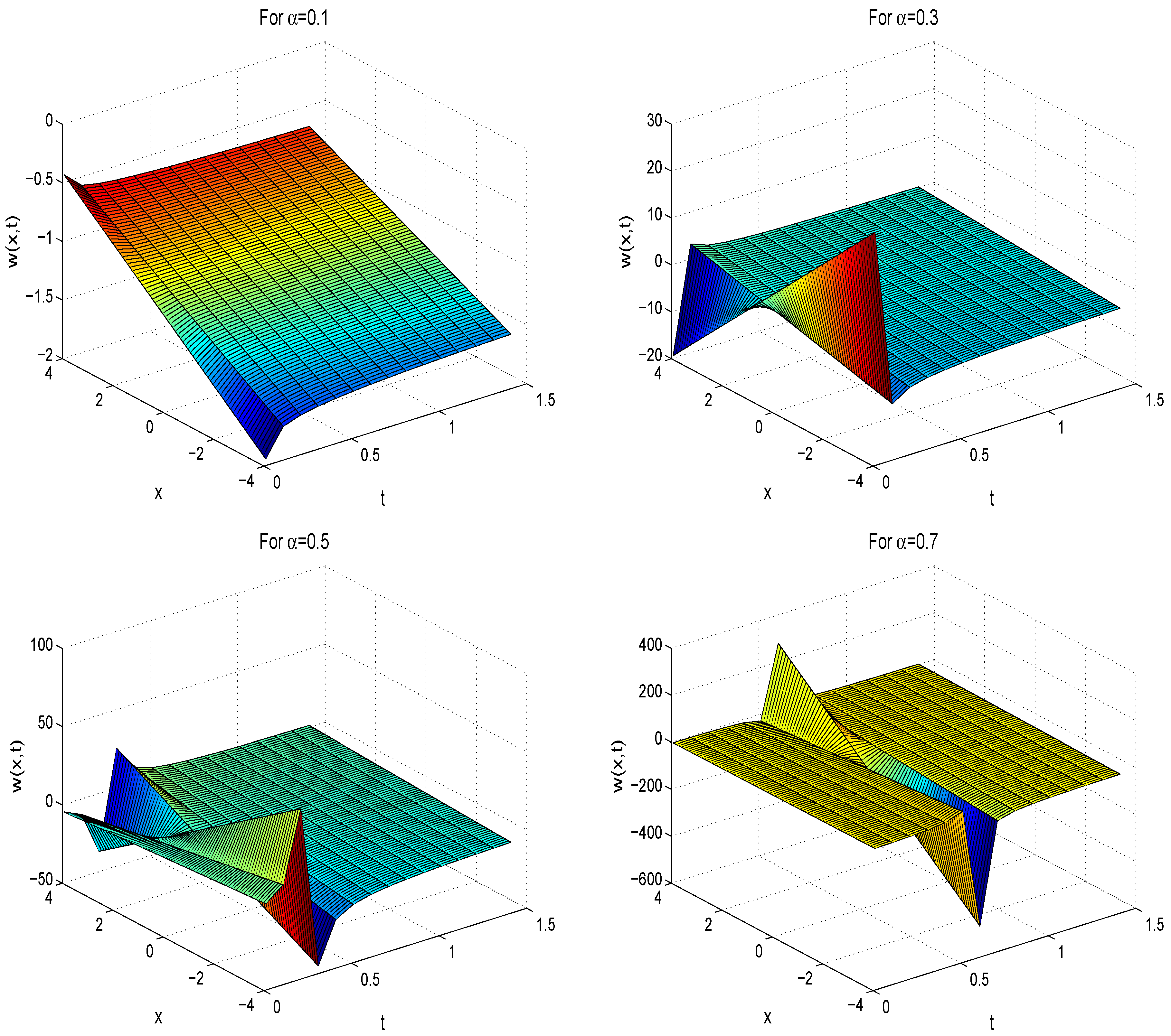
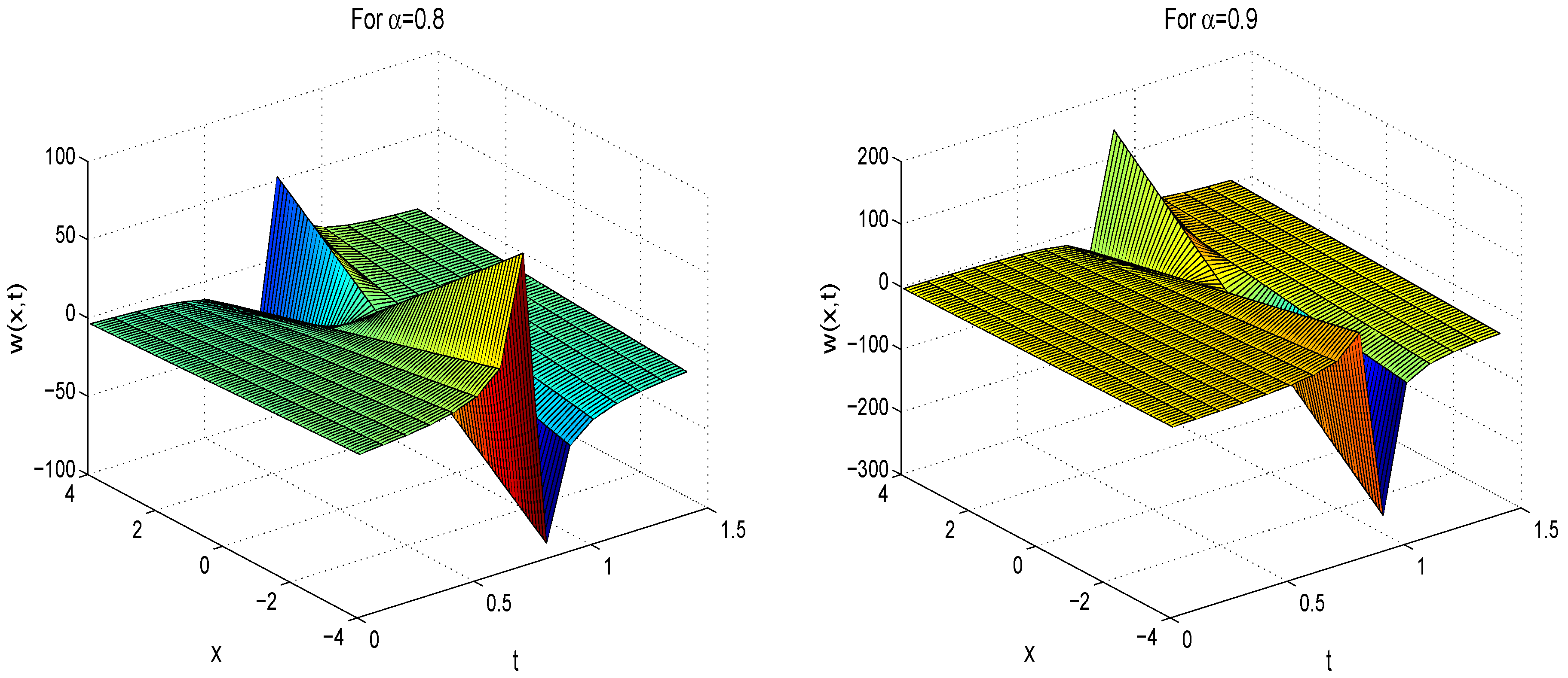
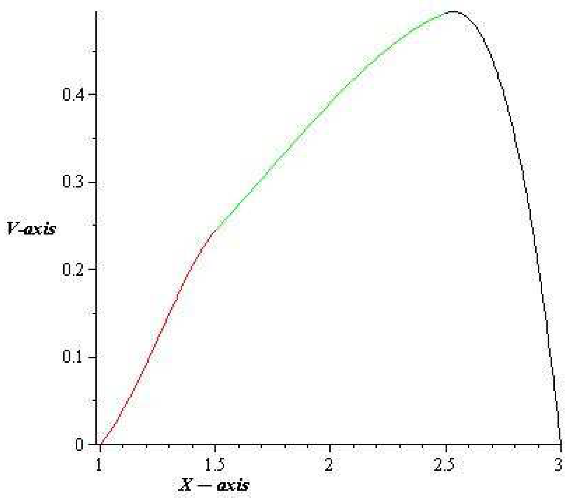
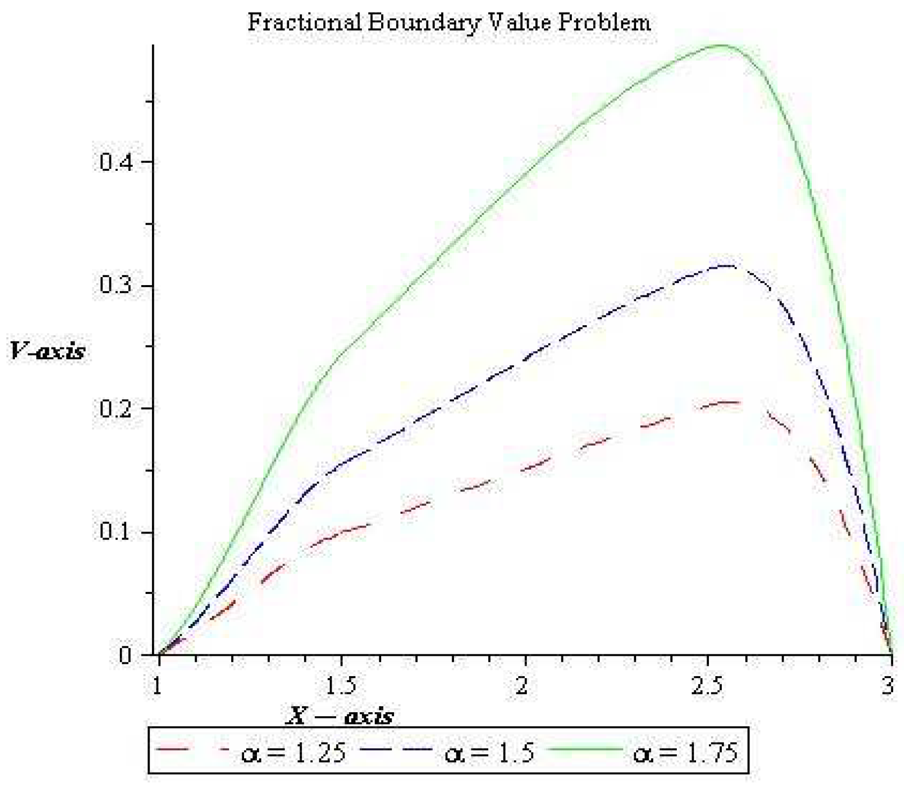
Discussion
In this section, results obtained by HPM are discussed. Analytical series solution of space-time FBP equation is given in Equation (
9). In
Figure 1, a solution is presented for different values of
.
Figure 1 shows a big difference in smaller and larger values of
. For larger values of
,
attains height and for values closer to 0, height of
reduces. In
Figure 2, results are presented for
and
, respectively. Exact solution of FBP model for
is given in Equation (
12). Equation (
12) shows discontinuity at
which is clearly depicted in
Figure 2. As value of
approaches to 1, the shock is produced in the vicinity of
.
5. Test Problem 2
Consider the fractional second-order obstacle BVP:
with boundary conditions
In order to apply HPM, we construct homotopy in three different domains:
Here
p is parameter that lies between 0 and 1. The solution
is given as follows:
Now, substitute Equation (
3) in Equation (
2), and comparing the coefficients of similar powers of
p, we get
Now, the fractional integral operator
with comfortable derivative definition is applied on both sides of Equation (
5), we get
Case II:
or
Now, substitute Equation (
3) in Equation (
7), and comparing the coefficients of similar powers of
p, we get
Now, the fractional integral operator
with comfortable derivative definition is applied on both sides of Equation (
8), we get
Case III:
In this case, the constructed homotopy will be same as in Case I. After substituting Equation (
3) in Equation (
2), we get
We calculate the results by taking and .
Now by applying the continuity conditions at
and
and BCs, we get a system of six nonlinear equations. By using Newton’s method for nonlinear system, we obtain the values of constants:
By substituting values of constants from Equation (
12) into Equation (
11), we get the analytical solution of system of second-order fractional BVPs subject to obstacle problem given in Equation (
1).
In similar manners, we can find the solution of problem mentioned in Equation (
1) for
and
.
2. For
We get the following analytical solution of system given in Equation (
1) for
.
3. For
We obtain the following analytical solution of the considered problem given in Equation (
1) for
is as follows:
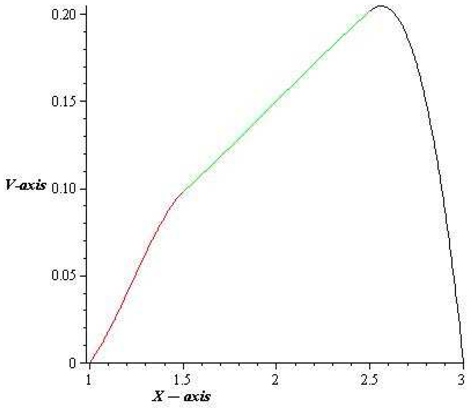
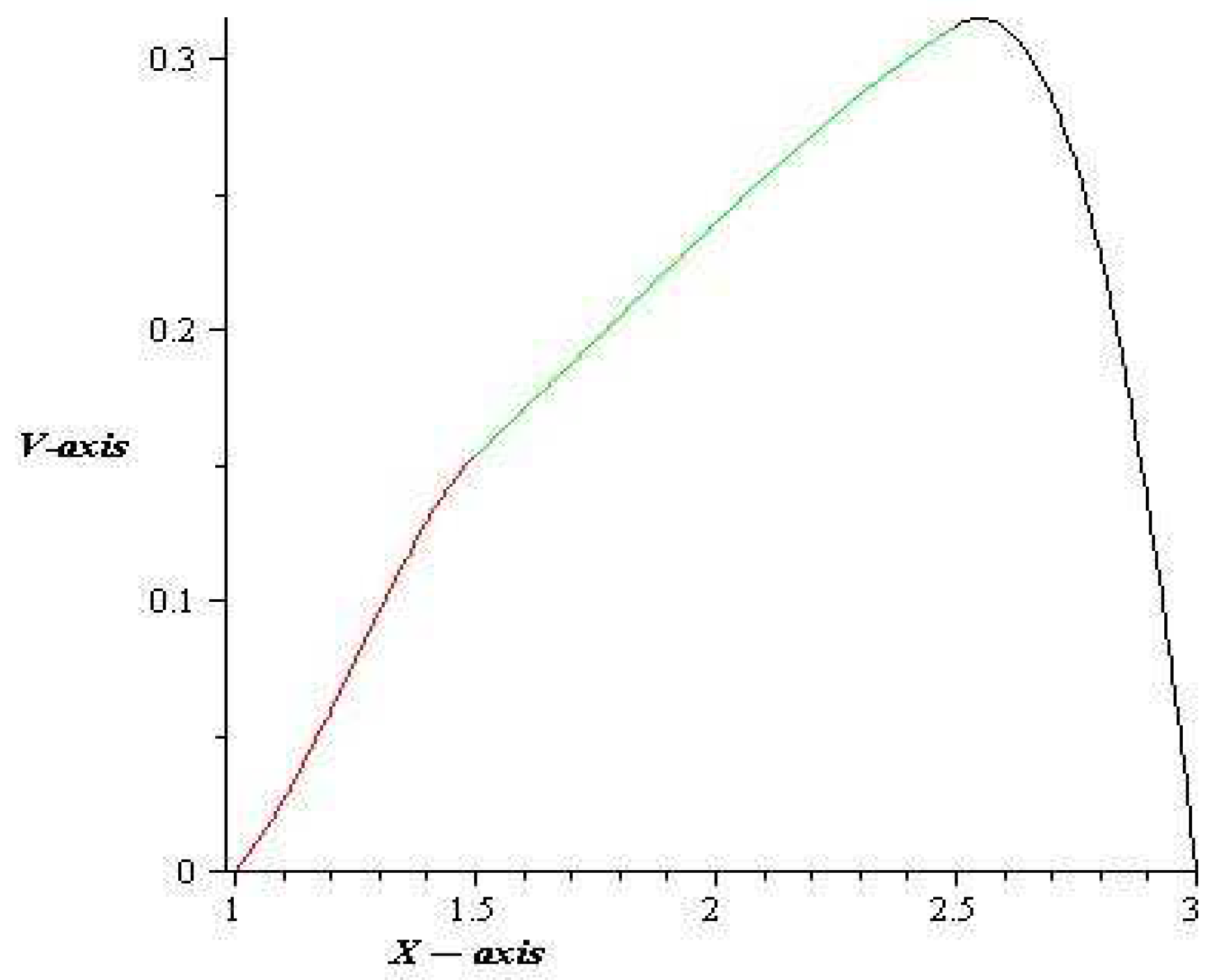
Discussion
Figure 3,
Figure 4 and
Figure 5 present the solution of obstacle problem for different values of
,
,
, respectively.
Figure 6 shows the comparison between different values of
. In
Figure 6, obstacle achieves more height for larger values of
and vice versa.
6. Conclusions
The analysis of HPM for the solution of FPDEs was given. A unified convergence theorem was proved and results were validated for the solution of FBP equation. The method to solve FPDEs was presented, while the same partial differential equation with ordinary derivative i.e., for fails to exist. This study demonstrated the importance of fractional derivative and the technique of dealing with these types of PDEs where solution of some ordinary PDEs does not exist. Moreover, HPM was applied to solve complex obstacle BVP. The suggested method can be applied to find solutions of other PDEs (both linear and nonlinear) of fractional order. The present study can be useful to analyze other traditional analytical techniques, such as Adomian Decomposition Method and Homotopy Analysis Method, to solve nonlinear differential equation of non- integer order. Furthermore, the present work may be extended to solve practical fractional models, for example wireless networks and nonlinear obstacle problems.
Author Contributions
Conceptualization, S.J; Methodology, S.J. and A.W; Software, S.J. and A.W; Validation, D.B and H.A.; Writing—original draft preparation, S.J, M.S.K and H.A.; Writing—review and editing, D.B.; Visualization, M.S.K; Supervision, D.B.
Funding
This research received no external funding.
Acknowledgments
The authors gratefully acknowledge Muhammad Asif Javed for helping in grammatical and stylistic editing of the article. The authors are thankful to Aqsa Mumtaz for helping in applying the code in Maple software.
Conflicts of Interest
The authors declare no conflict of interest.
Abbreviations
The following abbreviations are used in this manuscript:
| conformable derivative |
| conformable integral |
| HPM | homotopy perturbation method |
| FPDEs | fractional partial differential equations |
| BVP | boundary value problem |
| FDEs | fractional differential equations |
| PDEs | partial differential equations |
References
- Aslan, E.C.; Inc, M.; Al Qurashi, M.M.; Baleanu, D. On numerical solutions of time-fraction generalized Hirota Satsuma coupled KdV equation. J. Nonlinear Sci. Appl. 2017, 2, 724–733. [Google Scholar] [CrossRef]
- Garrappa, R. Numerical Solution of Fractional Differential Equations: A Survey and a Software Tutorial. Mathematics 2018, 6, 16. [Google Scholar] [CrossRef]
- Jafarian, A.; Mokhtarpour, M.; Baleanu, D. Artificial neural network approach for a class of fractional ordinary differential equation. Neural Comput. Appl. 2017, 4, 765–773. [Google Scholar] [CrossRef]
- Mainardi, F. Fractional Calculus: Theory and Applications. Mathematics 2018, 6, 145. [Google Scholar] [CrossRef]
- Miller, K.S.; Ross, B. An Introdution to the Fractional Calculus and Fractional Differential Equations; J. Willey & Sons: New York, NY, USA, 1993. [Google Scholar]
- Podlubny, I. Fractional Differential Equations; Academic Press: San Diego, CA, USA, 1999. [Google Scholar]
- Zappone, A.; Jorswieck, E. Energy Efficiency in Wireless Networks via Fractional Programming Theory. Found. Trends Commun. Inf. Theory 2014, 11, 185–396. [Google Scholar] [CrossRef]
- Apostolopoulos, P.A.; Tsiropoulou, E.E.; Papavassiliou, S. Demand Response Management in Smart Grid Networks: A Two-Stage Game-Theoretic Learning-Based Approach. Mob. Netw. Appl. 2018, 1–14. [Google Scholar] [CrossRef]
- Pan, I.; Das, S. Kriging Based Surrogate Modeling for Fractional Order Control of Microgrids. IEEE Trans. Smart Grid 2015, 6, 36–44. [Google Scholar] [CrossRef] [Green Version]
- Jindal, N.; Weber, S.; Andrews, J.G. Fractional power control for decentralized wireless networks. IEEE Trans. Wirel. Commun. 2008, 7, 5482–5492. [Google Scholar] [CrossRef] [Green Version]
- Thabet, H.; Kendre, S.; Chalishajar, D. New Analytical Technique for Solving a System of Nonlinear Fractional Partial Differential Equations. Mathematics 2017, 5, 47. [Google Scholar] [CrossRef]
- Abel, N.H. Solutions de quelques problems a l’aide d’integrales definies. Werk 1823, 1, 10–14. [Google Scholar]
- Caputo, M. Linera Models of Dissipation Whose q is Almost Frequency Independent. Ann. Geophys. 1966, 19, 383–393. [Google Scholar]
- Euler, L. On transcendental progression that is, those whose general terms cannot be given algebraically. Acad. Sci. Imperials Petropolitanae 1738, 1, 38–57. [Google Scholar]
- Fourier, J. Theorie Analytique de la Chaleur; Gauthier-Villars: Paris, France, 1888. [Google Scholar]
- Laplace, P.S. Theorie Analytique de Probabilities; Courcier: Paris, France, 1812. [Google Scholar]
- Liouville, J. Memory on a few questions of geometry and mechanics, and on a new kind of calculation to solve these questions (In France). J. de l’Ecole R. Polytechn 1832, 131–169. [Google Scholar]
- Ross, B. The development of fractional calculus 1695–1900. Hist. Math. 1974, 4, 75–89. [Google Scholar] [CrossRef]
- Oldham, K.B.; Spanier, J. The Fractional Calculus; Acad. Press: New York, NY, USA, 1974. [Google Scholar]
- He, J.H. Homotopy perturbation technique. Comput. Methods Appl. Mech. Eng. 1999, 178, 257–262. [Google Scholar] [CrossRef]
- He, J.H. Perturbation Methods: Basic and Beyond; Elsevier: Amsterdam, The Netherlands, 2006. [Google Scholar]
- Elsaid, A.; Hammad, D. A reliable treatment of homotopy perturbation method for the Sine-Gordon equation of arbitrary (fractional) order. J. Fract. Calc. Appl. 2012, 2, 1–8. [Google Scholar]
- AEl-Sayed, M.; Elsaid, A.; El-Kalla, I.L.; Hammad, D. A homotopy perturbation technique for solving partial differential equations of fractional order in finite domains. Appl. Math. Comput. 2012, 218, 8329–8340. [Google Scholar] [CrossRef]
- He, J.H. Application of homotopy perturbation method to nonlinear wave equations. Chaos Solitons Fract. 2005, 26, 695–700. [Google Scholar] [CrossRef]
- Momani, S.; Yildirim, A. Analytical approximate solutions of the fractional convection-diffusion equation with nonlinear source term by He’s homotopy perturbation method. Int. J. Comput. Math. 2010, 87, 1057–1065. [Google Scholar] [CrossRef]
- Momani, S.; Odibat, Z. Homotopy perturbation method for nonlinear partial differential equation of fractional order. Phys. Lett. A 2007, 365, 345–350. [Google Scholar] [CrossRef]
- Wang, Q. Homotopy perturbation method for fractional Kdv-Burgers Equation. Chaos Solitons Fract. 2008, 35, 843–850. [Google Scholar] [CrossRef]
- Fellner, K.; Schmeiser, C. Burgers-Poisson: A nonlinear dispersive Model equation. SIAM J. Appl. Math. 2004, 64, 1509–1525. [Google Scholar]
- Tian, L.; Gao, Y. The global attractor of the viscous Fornberg–Whitham equation. Nonlinear Anal. 2009, 71, 5176–5186. [Google Scholar] [CrossRef]
- Abidi, F.; Omrani, K. The homotopy analysis method for solving the Fornberg–Whitham equation and comparison with Adomian’s decomposition method. Comput. Math. Appl. 2010, 59, 2743–2750. [Google Scholar] [CrossRef] [Green Version]
- Rodrigues, J.F. Obstacle Problems in Mathematical Physics; Elsevier Science Publishers: Amsterdam, The Netherlands, 1987. [Google Scholar]
- Çenesiz, Y.; Baleanu, D.; Kurt, A.; Tasbozan, O. New exact solutions of Burgers’ type equations with conformable derivative. Waves Random Complex Media 2017, 1, 103–116. [Google Scholar] [CrossRef]
- Khalil, R.; al Horani, M.; Yousef, A.; Sababheh, M. A new definition of fractional derivative. J. Comput. Appl. Math. 2014, 264, 65–70. [Google Scholar] [CrossRef]
- Biazar, J.; Ghazvini, H. Convergence of the homotopy perturbation method for partial differential equations. Nonlinear Anal. Real World Appl. 2009, 10, 2633–2640. [Google Scholar] [CrossRef]
- Banach, S. Sur les opérations dans les ensembles abstraits et leur application aux équations intégrales. Fund. Math. 1922, 10, 133–181. [Google Scholar] [CrossRef]
- Gupta, P.K.; Singh, M. Homotopy perturbation method for fractional Fornberg-Whitham equation. Comput. Math. Appl. 2011, 61, 250–254. [Google Scholar] [CrossRef]
- Zeng, C.; Yang, Q.; Zhang, B. Homotopy perturbation method for fractional-order Burgers-Poisson equation. arXiv, 2010; arXiv:1003.1828. [Google Scholar]
© 2019 by the authors. Licensee MDPI, Basel, Switzerland. This article is an open access article distributed under the terms and conditions of the Creative Commons Attribution (CC BY) license (http://creativecommons.org/licenses/by/4.0/).


