Explicit Solutions and Bifurcations for a System of Rational Difference Equations

Abstract

In this paper, we consider the explicit solution of the following system of nonlinear rational difference equations: $x_{n+1}=x_{n-1}/\left(x_{n-1}+r\right)$, $y_{n+1}=x_{n-1}{y}_n/\left(x_{n-1}{y}_n+r\right)$, with initial conditions $x_{-1}$, $x_0$ and $y_0$, which are arbitrary positive real numbers. By doing this, we encounter the hypergeometric function. We also investigate global dynamics of this system. The global dynamics of this system consists of two kind of bifurcations.

1. Introduction and Preliminaries

Difference equations play an important role in many disciplines including biology, ecology, physics, economics, and many more [1,2]. These equations appear naturally as discrete analogs of differential equations, and as numerical solutions of differential and delay differential equations. Although most of these equations have a simple form, it is extremely difficult to understand their local and global dynamics including the existence, the boundedness, the asymptotic local stability, and the periodicity of solutions. Recently, there has been an increased interest in the quantitative as well as qualitative analysis of difference equations. One type of such difference equations that have been considered and examined by researchers is the nonlinear rational difference equations [3,4,5]. The study of rational difference equations is of crucial importance, since we know so little about such equations.

Amleh et al. [6] considered the nonlinear difference equation $x_n=\alpha +x_{n-1}/x_n$, where the parameter $\alpha$ and the initial condition $x_0$ are arbitrary positive real number. They proved that, if $x_n$ is a nontrivial solution of the equation so that there is a $n_0$ such that $x_n\ge \alpha +1$ for $n\ge n_0$, then $x_n$ is monotonically convergent to zero. In [7], Cinar studied the periodicity and the positive solution of the rational difference equations system $x_{n+1}=1/y_n$, $y_{n+1}=y_n/(x_{n-1}{y}_{n-1})$. The global character of solutions of the the system $x_{n+1}=(h+x_n)/(a+y_n)$, $y_{n+1}=y_n/(b+x_n)$ with positive parameters is studied in [8]. Kurbanli et al. [9] investigated the positive solutions of the system of difference equations $x_{n+1}=x_{n-1}/(y_n{x}_{n-1}+1)$, $y_{n+1}=y_{n-1}/(x_n{y}_{n-1}+1)$. Yalcinkaya et al. [10] investigated the sufficient conditions for the global asymptotic stability of the following system $x_{n+1}=(x_n+y_{n-1})/(x_n{y}_{n-1}-1)$, $y_{n+1}=(y_n+x_{n-1}/(y_n{x}_{n-1}-1)$. Khyat [11] studied many types of bifurcations for systems of several systems of rational difference equations. Many papers deal with the difference equations system. We refer in particular to [11,12,13,14] where further references can be found.

Our goal in this paper is to investigate the explicit solution of the following system of nonlinear rational difference equations systems

$$\left(\begin{array}{c}{x}_{n+1}\\ y_{n+1}\end{array}\right)=\left(\begin{array}{c}\frac{x_{n-1}}{x_{n-1}+r}\\ \frac{x_{n-1}{y}_n}{x_{n-1}{y}_n+r}\end{array}\right)$$

(1)

where the parameter r and the initial conditions $x_{-1}$, $x_0$, $y_0$ are arbitrary positive real numbers. Moreover, we investigate the global dynamics that occur in Equation (1). We show that the system in Equation (1) can have three fixed points and, using linear stability analysis, all transitions are determined under which fixed points lose stability. The bifurcations that occur in Equation (1) are numerically studied with a one-parameter bifurcation analysis.

2. The General Solution

Assume that the initial values are $x_{-1}=b$, $x_0=a$, $y_0=c$, then substituting $n=0,1,2,3,\dots$ into Equation (1) gives the following expressions for $x_n$ and $y_n$:

$$x_n=\left\{\begin{array}{ccc}\frac{a}{W_k(a)}& \mathrm{if}& n=2k\hfill \\ \frac{b}{W_{k+1}(b)}& \mathrm{if}& n=2k+1\hfill \end{array}\right.,y_n=\left\{\begin{array}{ccc}\frac{{(ab)}^{k}c}{P_n}& \mathrm{if}& n=2k\hfill \\ \frac{{(ab)}^{k}bc}{P_n}& \mathrm{if}& n=2k+1\hfill \end{array}\right.$$

(2)

where $k=0,1,2,3,\dots$, $W_0(a)=1$, $W_k(a)=a+r{W}_{k-1}(a)$, and the $P_i$ represents the denominator for $y_i$ after ith iteration where $P_0=1$ and $P_1=bc+r$. Formula for the sequence $\left\{P_i\right\}$ is a function of initial conditions. We use the above expressions to find

$$y_{2k+2}=\frac{{(ab)}^{k+1}c}{P_{2k+2}},y_{2k+3}=\frac{{(ab)}^{k+1}bc}{P_{2k+3}}$$

(3)

On the other hand, by using Equations (1) and (2), we obtain

$$y_{2k+2}=\frac{{(ab)}^{k+1}c}{{(ab)}^{k+1}c+r{P}_{2k+1}{W}_k(a)},y_{2k+3}=\frac{a^{k+1}{b}^{k+2}c}{{(ab)}^{k+1}bc+r{P}_{2k+2}{W}_{k+1}(b)},$$

(4)

from

$$y_{2k+2}=\frac{x_{2k}{y}_{2k+1}}{x_{2k}{y}_{2k+1}+r},y_{2k+3}=\frac{x_{2k+1}{y}_{2k+2}}{x_{2k+1}{y}_{2k+2}+r}.$$

Comparing Equations (3) and (4), we find

$$P_{2k+2}={(ab)}^{k+1}c+r{P}_{2k+1}{W}_k(a),P_{2k+3}={(ab)}^{k+1}bc+r{P}_{2k+2}{W}_{k+1}(b).$$

This means that

$$\begin{array}{cc}\hfill P_0& =1,\hfill \\ \hfill P_1& =bc+r,\hfill \\ \hfill P_2& ={(ab)}^{1}c+r{W}_0(a)P_1,\hfill \\ \hfill P_3& ={(ab)}^{1}bc+{(ab)}^{1}cr{W}_1(b)+r^2{W}_0(a)W_1(b)P_1,\hfill \\ \hfill P_4& ={(ab)}^{2}c+{(ab)}^{1}bcr{W}_1(a)+{(ab)}^{1}c{r}^2{W}_1(a)W_1(b)+r^3{W}_0(a)W_1(a)W_1(b)P_1,\hfill \\ \hfill P_5& ={(ab)}^{2}bc+{(ab)}^{2}cr{W}_2(b)+{(ab)}^{1}bc{r}^2{W}_1(a)W_2(b)+{(ab)}^{1}c{r}^3{W}_1(a)W_1(b)W_2(b)\hfill \\ & +r^4{W}_0(a)W_1(a)W_1(b)W_2(b)P_1,\hfill \\ \hfill P_6& ={(ab)}^{3}c+{(ab)}^{2}bcr{W}_2(a)+{(ab)}^{2}c{r}^2{W}_2(a)W_2(b)+{(ab)}^{1}bc{r}^3{W}_1(a)W_2(a)W_2(b)\hfill \\ & +{(ab)}^{1}c{r}^4{W}_1(a)W_2(a)W_1(b)W_2(b)+r^5{W}_0(a)W_1(a)W_2(a)W_1(b)W_2(b)P_1,\hfill \\ & ⋮\hfill \end{array}$$

We summarize this in the following Lemma.

Lemma 1.

The following relations hold for $k\ge 0$.

$$\begin{array}{cc}\hfill P_{2k+2}& ={(ab)}^{k+1}c+{(ab)}^{k}bcr{Q}_k^k(a)+r^{2k+1}{Q}_1^k(a)Q_1^k(b)P_1+c{I}_k+c{J}_k,\hfill \\ \hfill P_{2k+3}& ={(ab)}^{k+1}bc+{(ab)}^{k+1}cr{Q}_{k+1}^{k+1}(b)+r^{2k+2}{Q}_1^k(a)Q_1^{k+1}(b)P_1+c{A}_k+c{B}_k,\hfill \end{array}$$

where

$$\begin{array}{c}{Q}_l^m(\xi )=\prod _{j=l}^m{W}_j(\xi ),\hfill \\ A_k=\sum _{n=1}^k{(ab)}^{k-n+1}b{r}^{2n}{Q}_{k-n+1}^k(a)Q_{k-n+2}^{k+1}(b),\hfill \\ B_k=\sum _{n=1}^k{(ab)}^{k-n+1}{r}^{2n+1}{Q}_{k-n+1}^k(a)Q_{k-n+1}^{k+1}(b),\hfill \\ I_k=\sum _{n=1}^k{(ab)}^{k-n+1}{r}^{2n}{Q}_{k-n+1}^k(a)Q_{k-n+1}^k(b),\hfill \\ J_k=\sum _{n=1}^{k-1}{(ab)}^{k-n}b{r}^{2n+1}{Q}_{k-n}^k(a)Q_{k-n+1}^k(b).\hfill \end{array}$$

Now, we consider a special case $x_{-1}=x_0=b$, $y_0=c$ and $r=1$ in order to simplify the computations. In this case, we are able to calculate the quantities in Lemma 1. By using the properties of gamma function, it is easy to prove the following Lemma.

Lemma 2.

For every positive real p and q, the following relation holds:

$$\prod _{j=m}^n(p+jq)=q^{n+1-m}\frac{\mathsf{\Gamma }(n+1+\frac{p}{q})}{\mathsf{\Gamma }(m+\frac{p}{q})}$$

According to Lemma 2, we write

$$\begin{array}{cc}\hfill Q_l^m(\xi )& ={\xi }^{m-l+1}\frac{\mathsf{\Gamma }(m+1+{\xi }^{-1})}{\mathsf{\Gamma }(l+{\xi }^{-1})},\hfill \\ \hfill I_k& =\sum _{n=1}^k{b}^{2k-2n+2}{b}^{2n}\frac{\mathsf{\Gamma }(k+1+b^{-1})}{\mathsf{\Gamma }(k-n+1+b^{-1})}\frac{\mathsf{\Gamma }(k+1+b^{-1})}{\mathsf{\Gamma }(k-n+1+b^{-1})}\hfill \\ & =b^{2k+2}\mathsf{\Gamma }{(k+1+b^{-1})}^2\sum _{n=1}^k\frac{1}{\mathsf{\Gamma }{(k-n+1+b^{-1})}^2}\hfill \\ \hfill J_k& =\sum _{n=1}^{k-1}{b}^{2k-2n}b{b}^{2n+1}\frac{\mathsf{\Gamma }(k+1+b^{-1})}{\mathsf{\Gamma }(k-n+b^{-1})}\frac{\mathsf{\Gamma }(k+1+b^{-1})}{\mathsf{\Gamma }(k-n+1+b^{-1})}\hfill \\ & =b^{2k+2}\mathsf{\Gamma }{(k+1+b^{-1})}^2\sum _{n=1}^{k-1}\frac{1}{\mathsf{\Gamma }(k-n+b^{-1})\mathsf{\Gamma }(k-n+1+b^{-1})},\hfill \end{array}$$

Similarly, we write

$$\begin{array}{cc}\hfill A_k& =b^{2k+3}\mathsf{\Gamma }(k+1+b^{-1})\mathsf{\Gamma }(k+2+b^{-1})\sum _{n=1}^k\frac{1}{\mathsf{\Gamma }(k-n+1+b^{-1})\mathsf{\Gamma }(k-n+2+b^{-1})},\hfill \\ \hfill B_k& =b^{2k+3}\mathsf{\Gamma }(k+1+b^{-1})\mathsf{\Gamma }(k+2+b^{-1})\sum _{n=1}^k\frac{1}{\mathsf{\Gamma }{(k-n+1+b^{-1})}^2}.\hfill \end{array}$$

and

$$\begin{array}{cc}\hfill \sum _{j=1}^n\frac{1}{\mathsf{\Gamma }(j+b^{-1})\mathsf{\Gamma }(j+1+b^{-1})}& =\frac{F_1^2(1;1+b^{-1},2+b^{-1};1)}{\mathsf{\Gamma }(1+b^{-1})\mathsf{\Gamma }(2+b^{-1})}-\frac{F_1^2(1;n+1+b^{-1},n+2+b^{-1};1)}{\mathsf{\Gamma }(n+1+b^{-1})\mathsf{\Gamma }(n+2+b^{-1})},\hfill \\ \hfill \sum _{j=1}^n\frac{1}{\mathsf{\Gamma }{(j+b^{-1})}^2}& =\frac{F_1^2(1;1+b^{-1},1+b^{-1};1)}{\mathsf{\Gamma }{(1+b^{-1})}^2}-\frac{F_1^2(1;n+1+b^{-1},n+1+b^{-1};1)}{\mathsf{\Gamma }{(n+1+b^{-1})}^2}.\hfill \end{array}$$

where $F_1^2$ is the hypergeometric function. We introduce the notation

$$D(n,m)=\frac{F_1^2(m-n+1;1+b^{-1},m-n+1+b^{-1};1)}{\mathsf{\Gamma }(m-n+1+b^{-1})\mathsf{\Gamma }(m-n+1+b^{-1})}-\frac{F_1^2(1;n+1+b^{-1},m+1+b^{-1};1)}{\mathsf{\Gamma }(n+1+b^{-1})\mathsf{\Gamma }(m+1+b^{-1})}$$

Hence, we conclude

$$\begin{array}{cc}\hfill A_k+B_k& =b^{2k+3}\mathsf{\Gamma }(k+1+b^{-1})\mathsf{\Gamma }(k+2+b^{-1})(D(k,k+1)+D(k,k)),\hfill \\ \hfill I_k+J_k& =b^{2k+2}\mathsf{\Gamma }(k+1+b^{-1})\mathsf{\Gamma }(k+1+b^{-1})(D(k,k)+D(k-1,k)),\hfill \end{array}$$

We use the notation $v(l)$ as the greatest integer function. We reach the following proposition.

Proposition 1.

For $x_{-1}=x_0=b$, $y_0=c$, $r=1$ and $n\ge 4$, the general form of the solution of Equation (1) is

$$\left(\begin{array}{c}{x}_n\\ y_n\end{array}\right)=\left(\begin{array}{c}\frac{b}{bv\left(\frac{n+1}{2}\right)+1}\\ \frac{b^{n}c\mathsf{\Gamma }{(\frac{n}{2}+b^{-1})}^{-1}\mathsf{\Gamma }{(v\left(\frac{n+1}{2}\right)+b^{-1})}^{-1}}{b^{n}c\left[D(v\left(\frac{n+1}{2}\right)-1,v\left(\frac{n+1}{2}\right))+D\left(v\left(\frac{n}{2}\right),v\left(\frac{n}{2}\right)\right)\right]+b^{n-2}{P}_1\mathsf{\Gamma }{(1+b^{-1})}^{-2}}\end{array}\right)$$

Proof. 

By using Lemma 1, we have

$$P_{2k+2}=c({(b^2)}^{k+1}+{(b^2)}^{k}b{Q}_k^k(b)+I_k+J_k)+Q_1^k(b)Q_1^k(b)P_1,$$

on the other hand, by using the expressions for $I_k+J_k$ and $Q_l^m$, we obtain

$$\begin{array}{cc}\hfill b^{2k+2}& +b^{2k+1}{Q}_k^k(b)+I_k+J_k\hfill \\ & =b^{2k+2}(1+\frac{\mathsf{\Gamma }(k+1+b^{-1})}{\mathsf{\Gamma }(k+b^{-1})}+\mathsf{\Gamma }{(k+1+b^{-1})}^2(D(k,k)+D(k-1,k)))\hfill \\ & =b^{2k+2}\mathsf{\Gamma }{(k+1+b^{-1})}^2(\frac{1}{\mathsf{\Gamma }{(k+1+b^{-1})}^2}+\frac{1}{\mathsf{\Gamma }(k+b^{-1})\mathsf{\Gamma }(k+1+b^{-1})}+D(k,k)+D(k-1,k))\hfill \\ & =b^{2k+2}\mathsf{\Gamma }{(k+1+b^{-1})}^2(D(k+1,k+1)+D(k,k+1)),\hfill \end{array}$$

and

$$Q_1^k(b)Q_1^k(b)P_1=b^{2k}{P}_1\frac{\mathsf{\Gamma }{(k+1+b^{-1})}^2}{\mathsf{\Gamma }{(1+b^{-1})}^2}$$

Now, we obtain

$$P_{2k+2}=\mathsf{\Gamma }{(k+1+b^{-1})}^2(b^{2k+2}c(D(k+1,k+1)+D(k,k+1))+\frac{b^{2k}{P}_1}{\mathsf{\Gamma }{(1+b^{-1})}^2})$$

(5)

Similarly, we obtain

$$P_{2k+3}=c{b}^{2k+2}U+Q_1^k(b)Q_1^{k+1}(b)P_1,$$

where

$$\begin{array}{cc}\hfill U& =b+Q(k+1,k+1,b)+b\mathsf{\Gamma }(k+1+b^{-1})\mathsf{\Gamma }(k+2+b^{-1})(D(k,k+1)+D(k,k))\hfill \\ & =b(1+\frac{\mathsf{\Gamma }(k+2+b^{-1})}{\mathsf{\Gamma }(k+1+b^{-1})}+\mathsf{\Gamma }(k+1+b^{-1})\mathsf{\Gamma }(k+2+b^{-1})(D(k,k+1)+D(k,k)))\hfill \\ & =b\mathsf{\Gamma }(k+1+b^{-1})\mathsf{\Gamma }(k+2+b^{-1}(D(k+1,k+2)+D(k+1,k+1)),\hfill \end{array}$$

and

$$Q_1^k(b)Q_1^{k+1}(b)P_1=b^{2k+1}{P}_1\frac{\mathsf{\Gamma }(k+1+b^{-1})\mathsf{\Gamma }(k+2+b^{-1})}{\mathsf{\Gamma }{(1+b^{-1})}^2}$$

Hence,

$$\begin{array}{cc}\hfill P_{2k+3}& =\mathsf{\Gamma }(k+1+b^{-1})\mathsf{\Gamma }(k+2+b^{-1})\left(b^{2k+3}c(D(k+1,k+2)+D(k+1,k+1))\right.\hfill \\ & \left.+\frac{b^{2k+1}{P}_1}{\mathsf{\Gamma }{(1+b^{-1})}^2}\right).\hfill \end{array}$$

(6)

From Equations (5) and (6), we are done since

$$\begin{array}{cc}\hfill v\left(\frac{2k+3}{2}\right)& =k+1,v\left(\frac{2k+3+1}{2}\right)=k+2,\hfill \\ \hfill v\left(\frac{2k+2}{2}\right)& =k+1,v\left(\frac{2k+2+1}{2}\right)=k+1.\hfill \end{array}$$

 □

Example 1.

If we take $a=b=\frac{1}{3}$, $c=3$ and $r=1$, then, by direct computations, we obtain

$$\begin{array}{ccc}\left(\begin{array}{c}{x}_1\\ y_1\end{array}\right)=\left(\begin{array}{c}\frac{1}{4}\\ \frac{1}{2}\end{array}\right),\hfill & \left(\begin{array}{c}{x}_2\\ y_2\end{array}\right)=\left(\begin{array}{c}\frac{1}{4}\\ \frac{1}{7}\end{array}\right),\hfill & \left(\begin{array}{c}{x}_3\\ y_3\end{array}\right)=\left(\begin{array}{c}\frac{1}{5}\\ \frac{1}{29}\end{array}\right),\hfill \\ \left(\begin{array}{c}{x}_4\\ y_4\end{array}\right)=\left(\begin{array}{c}\frac{1}{5}\\ \frac{1}{117}\end{array}\right),\hfill & \left(\begin{array}{c}{x}_5\\ y_5\end{array}\right)=\left(\begin{array}{c}\frac{1}{6}\\ \frac{1}{586}\end{array}\right),\hfill & \left(\begin{array}{c}{x}_6\\ y_6\end{array}\right)=\left(\begin{array}{c}\frac{1}{6}\\ \frac{1}{2931}\end{array}\right).\hfill \end{array}$$

It is easy to see that $P_1=2$. Now, we have

$$\begin{array}{cc}\hfill D(1,2)& =\frac{F_1^2(1;1+3,2+3;1)}{\mathsf{\Gamma }(1+3)\mathsf{\Gamma }(2+3)}-\frac{F_1^2(1;1+1+3,2+1+3;1)}{\mathsf{\Gamma }(1+1+3)\mathsf{\Gamma }(1+2+3)}=\frac{1}{144},\hfill \\ \hfill D(2,2)& =\frac{17}{576},\hfill \\ \hfill D(2,3)& =\frac{7}{960},\hfill \\ \hfill D(3,3)& =\frac{71}{2400},\hfill \end{array}$$

$$\begin{array}{cc}\hfill y_4& =\frac{3^{-3}{\mathsf{\Gamma }((2+3)}^{-1}\mathsf{\Gamma }{(2+3)}^{-1}}{3^{-3}(D(1,2)+D(2,2))+3^{-2}{P}_1\mathsf{\Gamma }{(1+3)}^{-2}}=\frac{\frac{1}{15552}}{\frac{1}{27}(\frac{4}{576}+\frac{17}{576})+\frac{2}{324}}\hfill \\ & =\frac{1}{21+96}=\frac{1}{117},\hfill \\ \hfill y_5& =\frac{3^{-4}\mathsf{\Gamma }{(2+3)}^{-1}\mathsf{\Gamma }{(3+3)}^{-1}}{3^{-4}(D(2,3)+D(2,2))+3^{-3}{P}_1\mathsf{\Gamma }{(1+3)}^{-2}}=\frac{\frac{1}{233280}}{\frac{1}{81}(\frac{7}{960}+\frac{17}{576})+\frac{2}{972}}\hfill \\ & =\frac{1}{233280(\frac{1}{81}\frac{53}{1440}+\frac{1}{486})}=\frac{1}{233280(\frac{53}{116640}+\frac{240}{116640})}=\frac{1}{2(293)}=\frac{1}{586},\hfill \\ \hfill y_6& =\frac{3^{-5}{\mathsf{\Gamma }((3+3)}^{-1}\mathsf{\Gamma }{(3+3)}^{-1}}{3^{-5}(D(2,3)+D(3,3))+3^{-4}{P}_1\mathsf{\Gamma }{(1+3)}^{-2}}=\frac{\frac{1}{3499200}}{\frac{1}{243}(\frac{7}{960}+\frac{71}{2400})+\frac{2}{2916}}\hfill \\ & =\frac{1}{14400\frac{59}{1600}+\frac{3499200}{1458}}=\frac{1}{531+2400}=\frac{1}{2931}\hfill \end{array}$$

3. Bifurcation Analysis

Consider the nested system in Equation (1). We introduce a new variable z, which is defined as $z_n=x_{n-1}$ ($z_{n+1}=x_n$), and then the system in Equation (1) can be expressed by the following three-dimensional system of difference equations:

$$\left(\begin{array}{c}{x}_{n+1}\\ y_{n+1}\\ z_{n+1}\end{array}\right)=\left(\begin{array}{c}\frac{z_n}{z_n+r}\\ \frac{z_n{y}_n}{z_n{y}_n+r}\\ x_n\end{array}\right)$$

or in vector form as

$$X_{n+1}=F(X_n,r),F:{\mathbb{R}}^3\times \mathbb{R}\to {\mathbb{R}}^3,$$

(7)

where $n=0,1,2,\dots$, $X_n=(x_n,y_n,z_n)$, $F=\left(\frac{z_n}{z_n+r},\frac{z_n{y}_n}{z_n{y}_n+r},x_n\right)$, $r\in \mathbb{R}$, and the initial point $X_0$ is positive. The fixed points of Equation (7) can be found by solving the system $F(X^{\ast },r)-X^{\ast }=0$. Thus, the system in Equation (7) can have three fixed points

$$X^i=\left(x^{(i)},y^{(i)},z^{(i)}\right)=\left\{\begin{array}{cc}(0,0,0),\hfill & i=1\hfill \\ (1-r,0,1-r),\hfill & i=2\hfill \\ \left(1-r,\frac{2r-1}{r-1},1-r\right),\hfill & i=3\hfill \end{array}\right.$$

It is known that a fixed point $X^{\ast }$ is (asymptotically) stable if all eigenvalues of the Jacobian matrix of Equation (7) evaluated at $X^{\ast }$ have absolute values less than one. Moreover, if at least one of the eigenvalues has absolute value greater than one, then the fixed point $X^{\ast }$ is unstable [5,15]. The Jacobian matrix of Equation (7) evaluated at the fixed point $X^i$,

$$A=\left(\begin{array}{ccc}0& 0& \frac{r}{{\left(z^{(i)}+r\right)}^2}\\ 0& \frac{r{z}^{(i)}}{{\left(z^{(i)}{y}^{(i)}+r\right)}^2}& \frac{r{y}^{(i)}}{{\left(z^{(i)}{y}^{(i)}+r\right)}^2}\\ 1& 0& 0\end{array}\right),$$

(8)

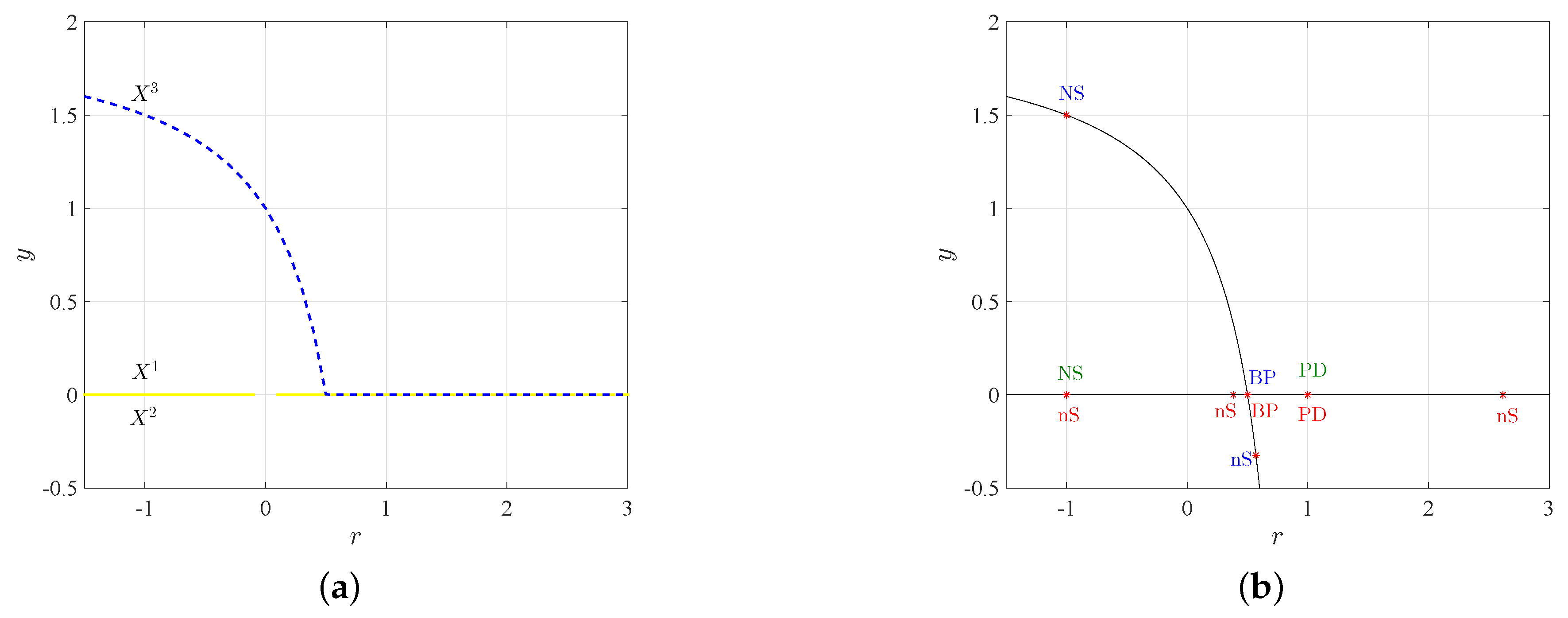
having the eigenvalues ${\mu }_1=\frac{r{z}^{(i)}}{{\left(z^{(i)}{y}^{(i)}+r\right)}^2},{\mu }_2=\frac{\sqrt{r}}{z^{(i)}+r},{\mu }_3=\frac{-\sqrt{r}}{z^{(i)}+r}$. Note that ${\mu }_3=-{\mu }_2$. The eigenvalues evaluated at the fixed points are summarized in

Table 1. The eigenvalues of the Jacobian matrix (Equation (8)).

Fixed Point	${\mathit{\mu }}_1$	${\mathit{\mu }}_2$	${\mathit{\mu }}_3$
$X^1$	0	$\frac{1}{\sqrt{r}}$	$-\frac{1}{\sqrt{r}}$
$X^2$	$\frac{1-r}{r}$	$\sqrt{r}$	$-\sqrt{r}$
$X^3$	$\frac{r}{1-r}$	$\sqrt{r}$	$-\sqrt{r}$

.

Proposition 2.

(i) 

The fixed point $X^1$ is stable for $r\in \mathbb{R}\backslash \left[-1,1\right]$ and unstable for $r\in \left(-1,1\right)$.

(ii) 

The fixed point $X^2$ is stable for $r\in \left(\frac{1}{2},1\right)$ and unstable for $r\in \mathbb{R}\backslash \left[\frac{1}{2},1\right]$.

(iii) 

The fixed point $X^3$ is stable for $r\in \left(-1,\frac{1}{2}\right)$ and unstable for $r\in \mathbb{R}\backslash \left[-1,\frac{1}{2}\right]$.

To study the type of bifurcations that occur in Equation (7), we need to look for parameter values for which Equation (7) has a fixed point with eigenvalues satisfying one of the bifurcation conditions (for more details, see [16,17]).

Proposition 3.

(i) 

The fixed points $X^1$ and $X^3$ lose stability via a 1:4 resonance Neimark–Sacker bifurcation point (NS) when $r=-1$ for which ${\mu }_{2,3}={\mathrm{e}}^{\pm i{\theta }_0}$, ${\theta }_0=\frac{\pi }{2}$.

(ii) 

The fixed points $X^2$ and $X^3$ lose stability via a branching point (BP) when $r=\frac{1}{2}$ for which ${\mu }_1=1$. The BP corresponds to the appearance where the curves of the fixed points $X^2$ and $X^3$ are intersect. This indicates the existence of other cycles with higher periods.

(iii) 

The fixed points $X^1$ and $X^2$ lose stability via a fold-flip period-doubling bifurcation point (PD) when $r=1$ for which ${\mu }_2=1$ and ${\mu }_3=-1$.

(iv) 

We can always find a neutral-saddle point (nS) points for which ${\mu }_i{\mu }_j=1$ along the curves of the fixed points

(a) 

$X^2$ when $r=\left\{-1,0.3819660112,2.618033989\right\}$.

(b) 

$X^3$ when $r=0.5698402917$.

The bifurcation diagram can be constructed by repeating the system in Equation (7), e.g., k-times, for different r and using the fixed points as initial point. Figure 1a plots the bifurcation diagram of the system in Equation (7) with $r\in [-1.5,3]$. For each r, the initial points were reset to

$$X_0=\left\{(\epsilon ,\epsilon ,\epsilon ),(1-r+\epsilon ,\epsilon ,1-r+\epsilon ),\left(1-r+\epsilon ,\frac{2r-1}{r-1}+\epsilon ,1-r+\epsilon \right)\right\},\epsilon ={10}^{-6}.$$

We performed ${10}^3$ iterations and then we discarded the first 500 iterations to avoid transit effects. This led to the bifurcation diagram in Figure 1a. This diagram is refined by a continuation method (by using the MATLAB package MatContM, see [18,19,20]). The result of the continuation method is shown in Figure 1b. In Figure 2a,b, we present the values for the eigenvalues during fixed point continuations using the three fixed points of Equation (7). This confirms the theoretical results derived above.

References

- Kelley, W.; Peterson, A. Difference Equations: An Introduction with Applications, 2nd ed.; Academic Press: New York, NY, USA, 2001. [Google Scholar]
- Mickens, R.E. Difference Equations: Theory, Applications and Advanced Topics, 3rd ed.; Chapman & Hall/CRC: Boca Raton, FL, USA, 2015. [Google Scholar]
- Kocic, V.L.; Ladas, G. Global Behavior of Nonlinear Difference Equations of Higher Order with Applications; Kluwer Academic: Dordrecht, The Netherlands, 1993. [Google Scholar]
- Kulenovic, M.R.S.; Ladas, G. Dynamics of Second Order Rational Difference Equations: With Open Problems and Conjectures; Chapman and Hall/CRC: Boca Raton, FL, USA, 2002. [Google Scholar]
- Kulenovic, M.R.S.; Merino, O. Discrete Dynamical Systems and Difference Equations with Mathematica; Chapman & Hall/CRC: London, UK, 2002. [Google Scholar]
- Amleh, A.M.; Grove, E.A.; Ladas, G.; Georgiou, D.A. On the Recursive Sequence xn+1 = α + xn−1/xn. J. Math. Anal. Appl. 1999, 2332, 790–798. [Google Scholar] [CrossRef]
- Cinar, C. On the positive solutions of the difference equation system xn+1 = 1/yn, yn+1 = yn/(xn−1yn−1). Appl. Math. Comput. 2004, 158, 303–305. [Google Scholar]
- Clark, C.A.; Kulenovic, M.R.S.; Selgrade, J.F. On a system of rational difference equations. J. Differ. Equ. Appl. 2005, 11, 565–580. [Google Scholar] [CrossRef]
- Kurbanli, A.S.; Cinar, C.; Yalcinkaya, I. On the behavior of positive solutions of the system of rational difference equations xn+1 = xn−1/(ynxn−1 + 1), yn+1 = yn−1/(xnyn−1 + 1). Math. Comput. Model. 2011, 53, 1261–1267. [Google Scholar] [CrossRef]
- Yalcinkaya, I.; Cinar, C.; Atalay, M. On the solutions of systems of difference equations. Adv. Differ. Equ. 2008, 2008, 143943. [Google Scholar] [CrossRef]
- Khyat, T. Bifurcations of Some Planar Discrete Dynamical Systems with Applications. Ph.D. Thesis, University of Rhode Island, Kingston, RI, USA, 2017. [Google Scholar]
- Kurbanli, A.S. On the behavior of solutions of the system of rational difference equations xn+1 = xn−1/(ynxn−1 − 1), yn+1 = yn−1/(xnyn−1 − 1), zn+1 = 1/(ynzn). Adv. Differ. Equ. 2011, 2011, 40. [Google Scholar] [CrossRef]
- Elsayed, E.M.; El-Metwally, H. On the solutions of some nonlinear systems of difference equations. Adv. Differ. Equ. 2013, 2013, 161. [Google Scholar] [CrossRef] [Green Version]
- El-Dessoky, M.M. On a solvable for some systems of rational difference equations. J. Nonlinear Sci. Appl. 2016, 9, 3744–3759. [Google Scholar] [CrossRef] [Green Version]
- Elaydi, S. Discrete Chaos; Chapman & Hall/CRC: London, UK, 2000. [Google Scholar]
- Arnold, V.I. Geometrical Methods in the Theory of Ordinary Differential Equations; Springer: New York, NY, USA; Heidelberg/Berlin, Germany, 1983. [Google Scholar]
- Kuznetsov, Y.A. Elements of Applied Bifurcation Theory, 3rd ed.; Springer: New York, NY, USA, 2004. [Google Scholar]
- Khoshsiar Ghaziani, R. Bifurcations of Maps: Numerical Algorithms and Applications. Ph.D. Thesis, Ghent University, Ghent, Belgium, 2008. [Google Scholar]
- Govaerts, W.; Kuznetsov, Y.A.; Khoshsiar Ghaziani, R.; Meijer, H.G.E. CL_MATCONTM: A Toolbox for Continuation and Bifurcation of Cycles of Maps; Report; Ghent University: Ghent, Belgium; Utrecht University: Utrecht, The Netherlands, 2008. [Google Scholar]
- Neirynck, N.; Al-Hdaibat, B.; Govaerts, W.; Kuznetsov, Y.A.; Meijer, H.G.E. Using MatContM in the study of a nonlinear map in economics. J. Phys. Conf. Ser. 2016, 692, 012013. [Google Scholar] [CrossRef] [Green Version]