All articles published by MDPI are made immediately available worldwide under an open access license. No special
permission is required to reuse all or part of the article published by MDPI, including figures and tables. For
articles published under an open access Creative Common CC BY license, any part of the article may be reused without
permission provided that the original article is clearly cited. For more information, please refer to
https://www.mdpi.com/openaccess.
Feature papers represent the most advanced research with significant potential for high impact in the field. A Feature
Paper should be a substantial original Article that involves several techniques or approaches, provides an outlook for
future research directions and describes possible research applications.
Feature papers are submitted upon individual invitation or recommendation by the scientific editors and must receive
positive feedback from the reviewers.
Editor’s Choice articles are based on recommendations by the scientific editors of MDPI journals from around the world.
Editors select a small number of articles recently published in the journal that they believe will be particularly
interesting to readers, or important in the respective research area. The aim is to provide a snapshot of some of the
most exciting work published in the various research areas of the journal.
Developed here are sixteenth-order simple-root-finding optimal methods with generic weight functions. Their numerical and dynamical aspects are investigated with the establishment of a main theorem describing the desired optimal convergence. Special cases with polynomial and rational weight functions have been extensively studied for applications to real-world problems. A number of computational experiments clearly support the underlying theory on the local convergence of the proposed methods. In addition, to investigate the relevant global convergence, we focus on the dynamics of the developed methods, as well as other known methods through the visual description of attraction basins. Finally, we summarized the results, discussion, conclusion, and future work.
The governing equations of real-world natural phenomena are often described by nonlinear equations whose exact solutions are infeasible due to their inherent complexities. The attainment of precise numerical approximations to the roots of such complicated nonlinear functions is important for many scientific fields. The classical second-order Newton’s method is best known as the numerical root-finder for the governing equations. For several decades, many authors [1,2,3,4,5,6,7,8,9,10,11] have developed higher-order multipoint methods. If an iterative root-finding method satisfies Kung-Traub’s conjecture [12], then it is said to be optimal. A few authors [12,13,14] have recently established optimal sixteenth-order methods, despite the lack of applicability to real-life nonlinear governing equations due to their algebraic complexities, not only to emphasize the theoretical importance of developing extremely high-order methods, but also to apply them to root-finding of real-world nonlinear problems, we strongly desire to establish a new optimal family of sixteenth-order simple-root finders that are comparable to or competitive against the existing methods.
For the sake of comparison with the new optimal family of methods to be proposed in this paper, we introduce existing three optimal sixteenth-order Equations [12,13,14] respectively given by Equations (1), (2), and (4) below.
Kung-Traub method (KT16):
where and .
Maroju-Behl-Motsa method (MBM):
where is an analytic function in a neighborhood of satisfying , with for , and is given by the following:
with
+ .
Sharma-Argyros-Kumar method (SAK):
where , , ,
, ,
with denoting the determinant of •.
In order to develop the desired competitive optimal sixteenth-order simple-root finders, we seek a class of iterative methods with generic weight functions:
where ; is analytic [15] in a neighborhood of 0, holomorphic [16,17] in a neighborhood of , and holomorphic in a neighborhood of .
One should observe that Systems (1), (2) and (4) are special cases of (5) with appropriate forms of weight functions , and , as respectively shown by Systems (6), (7), and (10):
Besides the above-mentioned recent sixteenth-order methods, we found a classical work developed by Neta [18] in 1981, which is a one-parameter family of optimal sixteenth-order methods:
where , , with and .
Evidently, the form of Equation (11) shows an example that is not a member of (1.5).
Our main aim is to devise an optimal class of sixteenth-order methods by characterizing the algebraic structure of weight functions , , and , as well as to explore their dynamics through basins of attractions [19] behind the extraneous fixed points [20] with applications to . The right side of final substep of (5) conveniently locates extraneous fixed points from the roots of the combined weight function .
It is important that we seek appropriate parameters for which the attractor basin contains larger regions of convergence. A motivation undertaking this research was to extensively study the dynamics behind the extraneous fixed points, which would impact on the relevant dynamics of the iterative methods by producing attractive, indifferent, repulsive, and other chaotic orbits. The entire complex plane is composed of two symmetrical half-planes whose boundary is the imaginary axis. We display the convergence behavior in the dynamical planes through the attractor basins within a square region centered at the origin. We also want to make the dynamics behind the extraneous fixed points on the imaginary axis less influenced by the possible periodic or chaotic attractors. Therefore, in addition to general cases with free parameters leading us to simple weight functions, we preferably include some interesting cases with free parameters, chosen for the purely imaginary extraneous fixed points.
In Section 2, the main theorem is presented with three weight functions, , , and , containing free parameters. Section 3 considers special cases of weight functions. Section 4 discusses the extraneous fixed points, including purely imaginary ones and investigates their stabilities. Section 5 presents numerical experiments as well as illustrates the relevant dynamics and summarizes the overall work together with future work.
2. Methods and Materials
The main theorem is established by describing the error equation and the asymptotic error constant with relationships among generic weight functions , , and :
Theorem1.
Suppose that has simple root α and is analytic in a neighborhood of α. Let for . Let be an initial guess selected in a sufficiently small region containing α. Assume is analytic in a neighborhood of 0. Let for . Let be holomorphic in a neighborhood of . Let be holomorphic in a neighborhood of . Let for and . Let for , and . If , are fulfilled, then scheme (5) leads to an optimal class of sixteenth-order root-finders possessing the following error equation: with for
where , , , , , , , , .
Proof.
Since Scheme (5) employs five functional evaluations, namely, , optimality can be achieved if the corresponding convergence order is 16. In order to induce the desired order of convergence, we begin by the 16th-order Taylor series expansion of about :
It follows that
For brevity of notation, we abbreviate with e. Using Mathematica [21], we find:
where , , + and for .
Since , we are led to an expression:
where for . Hence, we have:
where for .
In the third substep of Scheme (5), can be achieved based on Kung-Traub’s conjecture. To reflect the effect on from in the second substep, we need to expand up to eighth-order terms; hence, we carry out a sixth-order Taylor expansion of about 0 by noting that and :
where for . As a result, we come up with:
where for . Selecting and leads us to an expression:
On account of the fact that , we deduce:
where for . Consequently, we find:
where and for .
In the last substep of Scheme (5), can be achieved based on Kung-Traub’s conjecture. To reflect the effect on from in the third substep, we need to expand up to sixteenth-order terms; hence, we carry out a 12th-order Taylor expansion of about by noting that: and with satisfying for all :
Substituting , and into the third substep of (5) leads us to:
where , for , and . Thus immediately annihilates the fourth-order term. Substituting into and solving for , we find:
Continuing the algebraic operations in this manner at the i-th () stage with known values of , we solve for remaining to find:
Using yields
where are described in (12). Consequently, we obtain:
To compute the last substep of Scheme (5), it is necessary to have an eighth-order Taylor expansion of about due to the fact that . It suffices to expand up to eighth-, fourth-, and second-order terms in in order, by noting that with satisfying for all :
Continuing the algebraic operations in the same manner at the i-th () stage with known values of , we solve for remaining to find:
Upon substituting Relation (31) into , we finally obtain:
where , , and as described in (12). This completes the proof. □
Special Cases of Weight Functions
Theorem 1 enables us to obtain , , and by means of Taylor polynomials:
where parameters –, , , , , , , , and may be free.
Among various possible weight functions , , and , we restrict the current study to simple ones employing polynomials, as well as low-order rational functions. We consider the first case with simple polynomial weight functions by setting all available free parameters to the desired values, as follows:
Case 1: Polynomial weight functions
After setting all free parameters to zero, we obtain:
After setting , and all other free parameters to zero, we obtain:
After setting and all other free parameters to zero, we obtain:
After setting , and all other free parameters to zero, we obtain:
As a second case, we restrict ourselves to considering all three rational-type weight functions with real coefficients:
Case 2: Rational weight functions of Type 1
where are to be determined for optimal sixteenth-order convergence; the coefficients of and are already selected to satisfy the constraints stated in Theorem 1, while the coefficients of should satisfy the constraints and affine relations described by Relation (31). These 25 constraints determine 25 relations among the 56 coefficients , from which 25 out of 56 coefficients may be solved as an appropriate affine combination of the remaining 31 coefficients.
For ease of analysis, we employ some simple forms of by appropriate choices of the free parameters as follows:
To consider simple forms of connected with via Relation (31), we first conveniently set all 31 free parameters , –, –, –, –, , –, , –, –, to zero. Then, we get seven forms of matching with seven forms, (A)–(G), of (39) in order as follows:
where and .
We denote these seven subcases described by weight functions , in (39) and in (40) by Cases 2A–2G in order. For example, Case 2A takes the form of:
As the final case, with four second-order rational weight functions in (39), i.e., with given by (39)-(A), (39)-(C), (39)-(D), (39)-(G), we will pursue possible forms of whose all extraneous fixed points are purely imaginary, when prototype polynomial is applied. According to our previous studies [22,23] on the dynamics of root finders for nonlinear equations behind the purely imaginary extraneous fixed points, the relevant convergence behavior is improved compared to the usual root finders. This convergence advantage inspires us to investigate Case 3 below underlying the presence of purely imaginary extraneous fixed points.
Case 3: Rational weight functions of Type 2
where and the specific choice of parameter for and determination of the 64 coefficients of are described below. Relationships were sought among all free parameters of , giving us a simple governing equation for extraneous fixed points of the proposed Family of Methods (5).
To this end, we first express s and u for as follows:
In order to obtain a simple form of , we needed to closely inspect how it is connected with . In view of Relation (31), it is appropriate to select a form of that reduces to a lower-order rational function in t. Such a lower-order rational weight function would eventually lead us to obtaining a simplified . When applying to , we find with as shown below:
where should be selected in such a way that the order of rational function is minimized. For such minimization, we first conveniently let
Since guarantees that does not have a factor for any value of , we need to check if and have common factors for some values of reducing the order of rational function . By eliminating between and , we find , from which with some is found to be a common factor yielding a unique in view of the fact that , . Hence, with this employed, (44) reduces to a desired simple rational weight function:
Using the two selected weight functions , we continue to determine coefficients of yielding a simple governing equation for extraneous fixed points of the proposed methods when is applied. As a result of tedious algebraic operations reflecting the 25 constraints (with possible rank deficiency) given by (30) and (31), we find only 21 effective relations, as follows:
The two relations and equivalently represent , while three relations, are identically satisfied and give us no valuable information at all.
In what follows, we classify various subcases based on interesting selections of the 43 remaining free parameters. For each subcase, the concrete forms of are shown without displaying weight functions and since they remain the same as in (42) with .
Case 3A: All 43 free parameters set to zero:
Case 3B: One free parameter set to nonzero, while 42 remaining ones set to zero:
Case 3C: Two free parameters set to nonzero, while 41 remaining ones set to zero:
Case 3D: Two free parameters set to nonzero, while 41 remaining ones set to zero:
Case 3E: Seven free parameters set to zero, while 36 remaining ones set to nonzero:
where and .
Remark1.
The above Case 3E represents a method obtained with a different approach by Sharma et. al [14].
For ease of analysis for interesting subcases of Case 3F, we first impose further constraints:
and then we seek parameter relationships yielding purely imaginary extraneous fixed points of the proposed family of methods when is applied.
To this end, after substituting the 21 effective relations given by (46) into in (42) and by applying to , we first find v:
and construct governing equation for extraneous fixed points:
where is a constant factor, , with , and , with , . The coefficients of both polynomials, and , contain at most 43 free parameters.
We first observe that two partial expressions of , namely, hold with when is applied. With such an observation of presence of factors , we seek a special subcase in which contains all the interested factors as follows:
The degree of is decreased from 12 to 3 by gradually annihilating the relevant coefficients containing free parameters. Similarly, by doing so, the degree of is decreased from 16 to 12. This lengthy algebraic process of factorization and annihilation eventually leads us to Case 3F whose coefficients are given below with 10 additional free parameters set to zero:
Case 3F:
where is a free parameter to be determined for the purely imaginary extraneous fixed points. In addition, the corresponding is given by:
With the coefficients given by (56), we also find , and as follows:
It still remains for us to select values of for the desired purely imaginary extraneous fixed points. To this end, we need to determine the conditions for negative roots of the cubic equation whose discriminant should be nonnegative and coefficients should have the same sign. (See Lemma 4.1 in Reference [23]). As a result, the values of should satisfy the following constraints:
Three values of are selected for sub-cases Cases 3F1, 3F2, 3F3 in order.
As a final case, we consider subcase Case 3G, leading us to purely imaginary extraneous fixed points. To easily proceed with our investigation, we initially impose three more constraints than Case 3F as follows:
We simply let have a factor by taking the effect of into account, when is applied. This case will give us the governing equation on the extraneous fixed points as follows:
where is a constant factor; and are 18-degree and 16-degree polynomials respectively with their coefficients containing free parameters. The two polynomials and shall reduce to 9-degree polynomial and 7-degree polynomial , respectively, after lowering their degrees by annihilating their relevant coefficients gradually. As a result of this process of factorization and annihilation, we obtain a set of relations among the desired coefficients with 9 additional free parameters set to zero as follows:
Case 3G:
where . In addition, the corresponding is given by:
With the coefficients given by (62), we also find , as follows:
where
.
In Proposition 1 of Section 4, it is shown that and have such factorizations as well as a common factor . Consequently, after cancelling out the common factor, reduces to:
Holding true regardless of . Hence, it is regretfully infeasible to directly use for obtaining the desired purely imaginary extraneous fixed points with a possible . Nevertheless, it is interesting to observe that the roots of the right-hand side of (65) are all negative, namely, , which leads us to all the desired purely imaginary extraneous fixed points. It is also surprising to note that this is identical with that of (4), being derived from different forms of weight function .
Nine values of , are selected for subcases 3G1, 3G2, 3G3, 3G4, 3G5, 3G6, 3G7, 3G8, 3G9 in order. These subcases further simplify with integer coefficients of with in order.
In the next section, we investigate how to select appropriate free parameters giving purely imaginary extraneous fixed points.
3. Extraneous Fixed Points and Their Dynamics
The dynamics behind the extraneous fixed points [20] of iterative map (5) have been investigated by many authors with the aid of the relevant basins of attraction. Such dynamics were studied by Stewart [24], Amat et al., e.g., References [25,26], Andreu et al. [27], Argyros-Magreñan [28], Chun et al. [29], Chicharro et al. [30], Chun-Neta [31], Cordero et al. [32], Geum et al. [22,33,34,35], Rhee at al. [23], Magreñan [36,37], Neta et al. [38,39,40], and Scott et al. [41].
To find a root of under consideration, we usually locate a fixed point of the iterative map:
where is the iteration function associated with f. Usually, is expressed with weight function in the form: . Thus the zeros of are other fixed points called extraneous fixed points of . The presence of extraneous fixed points may induce attractive, indifferent, or repulsive, and other periodic or chaotic orbits influencing the underlying dynamics of . The dynamics behind the extraneous fixed points motivates the current analysis. To make our analysis more feasible, we rewrite Iterative Map (66) in a more specific form:
where plays a role of a weight function in the classical Newton’s method. It is clear that is a fixed point of . Points for which are extraneous fixed points of .
The influence of extraneous fixed points on the convergence behavior of the iterative dynamical system was extensively demonstrated for simple zeros via König functions and Schröder functions [20] with applications to a family of functions .
For ease of dynamics behind the extraneous fixed points of Iterative Maps (67), we select a simple member . By a similar approach made by Chun et al. [42,43] and Neta et al. [38,40,44], we are able to construct in (67). Applying to , we construct a rational function with in the form:
where both and are coprime polynomial functions of t. The underlying dynamics of Iterative Map (67) can be favorably investigated on the Riemann sphere [45] with possible fixed points “0(zero)” and “∞”. As can be seen in Section 5, the relevant dynamics will be illustrated in a square region centered at the origin.
Indeed, the roots t of provide the extraneous fixed points of in Map (67) by the relation:
Extraneous Fixed Points and their Stability
Among a number of case studies with in the preceding section, we list in Table 1 the resulting extraneous fixed points for selected ones. The dynamics of the methods highlighted in yellow in this table is investigated in more detail in Section 5. In Proposition 1, regarding Case 3G, we first show that the relevant governing equation in (64) has a common factor in and .
Proposition1.
By the same technique of lowering the degrees as used in Case 3G, we let and in (64) reduce to, respectively, 11- and 7-degree polynomials:
with and . Then the following will hold:
(a)
and have a common factor , if relation holds.
(b)
With the use of the above ω, the two polynomials and respectively reduce to and .
Proof.
(a) Let and for some extraneous fixed points t with some values of . Solving for from in terms of t and substituting into , we find the relation after simplification:
whose left-hand side represents . Since divides and simultaneously, we must have . This value of indeed annihilates the coefficients of tenth- and eleventh-degree terms of reducing to and makes become . Note also that the resulting and have more factors and , respectively. □
Proposition2.
Let. Then the extraneous fixed points ξ for Cases 1–3 discussed in Section 3 are all found to be indifferent.
Proof.
All subcases of Cases 1 and 2 have the same procedure for their stability proofs. Hence, it suffices to show the relevant proof for typical Subcases 1A and 2A.
(a)
Case 1A:,
where , with .
By direct computation of with , we write it as with :
from which we find due to the fact that at an extraneous fixed point .
(b)
Case 2A:,
where , and .
By direct computation of with , we write it as:
where . Consequently, we find due to the fact that at an extraneous fixed point .
(c)
Case 3:,
In this case, is given by (54). By direct computation of with , we write it as:
where and are, respectively, 36- and 32-degree polynomials (being too lengthy to be listed here) with their coefficients containing at most 44 free parameters. With the help of Mathematica, we find the concise relation, with , below:
where is stated in Case 3, investigated in Section 3. Consequently, holds at an extraneous fixed point . Hence, the right side of the above equation vanishes, which yields for any extraneous fixed point .
□
Remark2.
Although not described here in detail due to limited space, by means of a similar proof as shown in Proposition 2, extraneous fixed points ξ for methods KT16, MBM (with ) and SAK (Case 3E) were also all found to be indifferent.
If is a generic polynomial other than , then required dynamical analysis may not be feasible due to the increased algebraic complexity. Despite that, we explore such dynamics by means of Iterative Map (67) applied to , which is denoted by as follows:
Basins of attraction for various polynomials are illustrated in Section 5 to observe the complicated dynamics behind the fixed points or the extraneous fixed points. In order to better describe the numerical and dynamical aspects of Iterative Maps (67), the letter W was conveniently prefixed to each case number to designate the relevant map in Table 1.
4. Results and Discussion on Numerical and Dynamical Aspects
For various test functions, we begin by numerical aspects of (5), as well as three existing methods, KT16, MBM (with , ), and SAK; then we explore the dynamics underlying extraneous fixed points based on Iterative Maps (71) from the illustrated relevant attractor basins. Numerical experiments have been implemented for all listed methods in Table 1. Computational experiments on dynamical aspects have carried out with only 17 members of (5) and three methods KT16, MBM, and SAK. For each map, numerical experiments have strongly confirmed the desired convergence properties.
Throughout the computational experiments with the aid of Mathematica, has been assigned to maintain 400 digits of minimum number of precision. If is not exact, then it should be given by an approximate value with more precision digits than .
The value of is approximately given with 450 precision digits unless exact. Limited paper space allows us to list and with up to 15 significant digits. We set error bound to meet .
Methods W3G1, W2D, and W1C successfully located desired zeros of test functions :
Ensured in Table 2 is sixteenth-order convergence. The computational asymptotic error constant is in agreement with up to 10 significant digits. The computational convergence order well approaches 16.
Additional test functions in Table 3 confirm the convergence of scheme (5). The nth iterate errors are listed in Table 4 for comparison among methods W1A–W3G9 and three methods KT16, MBM, SAK. Bold-face numbers indicate the least errors for the selected test functions. In the current experiments, MBM has slightly better convergence for , W3E or SAK for , W1D for as well as W1C for and . According to the definition of the asymptotic error constant , the convergence is dependent on iterative map , , , and the weight functions , and . Consequently, it is hard to believe that one method always achieves better convergence than the others for any test functions.
The proposed Family of Methods (5) has efficiency index [11], which is and larger than that of Newton’s method. In general, the local convergence of iterative methods (71) is guaranteed with good initial values that are close to . Selection of good initial values is a difficult task, depending on precision digits, error bound, and the given function .
The influence of initial values on the global convergence is effectively described by means of a basin of attraction that is the set of initial values leading to long-time behavior approaching the attractors under the iterative action of . Basins of attraction contain information about the region of convergence. A method occupying a larger region of convergence is likely to be a more robust method. A quantitative analysis undoubtedly measures the size of region of convergence.
The basins of attraction, as well as the relevant statistical data, are constructed in a similar manner shown in the work of Geum-Kim-Neta [22].
Owing to the limited space, in Table 1, we explore the dynamics of 17 maps, W1A, W1C, W2A, W2D, W3A, W3C, W3F2, W3F3, W3G1, W3G2, W3G3, W3G4, W3G5, W3G6, W3G7, W3G8, W3G9, and three existing methods KT16, MBM, SAK, with applications to and one nonpolynomial equation through the following seven examples. In each example, we have shown dynamical planes for the convergence behavior of iterative maps (67) with by illustrating the relevant basins of attraction through Figure 1, Figure 2, Figure 3, Figure 4, Figure 5 and Figure 6.
Example1.
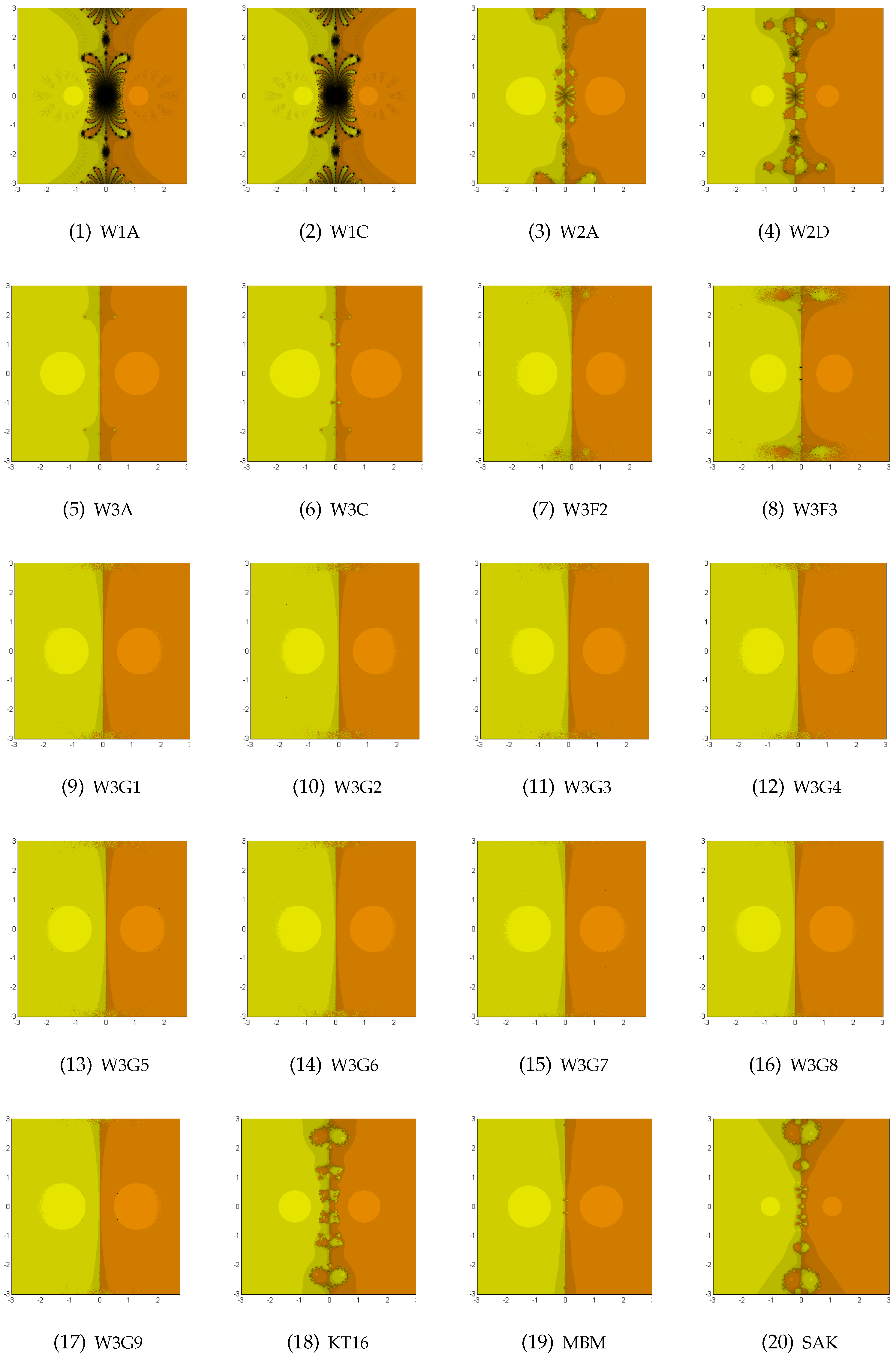
We have taken as a quadratic polynomial with all real roots:
The roots are obviously . Note that the extraneous fixed points are computed based on this example. Clearly the best methods have basins separated by the imaginary axis. Basins of attraction for W1A–W3G9, KT16, MBM with and SAK are given in Figure 1. Methods W3A, W3G1–W3G8 show basins separated by the imaginary axis. Consulting Table 5, Table 6 and Table 7, we find that the methods W3G7–W3G9 use the least number of iterations per point on average (ANIP), followed closely by W3C, W3G1, W3G3–W3G6. The fastest method is W3A. The methods KT16, MBM, and SAK have the least number of black points. Methods W1A and W1C have the highest number of black points. Notice that these methods use polynomial weight functions.
Example2.
We have taken as a cubic polynomial:
Basins of attraction are given in Figure 2. Notice that the basins for W1A and W1C have many black points and therefore will not be considered in the rest of the examples. Besides that, in view of a close inspection that the basins for W3G3–W3G6 have similarities to the other remaining members of the listed W3G-family, we will omit them in the rest of the examples. Consulting Table 5, Table 6 and Table 7, we find that the method with the fewest ANIP is MBM with 2.22 iteration. All the others require between 2.71 and 12.12. In terms of CPU timein seconds, the fastest is W3A (472.715 s) and the slowest is W1C (2399.093 s). The methods W1C and W1A have the most black points (59,904 and 58,910, respectively) and SAK has the least number (6 points). We will not consider W1A and W1C any further.
Example3.
We have taken as another cubic polynomial:
All roots were easily found to be real. The basins for this example are plotted in Figure 3. The basins for W2A, W2D, KT16, and SAK are too chaotic. Based on Table 5 we see that W3C has the lowest ANIP followed closely by MBM. The fastest method is again W3A (406.102 s) and the slowest is W3G8 (2041.663 seconds). The methods KT16, MBM, and SAK have no black points, and the rest have between 58 and 204 black points.
Example4.
We have taken as a quartic polynomial:
The basins are given in Figure 4. We now see that W2A is the worst, followed by W2D. The best are those with smaller lobes along the diagonals. In terms of ANIP, W3C is the best (2.58), followed by MBM (2.64), and the worst is W2A (25.22). The fastest is again W3A (497.284 s), followed by W3C (542.509 s), and the slowest is W2A (5117.503 s). Most of the methods have between 1201 and 1889 black points with the worst being W2A with 218,849 points and W2D with 10,785 black points. We remove W2A from further consideration.
Example5.
We have taken as a quintic polynomial:
The basins for the best methods left are plotted in Figure 5. The worst are W3A, W2D, and SAK. In terms of ANIP, the best is W3C (2.64), followed closely by MBM (2.76), and the worst are W3A (7.91) and SAK (5.40). The fastest is W3C using 615.892 s, followed by KT16 using 888.784 s, and the slowest was W3G1 (2409.685 s). SAK has 18 black points, but the basins are chaotic. The highest number of black points is for W3A (49,176), preceded by W2D with 13,828 black points. We remove W2D from further consideration.
Example6.
We have taken as a sextic polynomial with complex coefficients:
The basins for the best methods left are plotted in Figure 6. It is clear that the SAK is very chaotic. Based on Table 5, we find that MBM has the lowest ANIP (2.41) followed by KT16 (3.92). The fastest method is W3C (1869.921 s), followed by MBM (2045.282 s), and W3A (2199.567 s). The slowest is SAK taking 2947.202 s. There are two methods with five black points or fewer, namely, SAK and MBM. The highest number is for W3G2 with 36,697 black points. In fact, all our new methods have over 29,000 black points.
Example7.
We have taken as a nonpolynomial equation:
The basins for this example are plotted in Figure 7. The roots are at and it is expected that the boundary will be close to the imaginary axis as in Example 1. All methods show a larger basin for the root at . The methods with the largest basin for are W3A, W3C, and MBM. In terms of ANIP, MBM was best (2.02), followed closely by W3A (2.17) and W3C (2.19). The worst is SAK with 3.83. The fastest method is W3A (461.358 s) and the slowest is MBM (923.011 s). MBM has the least number of black points (644) and SAK has the highest (13720) such number.
We now average all these results across the seven examples to try and pick the best method. MBM had the lowest ANIP (2.34), followed by W3C with 2.88. The fastest method was W3C (695.931 s), followed by W3A (847.596 s). MBM has the lowest number of black points on average (705), followed by KT16 (1101 black points).
Based on these seven examples we see that MBM and W3C have three examples with the lowest ANIP, W3G7, W3G8, and W3G9 each with one example. W3A is the fastest in five examples and W3C in two examples. Thus, we recommend W3C and W3G7, since W3C is in the top four and W3G7 in the top five in all three categories. MBM was at the top in only two categories, KT16 is in top three in two categories, and W3F3 and W3G9 were in the top six in two categories.
5. Conclusions
Both numerical and dynamical aspects of Iterative Maps (5) support the main theorem well through a number of test equations and examples. The W3F and W3G methods were observed to occupy relatively slower CPU time due to the intensive use of rational coefficients for weight function . If less number of the rational coefficients were employed, it would take less CPU time to build the relevant basins of attraction.
The proposed Family of Methods (5) favorably cover most of optimal sixteenth-order simple-root finders with certain weight functions developed (or to be developed), since they employ fairly generic weight functions. The dynamics behind the purely imaginary extraneous fixed points will choose best members of the family with improved convergence behavior. However, due to the order of convergence is rather high, the required algebra encounters difficulty resolving its increased complexity. The current work is limited to univariate nonlinear equations; its extension to multivariate ones becomes another task. In future work, as a follow-up study, we will not only extend Case 3 with other combinations of simple coefficients , but also investigate different types of weight functions possessing less number of rational coefficients to obtain purely imaginary extraneous fixed points, and strengthen the desired computational as well as dynamical behavior.
Author Contributions
Investigation, Y.H.G.; analysis and writing, Y.I.K.; analysis and supervision, B.N.
Funding
The first author (Y.H. Geum) was supported by the Basic Science Research Program through the National Research Foundation of Korea funded by the Ministry of Education under research grant Project Number: NRF-2018R1D1A1B07047715.
Conflicts of Interest
The authors have no conflict of interest to declare.
References
Bi, W.; Wu, Q.; Ren, H. A new family of eighth-order iterative methods for solving nonlinear equations. Appl. Math. Comput.2009, 214, 236–245. [Google Scholar] [CrossRef]
Chun, C.; Neta, B. Comparative study of eighth order methods for finding simple roots of nonlinear equations. Numer. Algorithms2017, 74, 1169–1201. [Google Scholar] [CrossRef]
Geum, Y.H.; Kim, Y.I. A uniparametric family of three-step eighth-order multipoint iterative methods for simple roots. Appl. Math. Lett.2011, 24, 929–935. [Google Scholar] [CrossRef]
Lee, S.D.; Kim, Y.I.; Neta, B. An optimal family of eighth-order simple-root finders with weight functions dependent on function-to-function ratios and their dynamics underlying extraneous fixed points. J. Comput. Appl. Math.2017, 317, 31–54. [Google Scholar] [CrossRef] [Green Version]
Liu, L.; Wang, X. Eighth-order methods with high efficiency index for solving nonlinear equations. Appl. Math. Comput.22010, 15, 3449–3454. [Google Scholar] [CrossRef]
Džunić, J.; Petković, M.S.; Petković, L.D. A family of optimal three-point methods for solving nonlinear equations using two parametric functions. Appl. Math. Comput.2011, 217, 7612–7619. [Google Scholar] [CrossRef]
Petković, M.S.; Neta, B.; Petković, L.D.; Džunić, J. Multipoint Methods for Solving Nonlinear Equations; Elsevier: New York, NY, USA, 2012. [Google Scholar]
Petković, M.S.; Neta, B.; Petković, L.D.; Džunić, J. Multipoint methods for solving nonlinear equations: A survey. Appl. Math. Comput.2014, 226, 635–660. [Google Scholar] [CrossRef] [Green Version]
Sharma, J.R.; Arora, H. A new family of optimal eighth order methods with dynamics for nonlinear equations. Appl. Math. Comput.2016, 273, 924–933. [Google Scholar] [CrossRef]
Traub, J.F. Iterative Methods for the Solution of Equations; Chelsea Publishing Company: Chelsea, VT, USA, 1982. [Google Scholar]
Kung, H.T.; Traub, J.F. Optimal order of one-point and multipoint iteration. J. Assoc. Comput. Mach.1974, 21, 643–651. [Google Scholar] [CrossRef]
Maroju, P.; Behl, R.; Motsa, S.S. Some novel and optimal families of King’s method with eighth and sixteenth-order of convergence. J. Comput. Appl. Math.2017, 318, 136–148. [Google Scholar] [CrossRef]
Sharma, J.R.; Argyros, I.K.; Kumar, D. On a general class of optimal order multipoint methods for solving nonlinear equations. J. Math. Anal. Appl.2017, 449, 994–1014. [Google Scholar] [CrossRef]
Ahlfors, L.V. Complex Analysis; McGraw-Hill Book, Inc.: New York, NY, USA, 1979. [Google Scholar]
Hörmander, L. An Introduction to Complex Analysis in Several Variables; North-Holland Publishing Company: Amsterdam, The Netherlands, 1973. [Google Scholar]
Shabat, B.V. Introduction to Complex Analysis PART II, Functions of Several Variables; American Mathematical Society: Providence, RI, USA, 1992. [Google Scholar]
Neta, B. On a family of Multipoint Methods for Non-linear Equations. Int. J. Comput. Math.1981, 9, 353–361. [Google Scholar] [CrossRef]
Devaney, R.L. An Introduction to Chaotic Dynamical Systems; Addison-Wesley Publishing Company, Inc.: Boston, MA, USA, 1987. [Google Scholar]
Vrscay, E.R.; Gilbert, W.J. Extraneous Fixed Points, Basin Boundaries and Chaotic Dynamics for shröder and König rational iteration Functions. Numer. Math.1988, 52, 1–16. [Google Scholar] [CrossRef]
Wolfram, S. The Mathematica Book, 5th ed.; Wolfram Media: Champaign, IL, USA, 2003. [Google Scholar]
Geum, Y.H.; Kim, Y.I.; Neta, B. Constructing a family of optimal eighth-order modified Newton-type multiple-zero finders along with the dynamics behind their purely imaginary extraneous fixed points. J. Comput. Appl. Math.2018, 333, 131–156. [Google Scholar] [CrossRef]
Rhee, M.S.; Kim, Y.I.; Neta, B. An optimal eighth-order class of three-step weighted Newton’s methods and their dynamics behind the purely imaginary extraneous fixed points. Int. J. Comput. Math.2017, 95, 2174–2211. [Google Scholar] [CrossRef]
Stewart, B.D. Attractor Basins of Various Root-Finding Methods. Master’s Thesis, Naval Postgraduate School, Department of Applied Mathematics, Monterey, CA, USA, June 2001. [Google Scholar]
Amat, S.; Busquier, S.; Plaza, S. Review of some iterative root-finding methods from a dynamical point of view. Scientia2004, 10, 3–35. [Google Scholar]
Amat, S.; Busquier, S.; Plaza, S. Dynamics of the King and Jarratt iterations. Aequ. Math.2005, 69, 212–223. [Google Scholar] [CrossRef]
Andreu, C.; Cambil, N.; Cordero, A.; Torregrosa, J.R. A class of optimal eighth-order derivative-free methods for solving the Danchick-Gauss problem. Appl. Math. Comput.2014, 232, 237–246. [Google Scholar] [CrossRef]
Argyros, I.K.; Magreñán, A.Á. On the convergence of an optimal fourth-order family of methods and its dynamics. Appl. Math. Comput.2015, 252, 336–346. [Google Scholar] [CrossRef]
Chun, C.; Lee, M.Y.; Neta, B.; Dz̆unić, J. On optimal fourth-order iterative methods free from second derivative and their dynamics. Appl. Math. Comput.2012, 218, 6427–6438. [Google Scholar] [CrossRef] [Green Version]
Chun, C.; Neta, B. Comparison of several families of optimal eighth order methods. Appl. Math. Comput.2016, 274, 762–773. [Google Scholar] [CrossRef] [Green Version]
Geum, Y.H.; Kim, Y.I.; Magreñán, Á.A. A biparametric extension of King’s fourth-order methods and their dynamics. Appl. Math. Comput.2016, 282, 254–275. [Google Scholar] [CrossRef]
Geum, Y.H.; Kim, Y.I.; Neta, B. A class of two-point sixth-order multiple-zero finders of modified double-Newton type and their dynamics. Appl. Math. Comput.2015, 270, 387–400. [Google Scholar] [CrossRef] [Green Version]
Geum, Y.H.; Kim, Y.I.; Neta, B. A sixth-order family of three-point modified Newton-like multiple-root finders and the dynamics behind their extraneous fixed points. Appl. Math. Comput.2016, 283, 120–140. [Google Scholar] [CrossRef] [Green Version]
Magreñan, Á.A. Different anomalies in a Jarratt family of iterative root-finding methods. Appl. Math. Comput.2014, 233, 29–38. [Google Scholar]
Magreñan, Á.A. A new tool to study real dynamics: The convergence plane. Appl. Math. Comput.2014, 248, 215–224. [Google Scholar] [CrossRef] [Green Version]
Neta, B.; Scott, M.; Chun, C. Basins of attraction for several methods to find simple roots of nonlinear equations. Appl. Math. Comput.2012, 218, 10548–10556. [Google Scholar] [CrossRef] [Green Version]
Neta, B.; Scott, M.; Chun, C. Basin attractors for various methods for multiple roots. Appl. Math. Comput.2012, 218, 5043–5066. [Google Scholar] [CrossRef] [Green Version]
Neta, B.; Chun, C.; Scott, M. Basins of attraction for optimal eighth order methods to find simple roots of nonlinear equations. Appl. Math. Comput.2014, 227, 567–592. [Google Scholar] [CrossRef]
Scott, M.; Neta, B.; Chun, C. Basin attractors for various methods. Appl. Math. Comput.2011, 218, 2584–2599. [Google Scholar] [CrossRef] [Green Version]
Chun, C.; Neta, B.; Kozdon, J.; Scott, M. Choosing weight functions in iterative methods for simple roots. Appl. Math. Comput.2014, 227, 788–800. [Google Scholar] [CrossRef] [Green Version]
Chun, C.; Neta, B. Basins of attraction for Zhou-Chen-Song fourth order family of methods for multiple roots. Math. Comput. Simul.2015, 109, 74–91. [Google Scholar] [CrossRef]
Neta, B.; Chun, C. Basins of attraction for several optimal fourth order methods for multiple roots. Math. Comput. Simul.2014, 103, 39–59. [Google Scholar] [CrossRef] [Green Version]
Beardon, A.F. Iteration of Rational Functions; Springer: New York, NY, USA, 1991. [Google Scholar]
Figure 1.
The top row for W1A (left), W1C (center left), W2A (center right) and W2D (right). The second row for W3A (left), W3C (center left), W3F2 (center right) and W3F3 (right). The third row for W3G1 (left), W3G2 (center left), W3G3 (center right), and W3G4 (right). The fourth row for W3G5 (left), W3G6 (center left), W3G7 (center right), and W3G8 (right). The bottom row for W3G9 (left), KT16 (center left), MBM (center right) and SAK (right), for the roots of the polynomial equation (z2 − 1).
Figure 2.
The top row for W1A (left), W1C (center left), W2A (center right) and W2D (right). The second row for W3A (left), W3C (center left), W3F2 (center right), and W3F3 (right). The third row for W3G1 (left), W3G2 (center left), W3G7 (center right), and W3G8 (right). The bottom row for W3G9 (left), KT16 (center left), MBM (center right) and SAK (right), for the roots of the polynomial equation ().
Figure 3.
The top row for W2A (left), W2D (center left), W3A (center right) and W3C (right). The second row for W3F2 (left), W3F3 (center left), W3G1 (center right), and W3G2 (right). The third row for W3G7 (left), W3G8 (center left), W3G9 (center right), and KT16 (right). The bottom row for MBM (left), SAK (center left), for the roots of the polynomial equation ().
Figure 4.
The top row for W2A (left), W2D (center left), W3A (center right), and W3C (right). The second row for W3F2 (left), W3F3 (center left), W3G1 (center right), and W3G2 (right). The third row for W3G7 (left), W3G8 (center left), W3G9 (center right), and KT16 (right). The bottom row for MBM (left), SAK (center left), for the roots of the polynomial equation ().
Figure 5.
The top row for W2D (left), W3A (center left), W3C (center right) and W3F2 (right). The second row for W3F3 (left), W3G1 (center left), W3G2 (center right) and W3G7 (right). The third row for W3G8 (left), W3G9 (center left), KT16 (center right) and MBM (right). The bottom row for SAK (center), for the roots of the polynomial equation ().
Figure 6.
The top row for W3A (left), W3C (center left), W3F2 (center right), and W3F3 (right). The second row for W3G1 (left), W3G2 (center left), W3G7 (center right), and W3G8 (right). The bottom row for W3G9 (left), KT16 (center left), and MBM (center right) and SAK (right), for the roots of the polynomial equation .
Figure 7.
The top row for W3A (left), W3C (center left), W3F2 (center right), and W3F3 (right). The second row for W3G1 (left), W3G2 (center left), W3G7 (center right), and W3G8 (right). The bottom row for W3G9 (left), KT16 (center left), and MBM (center right) and SAK (right), for the roots of non-polynomial equation ().
Table 1.
Indifferent extraneous fixed points for selected cases.
Table 1.
Indifferent extraneous fixed points for selected cases.
Case
No. of
1A
84
1B
148
1C
116
1D
148
2A
58
2B
66
2C
62
2D
54
2E
62
2F
62
2G
58
3A
24
3B
26
3C
30
3D
30
3E
14
3F1
14
3F2
14
3F3
14
3G
14
KT16
118
MBM
22
SAK
14
The highlighted methods are investigated for their dynamics in Section 5.
Table 2.
Convergence of methods W3G1, W2D, W1C for test functions shown in (72).
Table 2.
Convergence of methods W3G1, W2D, W1C for test functions shown in (72).
F
n
0
1.8
0.270467
0.0715473
W3G1
1
1.72845267553040
16.3348
2
1.72845267553040
16.00000
0
1.3
0.806294
0.270796
W2D
1
1.57079632679455
0.0004131418075
12.6338
2
1.57079632679490
16.00000
0
0.198116
0.0572814
W1C
1
103591.4791
3210.28764
14.7852
2
3210.287640
16.00000
MT = method, , , .
Table 3.
Additional test functions with zeros and initial values .
Table 3.
Additional test functions with zeros and initial values .
i
1
2
3
4
0
5
6
7
Here, .
Table 4.
Comparison of for selected methods applied to various test functions.
Table 4.
Comparison of for selected methods applied to various test functions.
Method
W1A
1.27e-17
1.16e-14
1.26e-12
2.12e-19
3.06e-14
2.49e-13
3.89e-20
2.32e-278
1.74e-222
1.40e-187
2.04e-299
6.71e-221
3.55e-203
2.38e-322
W1B
2.64e-17
1.75e-14
1.42e-12
5.21e-19
3.18e-14
3.62e-13
1.01e-19
5.35e-273
1.68e-219
1.34e-186
4.14e-293
2.17e-220
2.41e-200
5.02e-316
W1C
1.13e-17
1.47e-14
3.25e-13
6.36e-18
5.31e-14
2.425e-13
6.72e-21
3.73e-279
1.08e-220
5.78e-197
1.79e-276
4.06e-217
2.10e-203
2.03e-336
W1D
1.05e-17
1.58e-14
6.86e-14
4.28e-19
1.42e-14
1.72e-13
2.21e-19
1.24e-279
4.94e-220
9.10e-208
5.24e-296
3.17e-226
9.51e-206
1.51e-309
W2A
2.24e-16
3.82e-17
1.48e-11
1.01e-17
1.78e-10
5.71e-13
3.33e-17
4.22e-261
2.86e-265
4.11e-173
4.96e-273
1.27e-161
2.58e-199
1.42e-271
W2B
2.70e-16
1.739e-17
1.04e-11
4.740e-18
1.26e-10
7.65e-13
2.74e-17
8.30e-260
3.33e-271
9.27e-176
2.15e-278
4.22e-164
2.51e-197
4.84e-273
W2C
1.88e-16
8.79e-17
1.79e-11
1.82e-17
1.94e-10
4.57e-13
3.57e-17
2.66e-262
6.78e-259
1.65e-171
1.09e-268
4.42e-161
8.62e-201
4.62e-271
W2D
2.66e-16
1.53e-17
8.09e-12
5.94e-18
9.75e-11
7.73e-13
2.36e-17
6.67e-260
7.71e-272
1.61e-177
7.60e-277
3.22e-166
3.33e-197
4.05e-274
W2E
2.58e-16
1.26e-17
1.33e-11
2.81e-17
1.49e-10
7.09e-13
2.72e-17
4.10e-260
1.28e-273
4.35e-174
1.07e-265
3.37e-163
8.28e-198
4.97e-273
W2F
2.26e-16
3.98e-17
1.37e-11
5.19e-18
1.68e-10
5.83e-13
3.30e-17
4.96e-261
4.51e-265
1.26e-173
9.26e-278
5.57e-162
3.46e-199
1.20e-271
W2G
2.33e-16
3.32e-17
1.37e-11
8.62e-18
1.64e-10
6.08e-13
3.19e-17
7.83e-261
2.51e-266
1.04e-173
3.71e-274
3.52e-162
6.92e-199
6.87e-272
W3A
2.17e-16
2.12e-18
1.13e-13
3.62e-18
4.97e-12
6.73e-13
2.86e-18
2.68e-261
2.61e-287
1.73e-207
2.69e-280
3.36e-186
6.01e-198
5.10e-290
W3B
2.25e-16
2.28e-18
1.11e-13
2.50e-18
6.75e-12
7.18e-13
3.60e-18
5.05e-261
1.10e-286
1.25e-207
6.12e-283
4.66e-184
1.71e-197
2.77e-288
W3C
2.32e-16
2.19e-18
1.34e-13
2.45e-18
9.99e-12
7.52e-13
4.72e-18
8.27e-261
4.83e-287
2.53e-206
4.40e-283
2.59e-181
3.59e-197
3.15e-286
W3D
2.39e-16
2.11e-18
1.54e-13
2.41e-18
1.26e-11
7.82e-13
5.91e-18
1.30e-260
2.06e-287
2.32e-205
3.25e-283
1.12e-179
6.77e-197
1.54e-284
W3E
7.41e-17
1.13e-18
4.49e-14
1.90e-18
1.77e-12
3.37e-13
4.80e-18
4.02e-270
1.05e-291
2.58e-214
6.03e-285
6.04e-194
2.06e-203
3.05e-286
W3F1
7.07e-14
1.39e-15
1.28e-11
3.41e-15
2.01e-10
7.64e-11
2.15e-15
3.46e-217
5.18e-238
2.57e-170
2.01e-228
1.23e-156
3.56e-161
5.70e-240
W3F2
4.43e-14
9.32e-16
9.06e-12
2.25e-15
1.02e-10
5.04e-11
1.18-15
1.47e-220
6.99e-241
8.64e-173
2.16e-231
1.92e-161
3.48e-164
2.74e-244
W3F3
8.02e-15
3.45e-16
3.67e-12
6.84e-16
6.30e-11
1.12e-11
7.51e-17
1.94e-233
5.93e-248
2.36e-179
5.94e-240
4.88e-166
2.03e-176
3.93e-264
W3G1
8.11e-13
2.78e-14
6.06e-11
5.85e-14
2.54e-10
4.74e-10
7.06e-15
3.52e-200
4.29e-217
2.41e-159
1.64e-208
4.75e-155
1.82e-148
9.27e-233
W3G2
3.18e-13
4.15e-15
4.17e-11
1.54e-14
1.42e-10
8.29e-10
4.21e-15
8.83e-206
1.95e-229
4.46e-161
6.62e-217
3.96e-158
1.15e-143
4.83e-235
W3G3
2.88e-12
1.32e-14
5.92e-11
8.83e-13
2.35e-10
6.92e-10
2.34e-14
2.73e-191
3.53e-222
1.98e-159
1.42e-189
1.72e-155
9.65e-146
6.62e-225
W3G4
2.04e-12
1.44e-14
5.95e-11
2.68e-13
2.38e-10
6.44e-10
1.73e-14
1.06e-193
1.42e-221
2.12e-159
7.32e-198
2.10e-155
2.95e-146
7.47e-227
W3G5
9.79e-13
2.20e-14
6.04e-11
7.52e-14
2.50e-10
5.12e-10
8.57e-15
7.45e-199
1.09e-218
2.42e-159
9.37e-207
3.89e-155
6.68e-148
1.79e-231
W3G6
9.07e-13
2.39e-14
6.05e-11
6.78e-14
2.51e-10
4.97e-10
7.92e-15
2.15e-199
4.05e-218
2.43e-159
1.75e-207
4.21e-155
4.01e-148
5.44e-232
W3G7
1.27e-14
1.00e-17
2.97e-12
1.05e-16
3.57e-10
1.38e-11
9.64e-16
4.98e-230
3.62e-274
5.80e-182
2.63e-254
2.21e-153
7.26e-174
5.88e-246
W3G8
2.07e-14
1.82e-16
1.74e-12
5.40e-16
3.62e-10
2.49e-11
1.04e-15
1.77e-226
2.62e-253
3.10e-185
2.59e-242
3.46e-153
1.19e-169
2.27e-245
W3G9
2.34e-14
2.40e-16
1.80e-12
6.90e-16
3.64e-10
2.88e-11
1.07e-15
1.45e-225
2.83e-251
6.66e-185
1.64e-240
4.02e-153
1.32e-168
3.55e-245
KT16
5.62e-17
4.41e-17
1.87e-12
1.85e-19
1.47e-13
2.44e-13
6.41e-19
7.30e-273
4.73e-264
3.87e-187
1.11e-300
1.31e-211
1.42e-206
4.32e-301
MBM
5.81e-17
2.81e-17
2.30e-12
8.74e-20
5.26e-12
1.12e-13
9.07e-18
1.64e-270
5.23e-268
7.95e-186
6.25e-306
7.47e-186
3.34e-210
1.47e-281
SAK
7.41e-17
1.13e-18
4.49e-14
1.90e-18
1.77e-12
3.37e-13
4.80e-18
4.02e-270
1.05e-291
2.58e-214
6.03e-285
6.04e-194
2.06e-203
3.05e-286
1.27e-17 .
Table 5.
Average number of iterations per point for each example (1–7).
Table 5.
Average number of iterations per point for each example (1–7).
Example
Map
1
2
3
4
5
6
7
Average
W1A
4.00
11.90
-
-
-
-
-
-
W1C
4.08
12.12
-
-
-
-
-
-
W2A
2.24
3.27
3.53
25.22
-
-
-
-
W2D
2.46
3.56
2.82
5.11
4.92
-
-
-
W3A
2.04
2.86
2.30
2.70
7.91
6.59
2.17
3.80
W3C
2.02
2.82
2.24
2.58
2.64
5.65
2.19
2.88
W3F2
2.07
2.89
2.47
2.80
2.91
6.47
2.38
3.14
W3F3
2.21
2.72
2.45
2.77
2.86
6.18
2.34
3.08
W3G1
2.02
2.95
2.51
2.89
3.02
6.69
2.54
3.23
W3G2
2.03
2.98
2.50
2.88
2.99
6.67
2.48
3.22
W3G3
2.02
2.94
-
-
-
-
-
-
W3G4
2.02
2.94
-
-
-
-
-
-
W3G5
2.02
2.94
-
-
-
-
-
-
W3G6
2.02
2.93
-
-
-
-
-
-
W3G7
2.01
2.82
2.37
2.78
2.82
6.06
2.27
3.02
W3G8
2.01
2.84
2.40
2.83
2.88
6.18
2.37
3.07
W3G9
2.01
2.82
2.41
2.83
2.89
6.26
2.38
3.09
KT16
2.31
3.02
2.76
3.83
3.99
3.92
2.45
3.18
MBM
2.04
2.22
2.28
2.64
2.76
2.41
2.02
2.34
SAK
2.35
2.76
3.02
3.78
5.40
4.50
3.83
3.66
Table 6.
CPU time (in seconds) required for each example(1–7) using a Dell Multiplex-990.
Table 6.
CPU time (in seconds) required for each example(1–7) using a Dell Multiplex-990.
Example
Map
1
2
3
4
5
6
7
Average
W1A
631.680
2331.092
-
-
-
-
-
-
W1C
635.548
2399.093
-
-
-
-
-
-
W2A
380.768
604.769
695.952
5117.503
-
-
-
-
W2D
446.646
664.393
582.336
1123.160
1143.846
-
-
-
W3A
316.370
472.715
406.102
497.284
1579.775
2199.567
461.358
847.596
W3C
354.466
529.495
451.421
542.509
615.892
1869.921
507.815
695.931
W3F2
561.791
850.642
771.487
843.607
948.190
2371.028
786.229
1018.996
W3F3
628.418
795.964
798.741
849.410
933.650
2378.079
785.855
1024.302
W3G1
541.432
820.160
726.855
836.680
978.782
2557.308
806.525
1038.249
W3G2
545.754
828.677
739.960
863.824
934.306
2553.424
799.552
1037.928
W3G3
575.986
575.986
-
-
-
-
-
-
W3G4
555.738
851.375
-
-
-
-
-
-
W3G5
577.750
867.132
-
-
-
-
-
-
W3G6
573.116
836.446
-
-
-
-
-
-
W3G7
562.321
809.676
724.812
828.927
896.834
2385.099
768.789
996.637
W3G8
557.828
803.140
720.288
837.039
909.143
2552.878
772.424
1021.820
W3G9
551.416
784.529
715.530
824.590
936.240
2462.929
770.333
1006.510
KT16
386.414
679.572
529.482
783.359
888.784
2427.189
564.770
894.224
MBM
831.189
1039.919
993.804
1157.589
1205.014
2045.282
923.011
1170.830
SAK
467.785
712.831
687.824
833.653
1376.600
2947.202
849.831
1125.104
Table 7.
Number of points requiring 40 iterations for each example (1–7).
Table 7.
Number of points requiring 40 iterations for each example (1–7).
Geum, Y.H.; Kim, Y.I.; Neta, B.
Developing an Optimal Class of Generic Sixteenth-Order Simple-Root Finders and Investigating Their Dynamics. Mathematics2019, 7, 8.
https://doi.org/10.3390/math7010008
AMA Style
Geum YH, Kim YI, Neta B.
Developing an Optimal Class of Generic Sixteenth-Order Simple-Root Finders and Investigating Their Dynamics. Mathematics. 2019; 7(1):8.
https://doi.org/10.3390/math7010008
Chicago/Turabian Style
Geum, Young Hee, Young Ik Kim, and Beny Neta.
2019. "Developing an Optimal Class of Generic Sixteenth-Order Simple-Root Finders and Investigating Their Dynamics" Mathematics 7, no. 1: 8.
https://doi.org/10.3390/math7010008
APA Style
Geum, Y. H., Kim, Y. I., & Neta, B.
(2019). Developing an Optimal Class of Generic Sixteenth-Order Simple-Root Finders and Investigating Their Dynamics. Mathematics, 7(1), 8.
https://doi.org/10.3390/math7010008
Note that from the first issue of 2016, this journal uses article numbers instead of page numbers. See further details here.
Article Metrics
No
No
Article Access Statistics
For more information on the journal statistics, click here.
Multiple requests from the same IP address are counted as one view.
Geum, Y.H.; Kim, Y.I.; Neta, B.
Developing an Optimal Class of Generic Sixteenth-Order Simple-Root Finders and Investigating Their Dynamics. Mathematics2019, 7, 8.
https://doi.org/10.3390/math7010008
AMA Style
Geum YH, Kim YI, Neta B.
Developing an Optimal Class of Generic Sixteenth-Order Simple-Root Finders and Investigating Their Dynamics. Mathematics. 2019; 7(1):8.
https://doi.org/10.3390/math7010008
Chicago/Turabian Style
Geum, Young Hee, Young Ik Kim, and Beny Neta.
2019. "Developing an Optimal Class of Generic Sixteenth-Order Simple-Root Finders and Investigating Their Dynamics" Mathematics 7, no. 1: 8.
https://doi.org/10.3390/math7010008
APA Style
Geum, Y. H., Kim, Y. I., & Neta, B.
(2019). Developing an Optimal Class of Generic Sixteenth-Order Simple-Root Finders and Investigating Their Dynamics. Mathematics, 7(1), 8.
https://doi.org/10.3390/math7010008
Note that from the first issue of 2016, this journal uses article numbers instead of page numbers. See further details here.


