Article

A Statistical Investigation into Assembly Tolerances of Gradient Field Magnetic Angle Sensors with Hall Plates

1
Infineon Technologies Austria AG, 9500 Villach, Austria
2
Institut für Intelligente Systemtechnologien, Alpen Adria Universitaet Klagenfurt, 9020 Klagenfurt, Austria
*
Author to whom correspondence should be addressed.
These authors contributed equally to this work.
Current address: Siemensstrasse 2, 9500 Villach, Austria.
Mathematics 2019, 7(10), 968; https://doi.org/10.3390/math7100968
Submission received: 11 September 2019 / Revised: 2 October 2019 / Accepted: 8 October 2019 / Published: 14 October 2019
(This article belongs to the Special Issue Recent Advances in Modeling for Reliability Analysis)

Abstract

:
Magnetic field-based sensors are used for reliable applications in automotive and aerospace industry because of their robustness. The electrification of powertrains and propulsion requires gradiometric sensing principles, because they suppress ubiquitous electromagnetic disturbances very efficiently. A prominent solution for the mass market uses a small permanent magnet attached to the end of a rotatable shaft and a small sensor chip with four Hall plates placed on the rotation axis and ahead of the magnet. Small misplacements of chip and magnet lead to errors in the detected angle of the shaft. The lateral position errors and tilts of the magnet and the chip give eight degrees of freedom (DoF). This large number of DoF and the nonlinearity of the system obscure the view on how to optimize such angle sensor systems. Therefore, this work presents a statistical description of angle errors caused by assembly tolerances. Probability distributions of angle errors are given and marked differences to Gaussian distributions are shown. The influence of spacing between sensor and magnet and the dominant influence of the shape of the magnet are clarified. The results obtained by numerical computations are in excellent agreement to recently published analytical theories. This work gives evident conclusions for statistical optimizations of such angle sensor systems.

1. Introduction

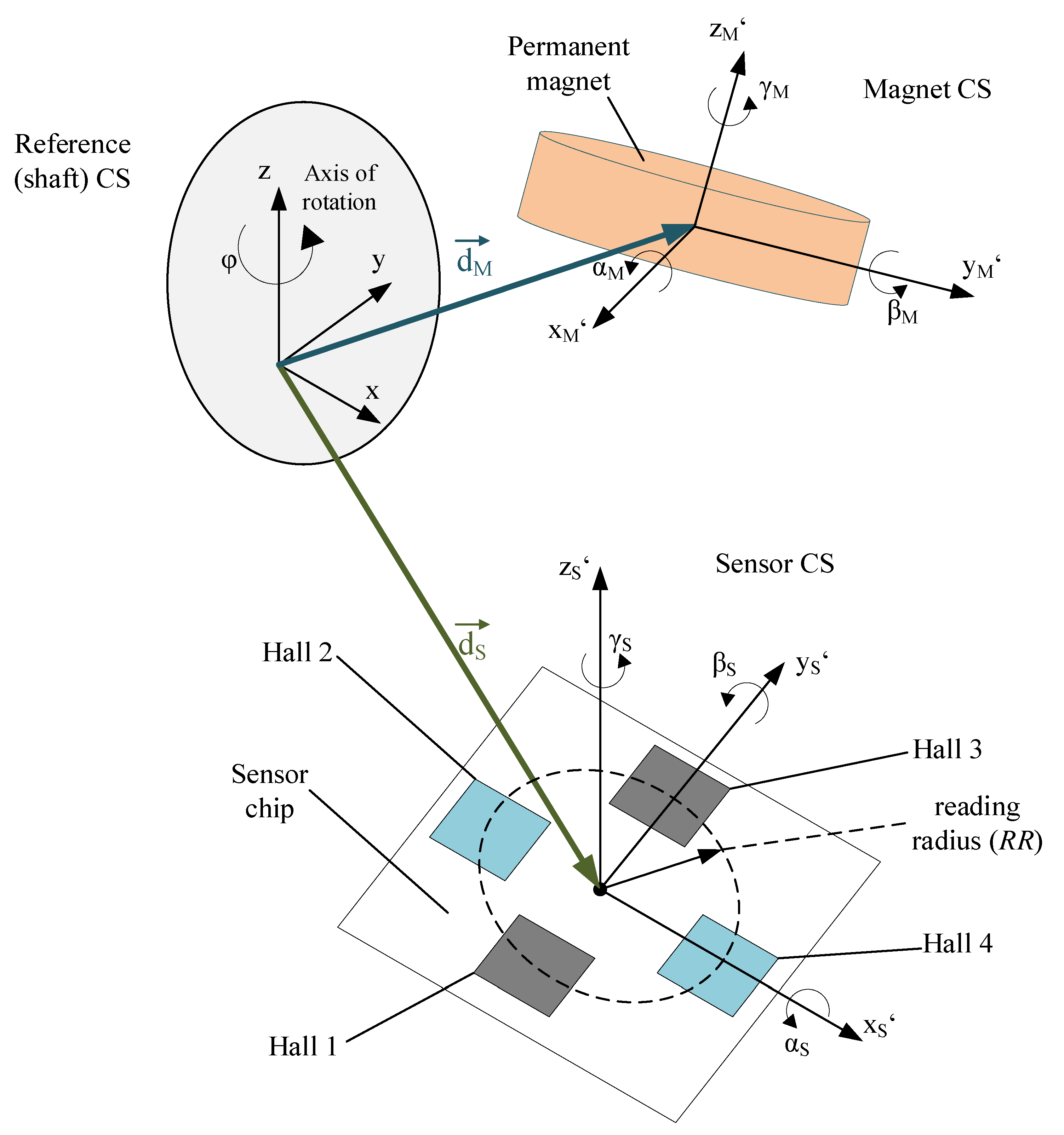
Magnetic sensing principles are well established in the automotive industry because of their robust and reliable operation without abrasion, even in dirty environments [1]. The automotive sector is presently moving from combustion engines to electric driven propulsion with high-power cables causing electromagnetic interference (EMI) to other electromagnetic sensitive devices inside a car. The trend for safe and autonomous systems, on the other hand, increases the number of sensors and actuators inside a vehicle, which therefore have to be smaller and more robust and reliable. Such magnetic angle sensors for 360 detection are traditionally made with magnetoresistive sensors (e.g., GMRand TMR) [2,3] or with vertical Hall-effect devices. Their angle accuracy is limited roughly to ∼0.3 …∼1 by the assembly tolerances of the sensor and magnet with respect to the rotation axis [4,5,6]. Their main limitation nowadays is that relatively small magnetic disturbance fields of 5 mT give large errors of 5 . In-shaft magnetic angle sensing solves these problems and improves the angle accuracy to ∼0.2 [7]. There the angle sensor devices are placed in the center of a cheap ferrite injection molded Halbach ring magnet inside the bore of a ferrous shaft, which perfectly shields external disturbances. Due to the high symmetry of the field in the Halbach magnet, assembly tolerances lead only to very small angle errors. Another strategy to cope with disturbance fields is to use gradiometric magnetic sensors. They are cheaper, because they need no magnetic shielding, and they need only smaller, simpler magnets. The basic principle of a widely used angle sensor system with Hall plates is described in [8], but the idea dates back to [9]. A similar system was developed in [10]. Other angle sensor systems add small magnetic fluxguides or concentrators on the sensor chip [11]. However, these are not gradiometers, and therefore they do not cancel out disturbances of external magnetic fields. Yet, this basic principle can be used to construct more complex gradiometers with robustness against disturbance fields [12]. Unfortunately, it can be shown that gradiometric sensors are less robust against assembly tolerances than systems that respond to homogeneous magnetic fields [13]. This is not a consequence of the sensing elements (e.g., TMRs or Hall plates). It is caused by the gradiometric sensing principle itself: gradients are less homogeneous than absolute field values, and therefore they are more prone to placement tolerances. This is explained in Chapter 7 of [14] with a thorough comparison of all common magnetic sensor technologies. Apart from permanent magnetic angle sensors also inductive angle sensors are known [15]. They are very accurate and robust against electromagnetic disturbances, and they are well suited for through-shaft arrangements, where the end of a shaft is not available. However, they are more complex and expensive for full 360 detection and they need more space (diameters > 30 mm). The purpose of this paper is to look at the statistical distribution of angle errors of gradiometric angle sensors of type [8] and to indicate how the angle accuracy can be optimized. In our case, the magnetic field component perpendicular to a chip is detected by four Hall plates, which are located at 0 , 90 , 180 , and 270 on a circle [8]. The radius of the circle is called the reading radius, R R . A schematic overview of this sensing principle is shown in Figure 1.
Two opposite Hall plates make up one gradiometer, which detects the fields on two spaced apart positions and derives the difference of both. Therefore, in good approximation the system detects the gradients of the axial field component d B z / d x = ( B z ( 0 ) B z ( 180 ) / ( 2 R R ) and d B z / d y = ( B z ( 90 ) B z ( 270 ) / ( 2 R R ) . Therefore, it cancels out homogeneous disturbances. Imhomogeneous disturbances are not canceled out; however, as their sources are much farther away than the magnet, they are much weaker. An analytic theory of such an axial field gradient angle sensor is published in [13]. Statistical distributions of errors due to assembly tolerances are also given in [13]. We verified our approach by comparing our results to the ones given by [13] in Appendix A of this publication.

2. Methods

This section explains the methods used to deploy a mathematical model of a 3D magnetic field solution, allowing translations and rotations of the magnet and the sensor elements.
The basic concept of our program code is to (i) assume a set of assembly tolerances with random number generators; (ii) compute the test points of the four Hall plates in the magnet’s reference frame; (iii) compute the magnetic field vector in these test points; (iv) rotate the magnetic field vectors back into the chip’s reference frame, so as to compute the magnetic field component perpendicular to the Hall plates; and (v) estimate the angular position via φ = a r c t a n 2 ( B z ( 0 ) B z ( 180 ) , B z ( 90 ) B z ( 270 ) ) . Thereby, we assume that the Hall plates measure the perpendicular magnetic field component in their gravity centers without any error (no offset error, no gain error, perfect linearity, and no noise). We also neglect any curvature of the chip in its package [16]. These assumptions were checked theoretically and also experimentally in [13], which proved reasonable. Due to the high geometrical accuracy of microelectronic manufacturing, we can also assume that the positions of the Hall plates relative to each other are perfectly accurate.

2.1. Magnetic Field Solution

For this purpose, a MATLAB code was generated, which is split into a main script and additional supporting functions. In the main script, all input variables are set. The script then calls functions to conduct the coordinate transformations as well as a set of functions, which do the actual computation of the magnetic field. Afterwards, the postcomputations include the calculation of the measured angle using the z-component of the magnetic field solution at each sensor’s position.
The accuracy of the results can only be as accurate as the magnetic field calculation. In our program code, we implemented the method of Furlani et al. [17], because it can be adapted to different magnet shapes. It is also a good compromise in computational speed and accuracy. Basically, any analytical or numerical solution may be used. In this paper, we assume a disc magnet with homogeneous diametrical magnetization. For further details about the numerical approach, please refer to [17].
Figure 2 shows the schematic setup of all relevant coordinate transformations. A set of three coordinate systems (CS) was chosen: A reference coordinate system positioned on the ideal shaft center and two coordinate systems describing the relative positioning of the magnet and the sensor.
The system has twelve degrees of freedom (DoF) in total; eight of which are used to describe assembly tolerances. The axial position errors of sensor and magnet (see z S and z M in Table 1) are accounted for by the air gap A G , which we regard as a deterministic quantity and sweep it through the required operating window. The rotational alignments of the sensor and magnet (see γ S and γ M in Table 1) do not cause any nonlinearity in the angle reading versus rotation angle—they lead only to additive errors (offsets). In practice, these misalignments are calibrated after installation, where the user moves the rotor in a reference position and teaches-in this offset angle. Cartesian coordinates were chosen to represent all positions and orientations. All DoF are listed in Table 1.
In practice, the “air gap” A G is an important parameter. It is defined as the (perpendicular) distance between the lower surface of the magnet and the top surface of the sensor chip:
A G = z M + z S H / 2
where H is the height of the permanent magnet.
To change between different coordinate systems, the orientation of each CS needs to be rotated until it meets the same orientation as the reference coordinate system. A point in space represented by its position vector x w.r.t., a relative coordinate system is rotated to acquire the coordinates of that point in space w.r.t. to a reference coordinate system x .
x = T ( n , α ) x
where T ( n , α ) is the transformation matrix for rotations. T ( n , α ) can be found in [18,19]. Equation (3) is applicable for any rotation by an angle α around an axis given by its vector n = [ n 1 , n 2 , n 3 ] T with unit length.
T ( n , α ) = n 1 2 ( 1 c o s ( α ) ) + c o s ( α ) n 1 n 2 ( 1 c o s ( α ) ) n 3 s i n ( α ) n 1 n 3 ( 1 c o s ( α ) ) + n 2 s i n ( α ) n 2 n 1 ( 1 c o s ( α ) ) + n 3 s i n ( α ) n 2 2 ( 1 c o s ( α ) ) + c o s ( α ) n 2 n 3 ( 1 c o s ( α ) ) n 1 s i n ( α ) n 3 n 1 ( 1 c o s ( α ) ) n 2 s i n ( α ) n 3 n 2 ( 1 c o s ( α ) ) + n 1 s i n ( α ) n 3 2 ( 1 c o s ( α ) ) + c o s ( α )
For rotations around Cartesian axes [ x , y , z ] T , this matrix simplifies greatly. To rotate α around n x = [ 1 , 0 , 0 ] T by a certain angle, T ( n , α ) becomes
T x ( α ) = 1 0 0 0 c o s ( α ) s i n ( α ) 0 s i n ( α ) c o s ( α )
The rotation matrices for rotations around the y- ( n y = [ 0 , 1 , 0 ] T ) and z- ( n z = [ 0 , 0 , 1 ] T ) axes are derived in the same way:
T y ( β ) = c o s ( β ) 0 s i n ( β ) 0 1 0 s i n ( β ) 0 c o s ( β )
T z ( γ ) = c o s ( γ ) s i n ( γ ) 0 s i n ( γ ) c o s ( γ ) 0 0 0 1
It is possible to group all three rotation matrices into a single line of code:
x = ( T x ( α ) T y ( β ) T z ( γ ) ) x
Remark 1.
These matrix multiplications are not commutative in general [20]; this means the order of the transformations matrices has an effect on the result. This has to be taken into account if reverse rotations need to be performed.
The computation starts with defining the relative position of each Hall plate with respect to the sensor center.
h 1 = 0 R R 0 h 2 = R R 0 0
h 3 = 0 + R R 0 h 4 = + R R 0 0
As the sensor can be tilted into any orientation, a coordinate transformation needs to be applied to meet the orientation of the reference CS:
h n = ( T x ( α S ) T y ( β S ) T z ( γ S ) ) h n
with
n = { 1 , 2 , 3 , 4 }
By adding the offset vector d S to h n the absolute position with respect to the center of the reference, CS can be obtained.
d S = x S y S z S
h a b s , n = d S + h n
With this, the absolute position of each Hall plate is known; in the next step, all four Hall plates need to be rotated around the axis of rotation z. Each position vector now becomes an array of positions  H n .
H n = T z ( [ 0 , 360 ] ) h a b s , n
All sensor transformations are now complete. In the next steps, these sets of coordinates need to be transformed to meet the orientation of the magnet.
H n = ( T x ( α M ) T y ( β M ) T z ( γ M ) ) H n
The final step is it to add the magnet offset d M to H n :
H magnet , n = d M + H n
The set of coordinates H magnet , n can now be used to compute the magnetic field solution by using any desired mathematical model (the model used in this publication was presented in [17]). The magnetic field solution for all Hall elements shall be denoted by
B n = B x , n B y , n B z , n
B n is the magnetic field solution with respect to the magnet CS. In a multistep process, the array of field vectors need to be transformed to the sensor orientation. The first step is to transform B n to the reference CS:
B n = ( T z ( γ M ) T y ( β M ) T x ( α M ) ) B n
B n is actually the static field solution for all positions of every Hall element. In the next step the magnet needs to be rotated around the rotation axis z to acquire the dynamic field solution B rot , n :
B rot , n = T z ( [ 0 , 360 ] ) B n
Finally, B rot , n needs to be rotated once more to meet the sensor orientation:
B sensor , n = ( T x ( α S ) T y ( β S ) T z ( γ S ) ) B rot , n
All coordinate transformations are now complete, and the 3D magnetic field solution for each Hall element is obtained. B sensor , n can now be used to calculate the measured angle φ . The Hall elements in use are only sensitive to the z-component of the magnetic field vector B s e n s o r , z , n . To reduce the overhead in the notations caused by multiple coordinate transformations, B s e n s o r , z , n will be denoted as B z n . φ can be calculated by using the “arctan 2 ” function (which is unique in [ 0 , 360 ] ).
φ = a r c t a n 2 ( ( B z 2 B z 4 ) , ( B z 1 B z 3 ) )
The angle error Δ φ is the difference between the true angle (also referred to as mechanical angle) φ and the measured angle φ :
Δ φ = φ φ

2.2. Performing Monte Carlo Simulations

Coding fast computing Monte Carlo simulations is done quite easily using the MATLAB environment. Random variables with Gaussian distributions N ( μ , σ 2 ) can be created using a single line of code [21]:
r = normrnd ( μ , σ , size )
where size defines the dimension [rows,columns] of the array created.
Uniformly distributed random numbers U ( m i n , m a x ) are also created similarly [22]:
r = rand ( size )
creates random distributed numbers in [ 0 , 1 ] .

3. Model Input

This section summarizes the input values used in the computations.
We chose a diametrically polarized disc magnet with commonly used dimensions:
  • Diameter D = 6 mm
  • Height H = 2.5 mm
Table 2 specifies all statistical position and angle tolerances. Eccentricities and tilts were Gaussian-distributed with standard deviations of σ = 0.1 mm and σ = 1 , respectively (Gaussian-distributed random variables are denoted by N ( μ , σ 2 ) and uniformly distributed random variables are denoted by U ( [ m i n , m a x ] ) in Table 2). These values for assembly parameters are realistic in today’s manufacturing equipment for mass production.
Remark 2.
Uniformly distributed auxiliary angles η S and η M were introduced to assure an equal probability for the sensor and the magnet to be tilted around arbitrary axes in the x–y plane of the sensor /magnet. The tilt angles of sensor and magnet are δ S and δ M . It holds that α M = δ M c o s ( η M ) , β M = δ M s i n ( η M ) , α S = δ S c o s ( η S ) , and β S = δ S s i n ( η S ) . This leads to non-Gaussian distributions of α S , β S , α M , and β M .
A statistical investigation was done for a set of different reading radii RR ( 0.1 , 0.5 , 0.75 , 1 , 1.25 , and 1.5 mm) at two different air gaps: AG 1.5 and 2.5 mm with 100,000 Monte Carlo runs per setup.

4. Results

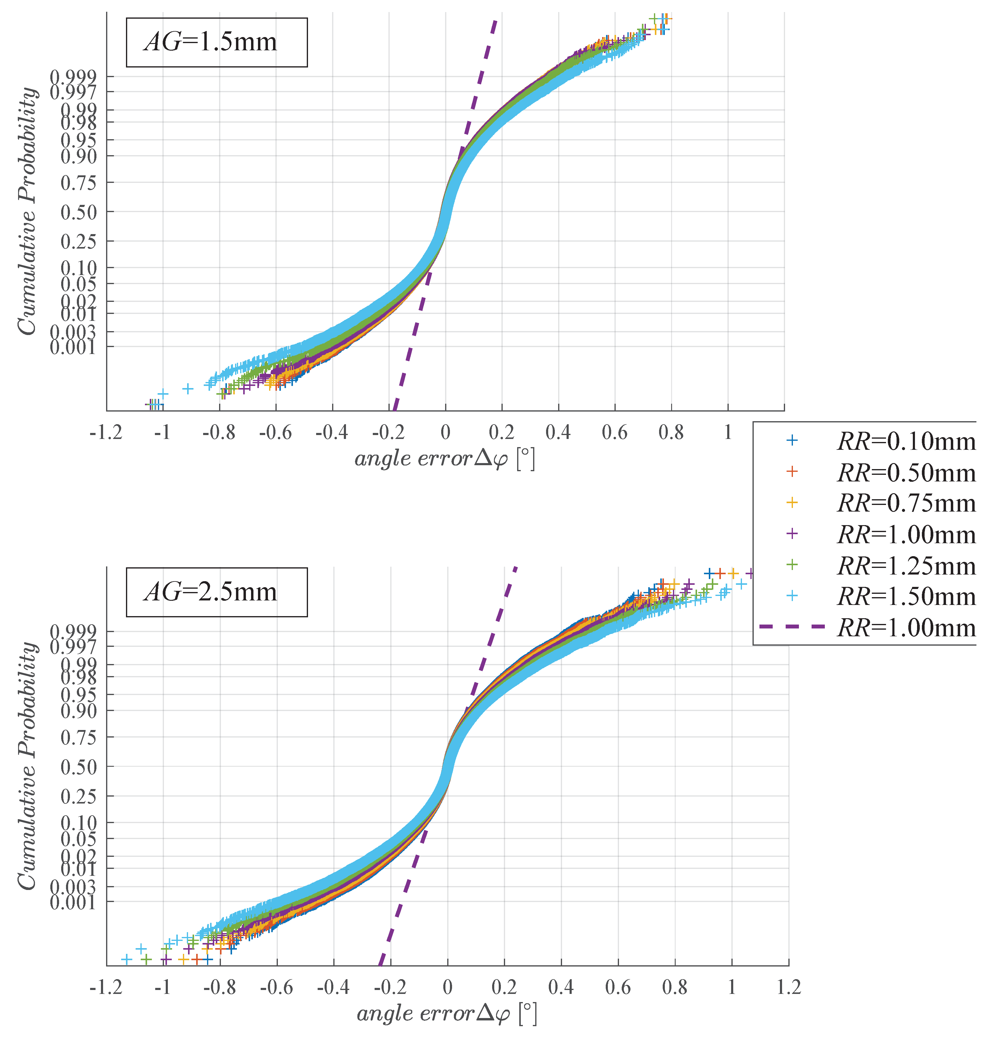
The results of the two Monte Carlo simulations for 1.5 and 2.5 mm air gaps are depicted in Figure 3 as normal probability plots. All distributions of angle errors relate to an angular position, φ = 33.75 ; however, the distributions are identical at any other rotational position φ . In this plot, a Gaussian distribution appears as a straight ascending line through the median, and its slope is determined by the interquartile range of the distribution. We plotted one such Gaussian distribution with standard deviation equal to the one of the Monte Carlo results for R R = 1.0 mm . Obviously, there is a striking difference between the Monte Carlo results and the approximated Gaussian distribution: the Gaussian distribution underestimates the 99.9 % percentile by more than three times (Figure 3).
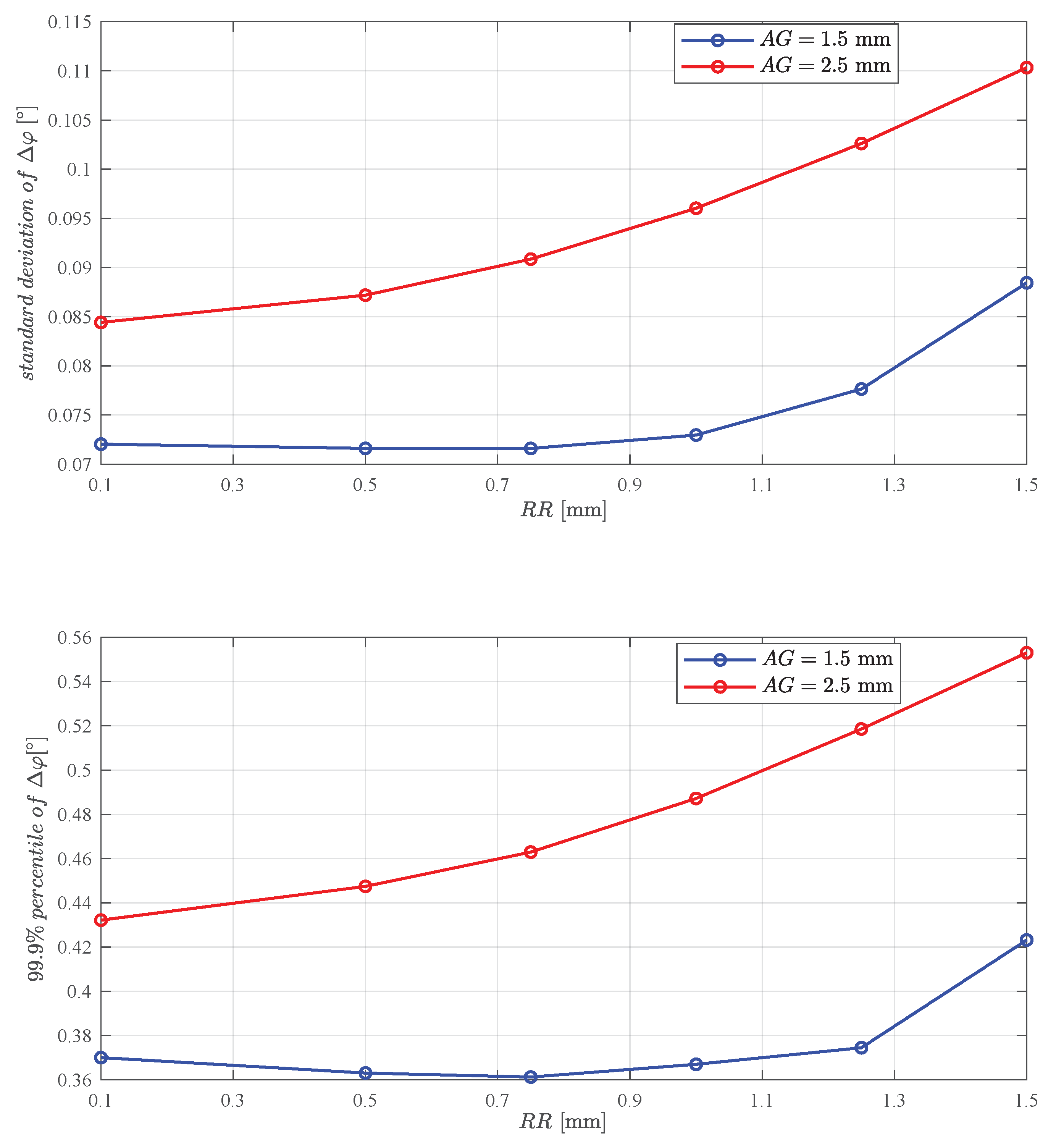
Figure 4 shows the standard deviation and the 99.9 % percentiles versus RR for the data of Figure 3. Apparently, the angle error increases only slightly with the reading radius, especially near the optimum air gap of 1.5 mm. (Compare with Figure 6.) It appears that the reading radius should at least be smaller than one third of the magnet radius ( R R < D / 6 ).

5. Discussion

The results of the Monte Carlo simulations in Figure 3 and Figure 4 led us to the following conclusions.
  • The distribution of Δ φ is clearly non-Gaussian: The angle errors of rare outliers are much bigger than one would predict with a Gaussian. Non-Gaussian error distributions have also been reported for MEMS based inclinometers by [23].
  • A variation of the reading radius has less influence on Δ φ than assembly tolerances.
  • Typical angle errors (= standard deviation) and rare outliers ( = 99.9 % percentiles) are similarly affected by R R , whereby small R R give slightly smaller angle errors.
With the analytical theory presented in [13], we can show why the distribution of angle errors has such a long tail. In [13], this angle error was expressed as a Taylor series in powers of small eccentricities and tilts (Appendix B lists assembly parameters defined in this publication and equivalent ones defined in [13]):
Δ φ = 3 4 δ M 2 s i n ( 2 η M ) + 3 4 δ S 2 s i n ( 2 ( η M + η S + φ ) ) + δ M δ S ( s i n ( η S + φ ) + 3 s i n ( η M ) c o s ( η M + η S + φ ) ) γ S + { ( δ M c o s ( η M ) + δ S c o s ( η M + η S + φ ) ) + ( y M + x S 2 + y S 2 s i n ( η M + a r c t a n 2 ( x S , y S ) + φ ) + δ M z S s i n ( η M ) ) + 1 4 ( δ M 2 z S s i n ( 2 η M ) + δ M x M 2 + y M 2 s i n ( η M + a r c t a n 2 ( x M , y M ) ) + δ M x S 2 + y S 2 s i n ( 2 η M + a r c t a n 2 ( x S , y S ) + φ ) + δ M z S δ S s i n ( 2 η M + η S + φ ) + x M 2 + y M 2 δ S s i n ( η M + a r c t a n 2 ( x M , y M ) + η S + φ ) + x S 2 + y S 2 δ S s i n ( 2 η M + a r c t a n 2 ( x S , y S ) + η S + 2 φ ) ) } T ˜ a x i a l + 1 8 { 2 x M y M + ( x S 2 + y S 2 ) s i n ( 2 ( η M + a r c t a n 2 ( x S , y S ) + φ ) ) + δ M 2 z S 2 s i n ( 2 η M ) + 2 δ M z S x M 2 + y M 2 s i n ( η M + a r c t a n 2 ( x M , y M ) ) + 2 δ M z S x S 2 + y S 2 s i n ( 2 η M + a r c t a n 2 ( x S , y S ) + φ ) + 2 x M 2 + y M 2 x S 2 + y S 2 s i n ( η M + a r c t a n 2 ( x S , y S ) + a r c t a n 2 ( x M , y M ) + φ ) } E ˜ a x i a l
with the tilt shape function of the magnet:
T ˜ a x i a l = lim y 0 1 B z ( x = 0 , y , z S + z M ) B z ( x = 0 , y , z S + z M ) z
and the eccentricity shape function of the magnet:
E ˜ a x i a l = lim y 0 1 B z ( x = 0 , y , z S + z M ) 2 B z ( x = 0 , y , z S + z M ) z 2
whereby the dipole moment of the magnet points is in the y-direction. In Appendix C, we give these shape functions homogeneously magnetized for cylindrical magnets. In Equation (25), there are no linear terms of placement tolerance parameters. This is due to the symmetry of the arrangement: in the ideal case the Hall plates are located symmetrically around the rotation axis. Therefore, all first-order terms in the angle error cancel out. The dominant lowest order error terms are of second order: the angle error rises with the second power of eccentricities and tilts. The important point is that there are also mixed 2nd order terms, such as the product of eccentricity of the magnet times tilt of magnet or the eccentricity of magnet times the eccentricity of the sensor. These mixed error terms have an important consequence: the total error is more than the sum of individual errors.
Example 1.
If a 1st system is perfectly accurate except for an eccentricity of the magnet, the angle error is
Δ φ 1 = E ˜ a x i a l 8 2 x M y M
If a 2nd system is perfectly accurate except for an eccentricity of the sensor, the angle error is
Δ φ 2 = E ˜ a x i a l 8 ( x S 2 + y S 2 ) s i n ( 2 φ + 2 a r c t a n 2 ( x S , y S ) )
However, if a 3rd system is perfectly accurate except for the eccentricities of the magnet and sensor, the angle error is
Δ φ 3 = Δ φ 1 + Δ φ 2 + E ˜ a x i a l 8 2 x M 2 + y M 2 x S 2 + y S 2 s i n ( φ + a r c t a n 2 ( x S , y S ) + a r c t a n 2 ( x M , y M ) )
The angle error of the 1st system comprises one term and the error of the 2nd system also comprises one term; however, the error of the 3rd system comprises not just two terms, but three terms. The 3rd term is proportional to the product of eccentricities of sensor and magnet. Therefore, the distribution of Δ φ 3 is wider than the statistical sum of Δ φ 1 and Δ φ 2 . For x M = y M = 0.3 mm, x S = 0.2 mm, y S = 0.1 mm, and E ˜ a x i a l = 35000 m 2 , it follows that Δ φ 1 = 0.045 , Δ φ 2 = 0.016 , and Δ φ 3 = 0.109 .
The absence of 1st order error terms means that the typical angle error is small. If a typical tilt occurs, it gives an angle error, which is proportional to the square of the small tilt.
Only in rare cases are several ones of the assembly tolerance parameters large. However, once this rare event happens, it gives a much bigger error, because the total angle error is more than the sum of individual errors for each misplacement parameter; in addition, we have to add all mixed error terms, which gives a larger total error.
With the following shorthand notation,
e M worst case angle error Δ φ if only the magnet is placed eccentrically
e S worst case angle error Δ φ if only the sensor is placed eccentrically
t M worst case angle error Δ φ if only the magnet is tilted
t S worst case angle error Δ φ if only the sensor is tilted
the total worst case angle error is given by
( e M + e S + t M + t S ) 2 = e M + e S + t M + t S + 2 ( e M e S + e M t M + e M t S + e S t M + e S t S + t M t S )
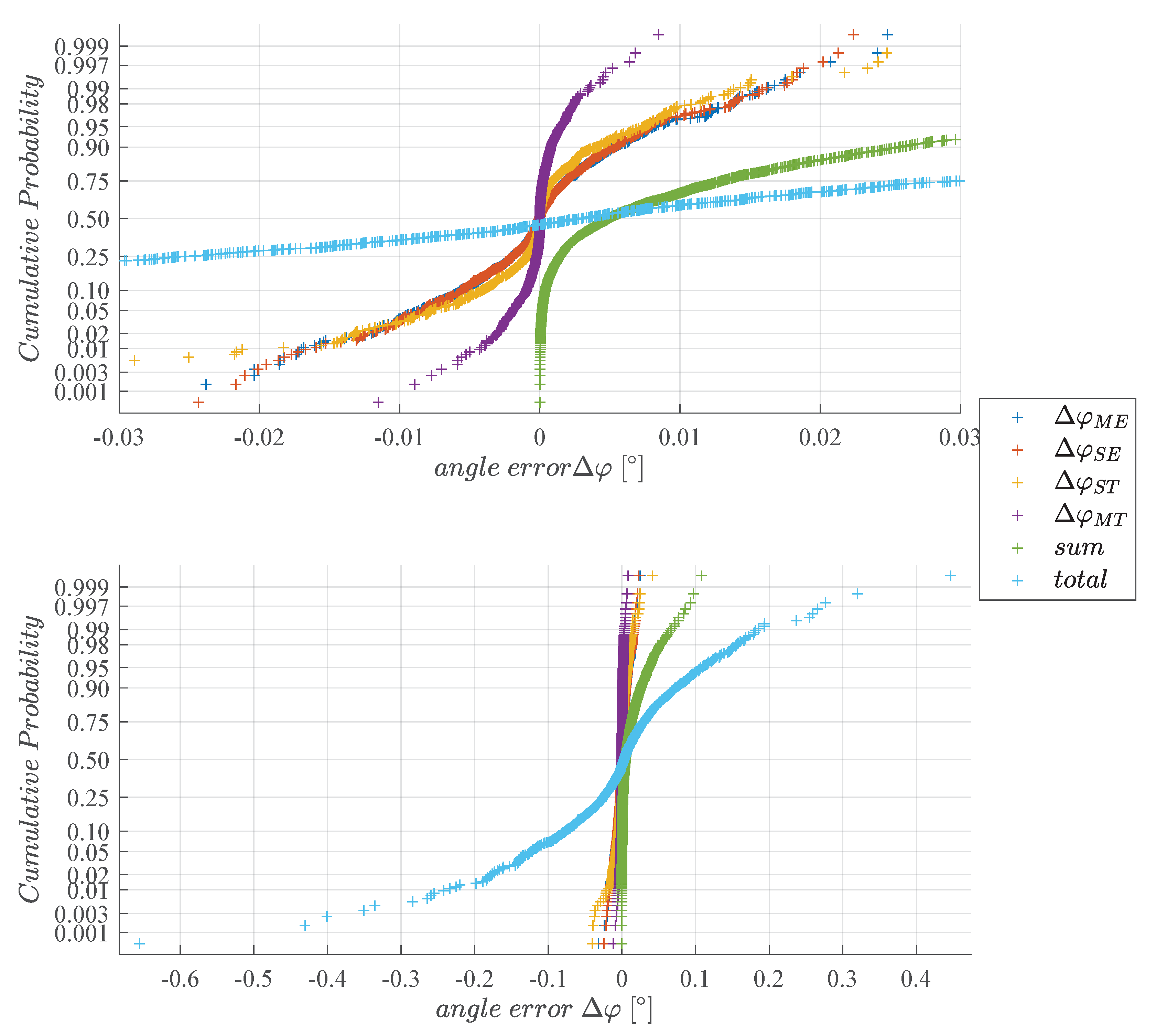
We clearly see that a single assembly parameter gives only a single term in the 1st line; however, all four assembly parameters give 10 error terms, sic of which are mixed errors. It is obvious that in the rare cases, when all four assembly parameters are large, we will end up with a much larger total error due to the six mixed error terms. This is also verified numerically in Figure 5.
According to the central limit theorem of probability theory, the sum of many Gaussian-distributed stochastic variables is again Gaussian-distributed. Yet, the angle error is the square of the sum of several Gaussian-distributed stochastic variables, and this leads to a long tail in the distribution function.
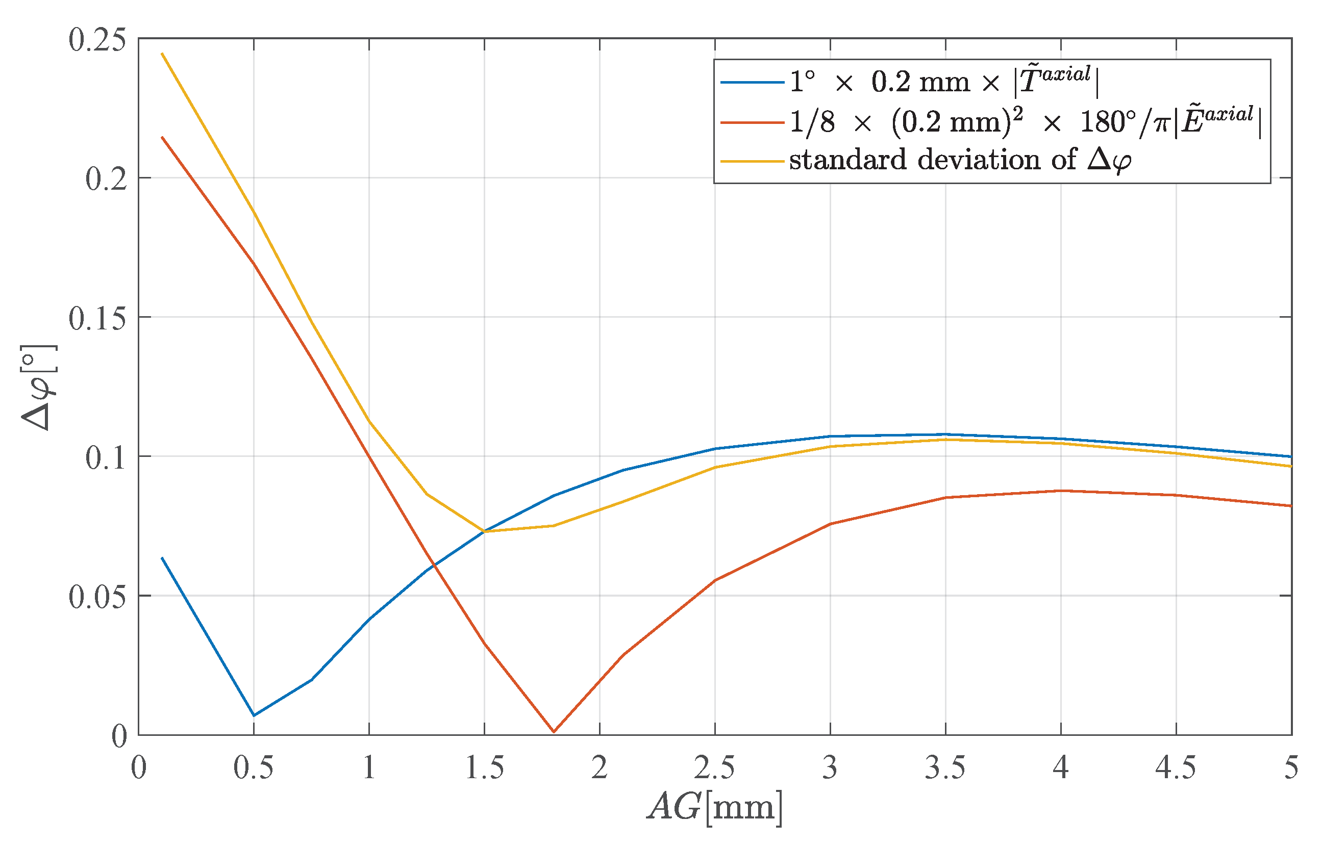
The angle error in Equation (25) consists of three parts: the first part is proportional to T ˜ a x i a l , the second part is proportional to E ˜ a x i a l , and the third comprises the remainder. The remainder comprises only tilts, not eccentricities, and it gives notably smaller values than the first two parts. If the magnet produces a homogeneous field gradient (that means d B z / d y does not vary in space), both shape functions vanish: T ˜ a x i a l = 0 and E ˜ a x i a l = 0 . In the optimization of an axial field gradient angle sensor system, one looks for magnets with vanishing shape functions. For simple magnet shapes like short cylinders, it turns out that both shape functions have a zero, yet at different air gaps. The tilt shape function vanishes at smaller air gaps than the eccentricity shape function. Due to the statistical superposition of T ˜ a x i a l terms and E ˜ a x i a l terms in the angle error, the total error has a relative minimum versus air gap for air gaps between both zeros. The exact location of the minimum depends on the relative magnitudes of the T ˜ a x i a l - and E ˜ a x i a l -terms. This is shown in Figure 6, where we plot the standard deviation of Δ φ versus AG for R R = 1 mm. In the same plot, we added an exemplary tilt error term, 1 × 0.2 mm x | T ˜ a x i a l | , and an exemplary eccentricity error term, 1 / 8 × ( 0.2 mm ) 2 × 180 / π | E ˜ a x i a l | .
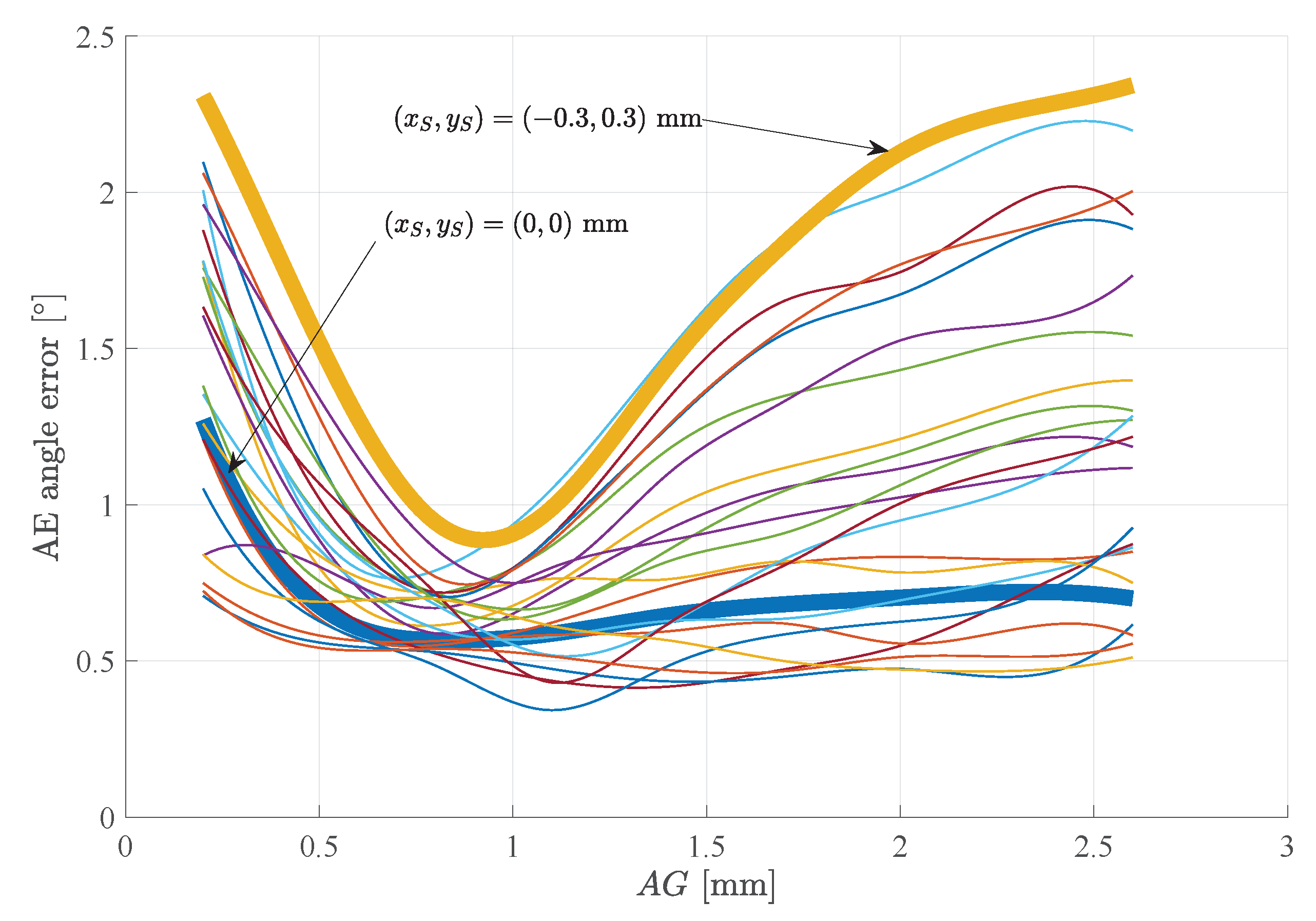
Experiments conducted on a single test chip (with R R = 1 mm) prove the statements above. Figure 7 shows the angle error versus air gap, whereby each curve was measured for a different sensor eccentricity. The sensor eccentricity x S and y S was changed in the range of [ 0.3 , 0.3 ] mm by mounting the sensor on a translation stage. The sensor tilt was nominally zero but we could not avoid possible tilts of the sensor chip inside the sensor package (up to 2 ). Also, the magnet was mounted as perfectly as possible, but again here we cannot exclude that there might have been small magnet eccentricities (up to 0.1 mm), small tilts of the magnet (up to 2 ), and small tilts of the magnetization inside the magnet (up to 3 ). However, all these unavoidable small assembly tolerances were constant for all curves, because we used a single chip and we did not change the mounting of the chip on the translation stage during the experiment, so that only the sensor eccentricity was changed via the translation stage. The measured AE angle error is defined as half the difference of maximum and minimum angle error in a 360 rotation: AE=[max ( Δ φ ) − min ( Δ φ ) ] /2. The remaining error results from unavoidable sensor tilt, magnet tilt, and magnet eccentricity, as well as errors generated in the signal processing path of this non calibrated part. Note that all curves were measured with the same chip and magnet with constant tilts and magnet eccentricity—only the sensor eccentricity was changed. The highlighted curves show the typical A G dependency from Figure 6.
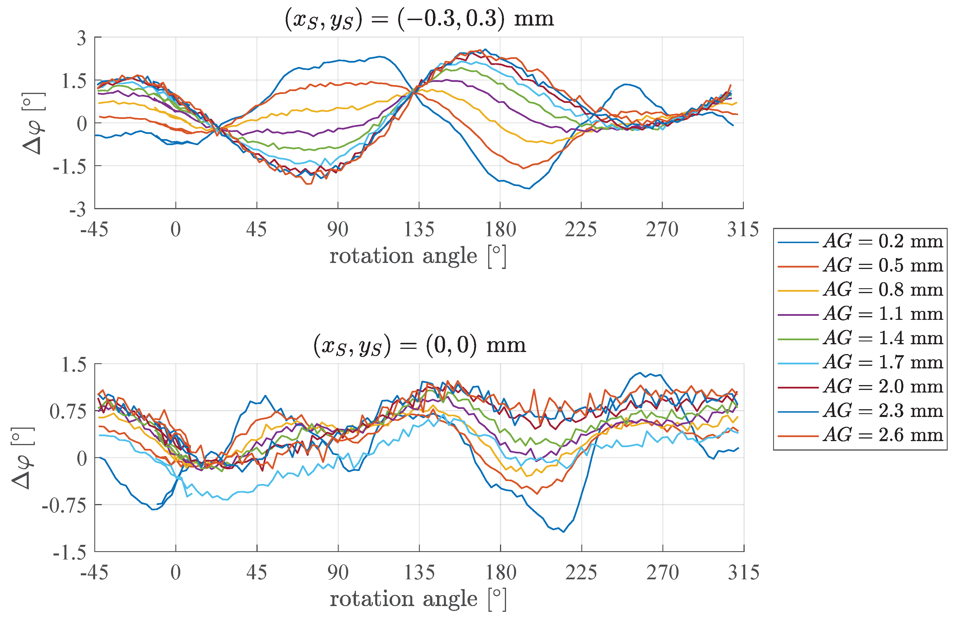
The angle error Δ φ versus rotation angle for the two bold curves (yellow, blue) in Figure 7 is shown explicitly in Figure 8. The angle error curves show one pattern at large air gaps of A G > 1.1 mm and a different pattern at small air gaps of A G 0.5 mm (compare this with the zeros of T ˜ a x i a l and E ˜ a x i a l in Figure 6). T ˜ a x i a l is dominating the error contribution for small A G , whereas E ˜ a x i a l is the dominating error contributor for larger A G . The curves for A G = 0.2 mm should be similar in both plots (as the tilts were not changed), and their respective minima and maxima are roughly at the same angle. The deviations between the two curves result from the contribution of E ˜ a x i a l .

6. Conclusions

In summary, we show that assembly tolerances have a significant impact on gradient magnetic angle sensors. Thereby, the statistical distribution of angle errors shows significantly larger errors of rare outliers than one would predict with a Gaussian distribution. The reason for the non-Gaussian distribution of angle errors is the symmetry of the sensor arrangement, which cancels out linear error terms and leaves second-order error terms. Typical errors (=standard deviation of errors) are below 0.1 and 99.9 % percentiles are five times larger. Judicious choice of magnet and air gap can reduce the angle error further. Within reasonable limits, the sensor layout (reading radius being smaller than one sixth of the magnet diameter) has much less effect on the angle error than the shape functions of the magnet.

Author Contributions

The mathematical model and the graphs were created by S.E. The experiments were conducted by M.H. All other authors contributed equally. All authors read and approved the final manuscript.

Funding

This research received no external funding.

Conflicts of Interest

The authors declare no conflicts of interest.

Abbreviations

The following abbreviations are used in this manuscript:
AEAverage Angle Error: [ m a x ( Δ φ ) - m i n ( Δ φ ) ] /2
AGAir gap
B r e m Remnant magnetization
DMagnet diameter
DoFDegree(s) of Freedom
EMIElectromagnetic Interference
HMagnet height
H c b Magnetic coercivity
GMRGiant Magnetoresistance
MDPIMultidisciplinary Digital Publishing Institute
MEMaximum Angle Error: m a x ( | m a x ( Δ φ ) | , | m i n ( Δ φ ) | )
MEMSMicroelectromechanical Systems
TMRTunnel Magnetoresistance
RRReading Radius
w.r.t.with respect to

Appendix A

The results of the model were validated against previously conducted Monte Carlo simulations in [13]. There, the magnet was a diametrically polarized disc magnet.
  • Diameter D = 10 mm
  • Height H = 2 mm
The air gap was 1 mm and the reading radius was assumed to be sufficiently small (theoretically infinitesimally small). The assembly tolerances are given in Table 2. A Monte Carlo simulation with 10,000 runs is shown in Figure 9 in [13]. There, the angle error distribution was plotted versus the ME-angle error, which is the largest absolute value of Δ φ in [ 0 , 360 ] . In [13] the author compared the ME-angle error of an axial angle sensor (as discussed in this work) to a perpendicular angle sensor. Perpendicular angle sensors are GMRs, TMRs, or Vertical Hall sensors, which respond to the magnetic field components perpendicular to the rotation axis. For this axial gradient field angle sensor we computed the distribution of angle errors with our method explained in Section 2. All parameters are identical to [13], except that we account for a reading radius of 0.1 mm. In Figure A1, we plotted the original data of [13] and our own data: both curves are fairly similar.
Figure A1. Complementary Cumulative Probability Density Function (CCDF) versus ME-angle error for the approaches presented in this publication and the one presented in [13] for R R = 0.1 mm at A G = 1 mm . Magnet parameters: D = 10 mm and H = 2 mm . Assembly tolerances according to Table 2; 10,000 Monte Carlo samples taken.
Mathematics 07 00968 g0a1
The key parameters of the distributions in Figure A1 are summarized in Table A1. They match perfectly with the values reported in [13]. The relatively large angle error ( 0.1 % of all manufactured systems have an error exceeding ~ 0.8 ) is due to the fact that the magnet is not optimal for this gradient field type of angle sensors.
Table A1. Comparison of ME-angle errors extracted from the data in Figure A1.
CCDF ValueThis PublicationIn [13]
0.1 0.31 0.32
0.01 0.54 0.56
0.001 0.78 0.81

Appendix B

Table A2. Comparison of assembly parameters used in [13] with corresponding variables in this publication.
This PublicationIn [13]
α M β c o s ( α )
β M β s i n ( α )
η M = a r c t a n 2 ( α M , β M ) α
δ M β
α S λ c o s ( γ )
β S λ s i n ( γ )
η S = a r c t a n 2 ( α S , β S ) γ
δ S λ
γ S ϑ
x S ϵ x = ϵ r c o s ( χ )
y S ϵ y = ϵ r s i n ( χ )
a r c t a n 2 ( x S , y S ) χ
z S ϵ z
x M δ x = δ r c o s ( η )
y M δ y = δ r s i n ( η )
a r c t a n 2 ( x M , y M ) η
z M δ z
Remark A1.
These equivalences are valid in good approximation for small eccentricities and tilts, but the higher-order terms differ. However, the equivalences are exact in the lowest order terms of the Taylor series approximation used in [13] and therefore they are well suited for a comparison of this work with [13]. The reason for differences in higher-order terms is that this work uses a different sequential order in the coordinate transformations than [13].

Appendix C

From Figure 12a–f in [13], we get the following expressions for the shape functions of cylinder magnets with homogeneous magnetization in diametrical direction:
T ˜ a x i a l = g ( D , H , A G , H / 2 ) g ( D , H , A G , H / 2 ) b ( D , H , A G , H / 2 ) b ( D , H , A G , H / 2 )
E ˜ a x i a l = f ( D , H , A G , H / 2 ) f ( D , H , A G , H / 2 ) b ( D , H , A G , H / 2 ) b ( D , H , A G , H / 2 )
with
b ( D , H , A G , z S ) = 1 16 ( D 2 / 4 + ( A G + H / 2 z S ) 2 ) 3 / 2
f ( D , H , A G , z S ) = 6 ( 16 A G 2 D 2 + 16 A G ( H 2 z S ) + 4 ( H 2 z S ) 2 ) ( 4 A G 2 + D 2 + 4 A G ( H 2 z S ) + ( H 2 z S ) 2 ) 7 / 2
g ( D , H , A G , z S ) = 3 ( 2 A G + H 2 z S ) ( 4 A G 2 + D 2 + 4 A G ( H 2 z S ) + ( H 2 z S ) 2 ) 5 / 2
Thereby, the peak amplitude of the magnetic induction on a single Hall plate is equal to B r e m R R D 2 ( b ( D , H , A G , H / 2 ) b ( D , H , A G , H / 2 ) . Equations (A1–A5) were used to compute T ˜ a x i a l and E ˜ a x i a l in Figure 6.
These equations neglect the small recoil permeability μ r r e c o i l = B r e m / ( μ 0 * | H c b | ) of permanent magnetic materials, with B r e m being the remanence of the permanent magnet; meaning that instead of common values of μ r r e c o i l 1.1 , they assume μ r r e c o i l = 1 . The accuracy of these approximations is all the better if H / D < < 1 . However, all the reasonable magnet geometries function as good starting points for more refined investigations of shape functions with finite element simulations (FEM).
Attention: If the magnet is attached to a ferrous shaft, this will change the magnetic field and the shape functions. Then, one has to resort to FEM simulation. Moreover, in the presence of soft magnetic parts near the sensor chip, one has to take care not to wreck the robustness of the system against electromagnetic disturbances.
For more refined shapes of magnets, it is possible to make both shape functions vanish simultaneously over a wide range of air gaps [24]. This gives angle sensors that are robust against huge magnetic disturbances without ferrous shields and extremely accurate, in spite of position tolerances. If a ferrous shaft cannot be avoided, it is better to switch the strategy and use different angle sensor systems [7].

References

  1. Granig, W.; Hartmann, S.; Köppl, B. Performance and Technology Comparison of GMR versus commonly used Angle Sensor Principles for Automotive Applications. SAE Trans. 2007, 116, 29–41. [Google Scholar] [CrossRef]
  2. Granig, W.; Kolle, C.; Hammerschmidt, C.D.; Schaffer, B.; Borgschulze, R.; Reidl, C.; Zimmer, J. Integrated Gigant Magnetic Resistance based Angle Sensor. In Proceedings of the 2006 IEEE Sensors, Daegu, Korea, 22–25 October 2006; Volume 1. [Google Scholar]
  3. Granig, W.; Weinberger, M.; Reidl, C.; Bresch, M.; Strasser, M.; Pircher, G. Integrated GMR Angle Sensor for Electrical Commutated Motors including Features for Safety Critical Applications. In Proceedings of the Eurosensors XXIV, Linz, Austria, 5–8 September 2010; Volume 1. [Google Scholar]
  4. Ausserlechner, U. Inaccuracies of Giant Magneto-Resistive Angle Sensors Due to Assembly Tolerances. IEEE Trans. Magn. 2009, 45, 2165–2174. [Google Scholar] [CrossRef]
  5. Ausserlechner, U. The optimum layout for giant magnetoresistive angle sensors. IEEE Sens. J. 2010, 10, 1571–1582. [Google Scholar] [CrossRef]
  6. Ausserlechner, U. Inaccuracies of anisotropic magneto-resistance angle sensors due to assembly tolerances. IEEE Sens. J. 2012, 10, 1571–1582. [Google Scholar] [CrossRef]
  7. Slama, P.; Aichriedler, L. Hoch performante Rotorlage-Sensorik für bürstenlose E-Maschinen in Hybridantrieben. In Automobil-Sensorik: Ausgewählte Sensorprinzipien und deren automobile Anwendung; Tille, T., Ed.; Springer: Berlin/Heidelberg, Germany, 2016; pp. 233–250. [Google Scholar] [CrossRef]
  8. Metz, M.; Häberli, A.; Schneider, M.; Steiner, R.; Maier, R.; Baltes, H. Contactless Angle Measurement Using Four Hall Devices on Single Chip. In Proceedings of the International Solid State Sensors and Actuators Conference (Transducers ’97), Chicago, IL, USA, 19 June 1997; pp. 385–388. [Google Scholar]
  9. Kaulberg, T.; Bogason, G. An Angledetector based on magnetic sensing. In Proceedings of the IEEE International Symposium on Circuits and Systems—ISCAS ’94, London, UK, 30 May–2 June 1994; pp. 329–332. [Google Scholar]
  10. Kawahito, S.; Takahashi, T.; Nagano, Y.; Nakano, K. A CMOS rotary encoder system based on magnetic pattern analysis with a resolution of 10b per rotation. In Proceedings of the 2005 IEEE International Digest of Technical Papers, Solid-State Circuits Conference, San Francisco, CA, USA, 10 February 2005; pp. 240–596. [Google Scholar]
  11. Popovic, R.S.; Drljaca, P.; Schott, C.; Racz, R. A new CMOS Hall angular position sensor (Neuer CMOS-Hall-Winkelpositionssensor. Tech. Mess. Plattf. Methoden Syst. Anwendungen Messtech. 2001, 68, 286. [Google Scholar] [CrossRef]
  12. Huber, S.; Burssens, J.W.; Dupre, N.; Dubrulle, O.; Bidaux, Y.; Close, G.; Schott, C. A Gradiometric Magnetic Sensor System for Stray-Field-Immune Rotary Position Sensing in Harsh Environment. Proceedings 2018, 2, 809. [Google Scholar] [CrossRef]
  13. Ausserlechner, U. A Theory of Magnetic Angle Sensors with Hall Plates and without Fluxguides. Prog. Electromagn. Res. B 2013, 49, 77–106. [Google Scholar] [CrossRef]
  14. Francis, L.A.; Poletkin, K. Magnetic Sensors and Devices: Technologies and Applications; CRC Press: London, UK, 2017. [Google Scholar]
  15. Kamencky, P.; Horsky, P. An inductive position sensor ASIC. In Analog Circuit Design; Springer: Dordrecht, The Netherlands, 2008; pp. 33–53. [Google Scholar]
  16. Husstedt, H.; Ausserlechner, U.; Kaltenbacher, M. In-Situ Analysis of Deformation and Mechanical Stress of Packaged Silicon Dies With an Array of Hall Plates. IEEE Sens. J. 2011, 11, 2993–3000. [Google Scholar] [CrossRef]
  17. Furlani, E. A three-dimensional field solution for axially-polarized multipole discs. J. Magn. Magn. Mater. 1994, 135, 205–214. [Google Scholar] [CrossRef]
  18. Szymanski, J.E. Basic Mathematics for Electronic Engineers: Models and Applications; Taylor & Francis: London, UK, 1989; p. 154. [Google Scholar]
  19. Hanson, J. Rotations in Three, Four, and Five Dimensions. Available online: https://arxiv.org/abs/1103.5263 (accessed on 11 September 2019).
  20. James, R.C. Mathematics Dictionary; Springer Science & Business Media: Berlin, Germany, 1992; p. 424. [Google Scholar]
  21. MathWorks Inc. Matlab Online Documentation- Normrnd. Available online: https://de.mathworks.com/help/stats/normrnd.html?s_tid=doc_ta (accessed on 7 August 2019).
  22. MathWorks Inc. MATLAB Online Documentation-Rand. Available online: https://de.mathworks.com/help/matlab/ref/rand.html?s_tid=doc_ta (accessed on 7 August 2019).
  23. Schmidt, R.; O’Leary, P.; Ritt, R.; Harker, M. MEMS Based Inclinometers: Noise Characteristics and Suitable Signal Processing. In Proceedings of the 2017 IEEE International Instrumentation and Measurement Technology Conference (I2MTC), Turin, Italy, 22–25 May 2017. [Google Scholar]
  24. Ausserlechner, U. Magnet Arrangement and Sensor Device. U.S. Patent US020170241802A1, 24 August 2017. [Google Scholar]
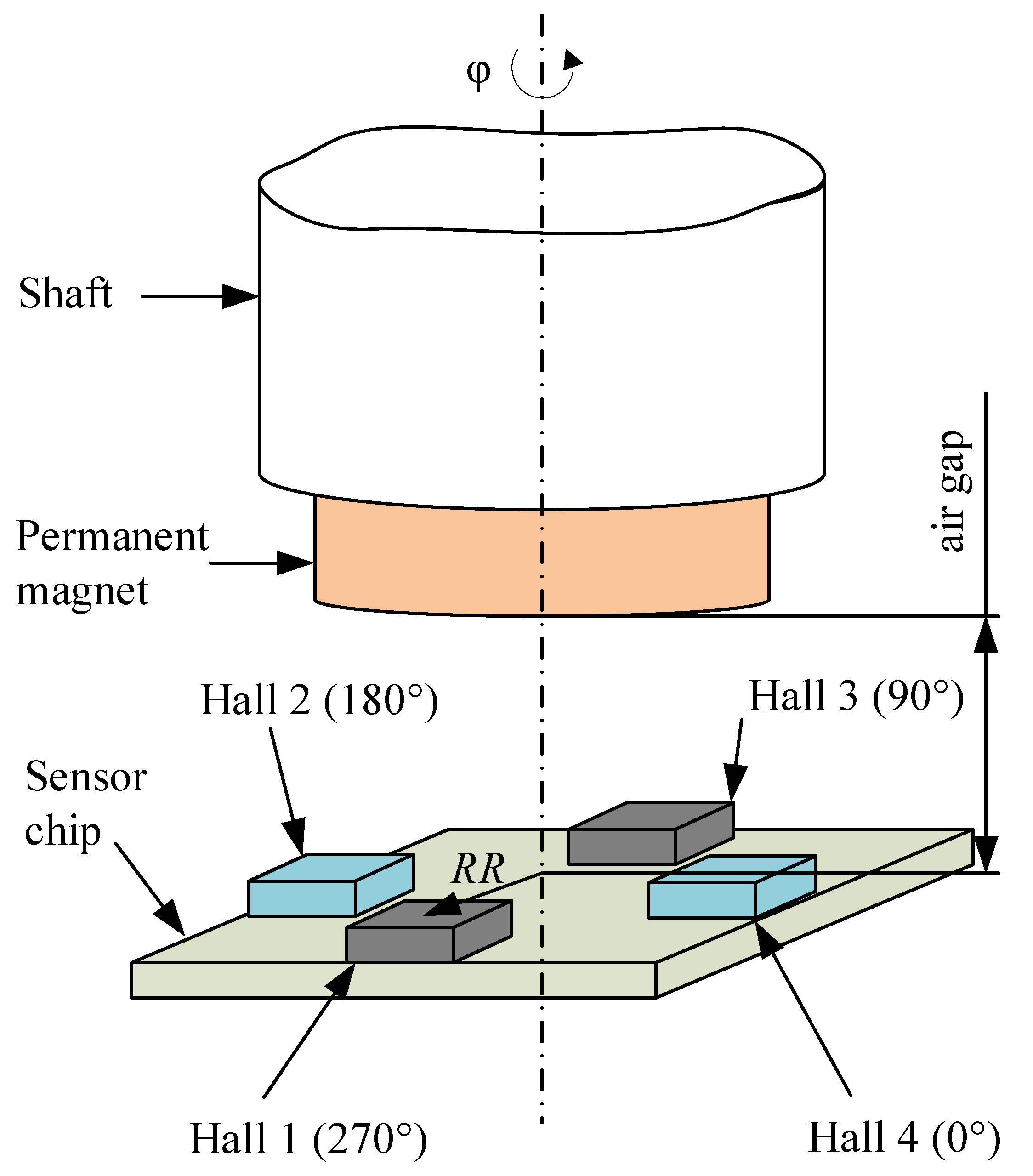
Figure 1. Schematic overview of the angle sensor system.
Mathematics 07 00968 g001
Figure 2. Schematic overview of the different coordinate systems.
Mathematics 07 00968 g002
Figure 3. Cumulative probability distribution of the angle error Δ φ at the rotation angle φ = 33.75 for various reading radii RR at an air gap A G of (a) 1.5 mm and (b) 2.5 mm . Magnet parameters: D = 6 mm and H = 2.5 mm. Assembly tolerances are according to Table 2. The dashed straight line denotes a Gaussian distribution with equal average and standard deviation. Note to legend: “+”: Monte Carlo simulation; “- - -”: Gaussian distribution with the same standard deviation as Monte Carlo simulation for R R = 1 mm; 100,000 Monte Carlo runs per configuration.
Mathematics 07 00968 g003
Figure 4. (a) Standard deviation and (b) 99.9 % percentile of Δ φ (at φ = 33.75 ) over reading radius RR for two air gaps A G . Data are from Figure 3. The ratio of percentile versus standard deviation is 5.03 and it varies about ± 3.5 % versus both A G .
Mathematics 07 00968 g004
Figure 5. Cumulative probability distribution of angle errors for assembly tolerances of Table 2. Δ φ M E = angle error for magnet eccentricity only, Δ φ S E for sensor eccentricity only, Δ φ S T for sensor tilt only, Δ φ M T for magnet tilt only, s u m = | Δ φ M E | + | Δ φ S E | + | Δ φ S T | + | Δ φ M T | , and t o t a l = real angle error if all assembly tolerances of Table 2 are simultaneously present; 1000 Monte Carlo runs conducted.
Mathematics 07 00968 g005
Figure 6. Simulated effects of statistical superposition of angle errors for a magnet as given in Section 3 with assembly tolerances according to Table 2 compared to the shape functions | T ˜ a x i a l | and | E ˜ a x i a l | .
Mathematics 07 00968 g006
Figure 7. Measured AE angle error vs. AG for a single piece of test chip with RR = 1 mm. Each curve was measured for a specific sensor eccentricity x S , y S in the range of [ 0.3 , 0.3 ] mm. All other assembly tolerances were too small to be measured, but it is very likely that they did not vanish altogether (magnet eccentricity < 0.1 mm and tilts up to a few degrees). During the experiment, the sensor was mounted only once on the translation stage, and therefore all assembly tolerances were constant, except for x S and y S . Note that the combined action of inevitable assembly tolerances and intentionally changed sensor eccentricity produces a wide variety of curves that fill up the entire area below the curve with maximum sensor eccentricity. The curve for ( x S , y S ) = ( 0 , 0 ) mm is flat for medium and large air gap, but it increases at small air gap, which is probably due to inevitable tilt errors. The curve for ( x S , y S ) = ( 0.3 , 0.3 ) mm has identical behavior at small air gap; yet, at large air gap, we clearly see the strong effect of eccentricity proportional to the rise in E ˜ a x i a l versus air gap.
Mathematics 07 00968 g007
Figure 8. Δ φ versus rotation angle for (a) ( x S , y S ) = ( 0.3 , 0.3 ) mm and (b) ( x S , y S ) = ( 0 , 0 ) mm from Figure 7. Two different patterns are detectable: T ˜ a x i a l dominates for small A G and E ˜ a x i a l dominates for large A G . Tilts and magnet eccentricity are not quantified but small and equal for all curves.
Mathematics 07 00968 g008
Table 1. Overview of degrees of freedom (DoF). DoF in bold were used in the model input.
Sensor DoFMagnet DoF
Position ( d S )Position ( d M )
x S x M
y S y M
z S z M
Orientation (w.r.t. shaft CS)Orientation (w.r.t. shaft CS)
α S α M
β S β M
γ S γ M
Table 2. Overview of assembly tolerances (eccentricities and tilts) for the sensor and magnet. Note that N ( 0 , 0.01 ) mm means an average of 0 mm and a variance of 0.01 mm 2 , which is equivalent to a standard deviation of 0.1 mm.
Sensor TolerancesMagnet Tolerances
x S N ( 0 , 0.01 ) mm x M N ( 0 , 0.01 ) mm
y S N ( 0 , 0.01 ) mm y M N ( 0 , 0.01 ) mm
z S N ( 0 , 0 ) mm z M N ( 0 , 0 ) mm
δ S N ( 0 , 1 ) δ M N ( 0 , 1 )
η S U ( 0 , 360 ) η M U ( 0 , 360 )
α S δ S c o s ( η S ) α M δ M c o s ( η M )
β S δ S s i n ( η S ) β M δ M s i n ( η M )
γ S N ( 0 , 0 ) γ M N ( 0 , 0 )