Article

Forming a Hierarchical Choquet Integral with a GA-Based Heuristic Least Square Method

1
Department of Business Administration, Chung Yuan Christian University, Taoyuan 32023, Taiwan
2
Department of Computer Science & Information Management, SooChow University, No.56 Kueiyang Street, Section 1, Taipei 100, Taiwan
*
Author to whom correspondence should be addressed.
Mathematics 2019, 7(12), 1155; https://doi.org/10.3390/math7121155
Submission received: 14 October 2019 / Revised: 18 November 2019 / Accepted: 23 November 2019 / Published: 1 December 2019

Abstract

:
Identifying the fuzzy measures of the Choquet integral model is an important component in resolving complicated multi-criteria decision-making (MCDM) problems. Previous papers solved the above problem by using various mathematical programming models and regression-based methods. However, when considering complicated MCDM problems (e.g., 10 criteria), the presence of too many parameters might result in unavailable or inconsistent solutions. While k-additive or p-symmetric measures are provided to reduce the number of fuzzy measures, they cannot prevent the problem of identifying the fuzzy measures in a high-dimension situation. Therefore, Sugeno and his colleagues proposed a hierarchical Choquet integral model to overcome the problem, but it required the partition information of the criteria, which usually cannot be obtained in practice. In this paper, we proposed a GA-based heuristic least mean-squares algorithm (HLMS) to construct the hierarchical Choquet integral and overcame the above problems. The genetic algorithm (GA) was used here to determine the input variables of the sub-Choquet integrals automatically, according to the objective of the mean square error (MSE), and calculated the fuzzy measures with the HLMS. Then, we summed these sub-Choquet integrals into the final Choquet integral for the purpose of regression or classification. In addition, we tested our method with four datasets and compared these results with the conventional Choquet integral, logit model, and neural network. On the basis of the results, the proposed model was competitive with respect to other models.

1. Introduction and Presentation of the Problem

The fuzzy integral is applied to evaluate multi-criteria decision-making (MCDM) and consider the non-additive problems between criteria [1,2]. Two well-known fuzzy integral models are widely used in the field of MCDM: The Sugeno and the Choquet integral models. Reference [3] provided the concept of the λ —measure to replace the additive requirement of classical measures, which require the properties of monotonicity and continuity. Many studies have successfully employed the Sugeno integral model in various fields, for example, data classification [4], face recognition [5], and qualitative data analysis [6]. However, these decomposable fuzzy measures cannot be super-additive for some subsets of criteria and can be sub-additive for other subsets [1]. Hence, the decomposable coefficients can only express either sub-additive or super-additive measures for the whole set of criteria and restrict the Sugeno integral model from fitting into particular MCDM problems.
However, the Choquet integral model was proposed by Choquet in 1954 [7] to represent certain kinds of interactions among criteria using the concepts of redundancy and support/synergy, which are related to the Shapley value in cooperative games and are explained in References [8,9]. The problem of identifying fuzzy measures in the Choquet integral can be considered as a mathematical programming problem to reduce the error between the predicted value and evaluated output, for example, the maximum split [10], minimum variance [11], and less constrained approach [12]. Furthermore, the heuristic least mean-squares algorithm (HLMS) was also proposed in Reference [13] to identify fuzzy measures by learning from data based on the gradient descent algorithm. However, it is hard to identify 2 n 2 fuzzy measures for a huge n criteria situation in practice.
Hence, Feference [14] proposed the concept of k-additive measures and Reference [15] proposed p-symmetric measures to reduce the number of coefficients to j = 1 k ( n j ) and [ ( | A 1 | + 1 ) ] × × [ ( | A p | + 1 ) ] 2 , where { A 1 , , A p } denotes the partition of criteria. While k-additive measures significantly reduce the complexity of identifying coefficients, determining the appropriate coefficients still overloads the ability of a decision-maker in solving practical problems (e.g., for n = 10 and k = 2, 55 coefficients should be identified). In addition, information on the partition of criteria is usually unavailable in practice.
In order to overcome the practical problem of identifying fuzzy measures in the Choquet integral model, Sugeno and his colleagues proposed the hierarchical Choquet integral models [16] to decompose the Choquet integral model into several sub-Choquet integral models based on information from the inclusion–exclusion covering (IEC) and inter-additive partition (IAP). While the hierarchical Choquet integral models significantly reduce the estimated parameters, information on the IEC or IAP is not always available. In addition, the hierarchical decomposition theorem above cannot consider possible errors when identifying fuzzy measures and might be unsuitable for use with real data.
In this paper, we use a genetic algorithm (GA) to construct hierarchical Choquet integral models to reduce the estimated fuzzy measures without information on the IEC or IAP and derive the appropriate fuzzy measures based on the mean square error between the predicted values and the ground truth data. In addition, we extend the proposed method to consider the tasks of regression and classification. Four datasets are used to compare the results between the proposed method and the conventional Choquet integral, logit model, and neural network. The experimental results show that the proposed method is competitive with respect to the criteria of the mean square error and accuracy.

2. The Choquet Integral

The Choquet integral was proposed by Choquet [7] to generalize the weighted arithmetic mean to consider complementarity or substitutivity among criteria. In this section, we give a short introduction about the theory of the fuzzy measure and the Choquet integral [1,13,17,18] as follows.
Definition 1.
Let X be a measurable set that is endowed with the properties of algebra, where is all the subsets of X. A fuzzy measure μ defined on the measurable space ( X , ) is a set functions μ : [ 0 , 1 ] , which satisfy the following properties:
(1). 
μ ( ) = 0 , μ ( X ) = 1 ;
(2). 
For all A , B , if A B then μ ( A ) μ ( B ) (monotonicity).
Definition 2.
Let ( X , , μ ) be a fuzzy measure space and f be a nonnegative measurable function. The Choquet integral of the nonnegative simple function f : X R + with respect to the fuzzy measure μ : [ 0 , 1 ] can be defined as [19]
f d μ : = i = 1 n [ f ( x i ) f ( x i 1 ) ] μ ( A i ) ,
where i indicates a permutation of the set { x i , , x n } such that 0 f ( x 1 ) f ( x 2 ) f ( x n ) and A i : = { x i , , x n } .
Since the fuzzy capacities are hard to be estimated under large criteria, many methods have been proposed to determine the fuzzy capacities without considering 2 n 2 fuzzy capacities, e.g., the M o ¨ b u i s transformation or k-additive Choquet integral.
Definition 3.
The M o ¨ b u i s transformation of μ is a set function on N defined by:
m μ ( T ) : = B T ( 1 ) | T | | B | μ ( B ) , T N .
However, any set of 2 n coefficients does not necessarily correspond to the M o ¨ b u i s transformation of a capacity on N. Hence, the boundary and monotonicity conditions must be ensured as follows [20]:
{ m ( ) = 0 , T N m ( T ) = 1 , i B T m ( B ) 0 , T N , i T .
Then, the Choquet integral of x with respect to μ is given by:
C m μ ( x ) = T N m μ ( T ) Λ x i ,
where the symbol Λ denotes the minimum operator.
Definition 4.
The Shapley index of i is defined by:
ϕ i : = K N \ i ( n | K | 1 ) ! | K | ! n ! [ μ ( K { i } ) μ ( K ) ] .
The Shapley index can be interpreted as the overall importance of i. We can also consider the concept of interaction for a pair of elements i , j N from Murofushi and Soneda (1993) as follows:
I i j : = K N \ { i , j } ( n | K | 2 ) ! | K | ! ( n 1 ) ! [ μ ( K { i , j } ) μ ( K { i } ) μ ( K { j } ) + μ ( K ) ] .
The above index can be interpreted as the positive or negative synergy between the elements.
Definition 5.
A fuzzy measure μ is said to be k-additive if its M o ¨ b u i s transformation satisfies m ( A ) = 0 for any A X such that | A | > k , and at least one subset A of X exactly k elements exists, such that m ( A ) 0 [14].
Definition 6.
A fuzzy measure μ is said to be a p-symmetric measure iff when the coarsest partition of the universal set in subsets of indifference is { A 1 , , A p } , A i , i { 1 , , p } [15].

3. Identification of Fuzzy Measures

Several methods of fuzzy measure identification for the Choquet integral have been proposed by solving a specific mathematical programming model. We introduce several popular methods as follows.

3.1. A Maximum Split Approach

Marichal and Roubens [10] proposed a linear programming model to identify fuzzy measures that can be stated as follows:
max   ε s . t . { T S t k 1 m v ( T i ) 0 ,   i N ,   S N \ i , T N 0 < t k m v ( T ) = 1 , C m v ( u ( x ) ) C m v ( u ( x ) ) δ C + ε , o t h e r   c o n s t r a i n s .
In this model, m v is the M o ¨ buis representation of a k-additive game μ on N. Note that other constraints include weights on singletons, weights on interactions, and so forth. However, if the above model contains incoherence then the solution set could be empty. A similar situation could result from incomplete information. Hence, we should add extra information to obtain an appropriate solution.

3.2. Minimum Variance Approach

The purpose of the minimum variance method [11] is to maximize the extended Havrda-Charvat entropy of Order 2. The objective function is defined as the variance of the fuzzy measures as:
M V ( m v ) : = 1 n i N S N \ i γ s ( n ) ( T S m v ( T i ) 1 n ) 2
The optimization problem takes the form of the following strictly convex quadratic program:
min M V ( m v ) s . t . { T S t k 1 m v ( T i ) 0 ,   i N ,   S N \ i , T N 0 < t k m v ( T ) = 1 , C m v ( u ( x ) ) C m v ( u ( x ) ) δ C , o t h e r   c o n s t r a i n s .
The above model is a strictly quadratic program and leads to a unique solution because of the convexity of the objective function. However, the model might be useless if the initial preferences are unavailable or give a very uneven Shapley value.

3.3. A Less Constrained Approach

This approach, which derives from the work of Meyer and Roubens [12], can be seen as a generalization of the least squares methods. The minimal preferential information that has to be provided by the decision-maker is a weak order over the available objects. The objective function is defined as:
G L S ( m v , y ) : = x [ C m v ( u ( x ) ) y ( x ) ] 2
Then, the corresponding mathematical programming model can be described as follows:
min G L S ( m v , y ) s . t . { T S t k 1 m v ( T i ) 0 ,   i N ,   S N \ i , T N 0 < t k m v ( T ) = 1 , y ( x ) ( x ) δ y , o t h e r   c o n s t r a i n s .
Here, δ y is an indifference threshold and can be considered as the desired minimal difference between the overall utilities of two objects that are viewed as significantly different by the decision-maker. However, the determination of δ y is a difficult problem since the value of δ y will affect the solution of the model.
As mentioned previously, although k-additive and p-symmetric measures can reduce the complexity of identifying fuzzy measures, a complicated MCDM problem also makes these methods infeasible. In addition, almost all mathematical programming models need extra information about the preference of the decision-makers to obtain a satisfactory result. In order to apply the Choquet integral in handling a practical regression or classification problem, a data-driven method should be considered.
The most famous algorithm for identifying the fuzzy measures between variables is the heuristic least mean-squares algorithm (HLMS) [1,13,14]. The procedures of the HLMS can be divided into two parts and are described as follows.
Step 0. Initialize the fuzzy capacities at the equilibrium state.
Step 1.1. Given a training datum (x,y), compute the error function e = C m v ( u ( x ) ) y . Let the values of the fuzzy capacities on the path be involved by x by u ( 0 ) , u ( 1 ) , , u ( n ) , where u ( 0 ) = 0 and u ( n ) = 1 .
Step 1.2. Update parameter u ( i ) to the following equation:
u n e w ( i ) = u o l d ( i ) α e e max ( x ( n i ) x ( n i 1 ) )
where α ( 0 , 1 ] is the learning rate and e max is the maximum value of the error. If y [ 0 , 1 ] , then e max = 1. The notation x ( i ) denotes the ith element of the vector x in ascending order.
Step 1.3. For every node u ( i ) , i = 1 , , n 1 , check the monotonicity relations. If e > 0 , the verification is done for lower neighbors only and if e < 0 , it is done for upper neighbors only. If a monotonicity relation is violated with u ( k ) , then u ( i ) = u ( k ) . If a monotonicity relation is violated, such as with node μ J , J X , then u ( i ) = μ J . Repeat steps 1.2 and 1.3 for i = 1 , , n 1 in the following order:
  • If e > 0 , begin by u ( 1 ) , u ( 2 ) , , u ( n 1 ) ;
  • If e < 0 , begin by u ( n 1 ) , , u ( 2 ) , u ( 1 ) .
Repeat steps 1.1 to 1.3 for all training data; this is called one iteration. Several iterations can be performed.
Step 2.1. For every node left unmodified in step 1, verify the monotonicity relations with its upper and lower neighbors. If they are not verified, modify the node as in step 1.3.
Step 2.2. For every node left unmodified in step 1, adjust its value considering the values of its upper and lower neighbors in order to have a homogeneous lattice. Let u ( i ) be the node considered:
  • Mean value of upper neighbors m ¯ ( i ) = 1 / ( n i ) upper   neighbors μ J
  • Mean value of lower neighbors m _ ( i ) = 1 / i lower   neighbors μ J
  • Minimum distance between u ( i ) and its upper (respectively lower) neighbors, denoted as d ¯ min ( i ) , (respectively d _ min ( i ) )
If m ¯ ( i ) + m _ ( i ) 2 u ( i ) > 0 , then u ( i ) is increased:
u n e w ( i ) = u o l d ( i ) + β ( m ¯ ( i ) + m _ ( i ) 2 u ( i ) ) d ¯ min ( i ) 2 ( m ¯ ( i ) + m _ ( i ) )
Otherwise u ( i ) is decreased:
u n e w ( i ) = u o l d ( i ) + β ( m ¯ ( i ) + m _ ( i ) 2 u ( i ) ) d _ min ( i ) 2 ( m ¯ ( i ) + m _ ( i ) )
and β is a constant value in ( 0 , 1 ] .
Do steps 2.1 and 2.2 for every node left unmodified in the first step. This is called one iteration; several iterations can be performed.
While the HLMS provides a rational and fast procedure to estimate fuzzy measures, it also suffers from the problem of the computational cost incurred with a high-dimensional dataset. Some papers have considered the application of a 2-additive HLMS to deal with this issue [20]. However, a 2-additive HLMS still cannot handle a high-dimensional dataset soundly by reducing the number of fuzzy measures to an acceptable amount. For example, if a dataset contains 50 variables, then the number of the fuzzy measures will be 1275.

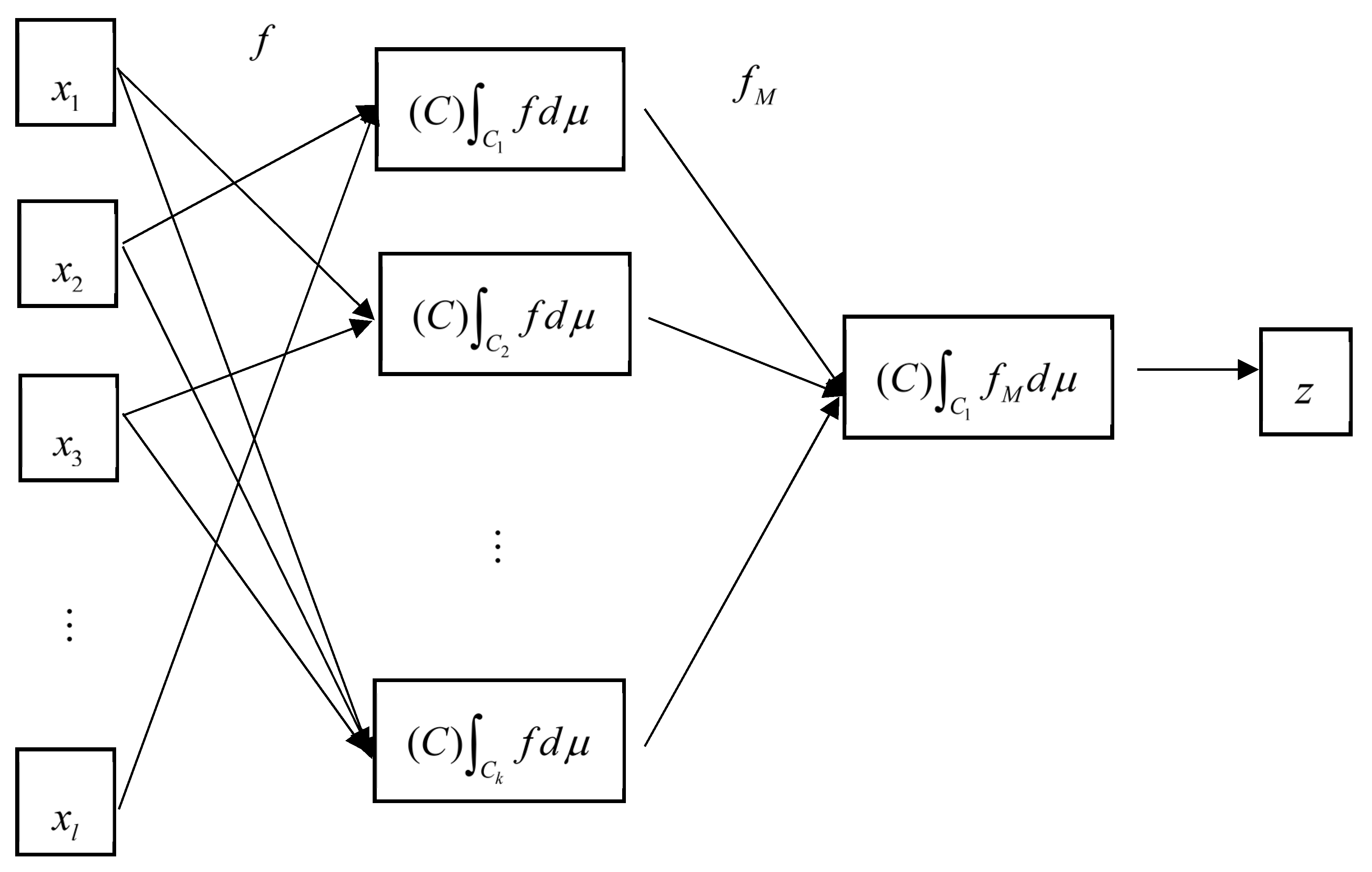
4. Hierarchical Choquet Integral

The concept of the hierarchical Choquet integral was proposed by Sugeno and his colleagues [16,21,22,23] to decompose a Choquet integral model into several sub-Choquet integral models. They gave the definitions of the inter-additive partition (IAP) and inclusion-exclusion covering (IEC) to construct the hierarchical Choquet integral.
Definition 7.
A finite measurable partition { P i } i { 1 , , n } of X is called an IAP of X if
μ ( A ) = i { 1 , , n } μ ( A P i )
for every A .
Definition 8.
A finite measurable covering { C i } i { 1 , , n } of X is called an IEC of X if
μ ( A ) = I { 1 , , n } I ( 1 ) | I | + 1 μ ( i I C i A )
for every A .
Suppose that C = { C i } i { 1 , , n } is a measurable covering, then each subalgebra S i of is defined by S i : = { C i A | A } . Let M = { μ C i ( ) } i { 1 , , n } be an n-ary class of non-monotonic fuzzy measures on S = { S i } i { 1 , , n } . The function f M on C is defined by
f M ( C i ) : = ( C ) C i f d μ C i
for every measurable function f on . Then, the hierarchical Choquet integral model is defined by the model whose input is f ( x ) on , whose output z is represented as z = ( C ) C f M d v , where v is a non-monotonic fuzzy measure on 2 C .
Then, Sugeno [16] gave the necessary and sufficient condition for an ordinary Choquet integral model and concluded that an overlapping hierarchical Choquet integral model can be hierarchically constructed by an IEC from an ordinary Choquet integral model and a separated hierarchical Choquet integral model can be hierarchically constructed by the IAP from an ordinary Choquet integral model. Hence, information on the IEC and IAP is the key to formulating the hierarchical Choquet integral. Similar to the concept of the IEC and IAP, Tzeng and Huang [24] used the idea of preference separability to construct a hierarchical Choquet integral model.
The concept of the hierarchical Choquet integral is very attractive because it can significantly reduce the number of fuzzy capacities in a model, but the key information is how to divide variables to form sub-Choquet integrals. In addition, the identification of fuzzy measures in real data usually contains errors; however, the hierarchical decomposition theorem above cannot be expected to be satisfied exactly. Furthermore, the identification of IEC, IAP, and preference-separable sets is another difficult problem that arises when dealing with realistic data.

5. GA-Based HLSM

In this paper, we considered our research structure, as shown in Figure 1. First, we considered a real dataset and represented a problem with a hierarchical Choquet integral model. Then, we used Gas to determine the linkage between the input criteria and neurons. Next, we used the HLSM to train the fuzzy measures and calculated the results of the sub-Choquet integral. Furthermore, these results were used to form another regression or classifier to complete a hierarchical Choquet integral for a chromosome. Finally, the processes continued until the stop criterion of GA was met to obtain the final result of the hierarchical Choquet integral.
In this paper, we considered the hierarchical structure, as shown in Figure 2. In Figure 2, we used genetic algorithms to determine what linkages should be generated from input variables to a sub-Choquet integral. Then, the HLSM was used to derive fuzzy measures and the results of the sub-Choquet integral. Finally, all sub-Choquet integrals were weighted to calculate the final Choquet integral and gave the predicted values.

5.1. GA

The GA was introduced by Holland [25] to mimic the natural evolution of a population by allowing solutions to reproduce chromosomes, create new offspring, and compete for survival in the next generation. In each generation, t, the fittest elements were selected to the mating pool, which was processed by three basic genetic operators for generating new offspring: Reproduction, crossover, and mutation. Based on the principle of the survival of the fittest, we observed that the best chromosome of a sample solution could be obtained. The power of the GA depended on its ability to search for multiple points in a parallel manner instead of a single point. Therefore, the GA could quickly find the appropriate global optimum and avoid reaching a local optimum. The purpose of using the GA in this paper was to determine the input variables required to key into a sub-Choquet integral.

5.2. The GA Procedure

String Representation

To represent the problem, each chromosome was encoded by applying binary strings l i j . The binary value of the ijth genotype (chromosome value) denotes the linkage status from the ith criterion to the jth sub-Choquet integral. Therefore, we should have nm binary strings if we have n criteria and an m sub-Choquet integral.

Population Initialization

The initial population, P(0), could be selected at random between 0 and 1. Each genotype can be initialized to describe the status of the variables from the uniform distribution in the population. Note that there is no standard method for determining the size of the initial population, P(0). Bhandari et al. [26] showed that, as the number of iterations tends to infinity, the elitist strategy of the GA will provide the optimal string for any size of the initial population, P(0).

Fitness Computation

Here, the objective was to determine the optimal fuzzy measure coefficients by determining, automatically, the HCI with the minimum error between the predicted and the actual values. Hence, the fitness computation could be defined by
A c c u r a c y = 1 1 n x [ H C m v ( u ( x ) ) y ( x ) ] 2
where n denotes the number of instances, H C m v ( u ( x ) ) denotes the value of the final HCI value, and y ( x ) denotes the ground truth class.

5.3. Genetic Operators

Selection. Using the concept of survival of the fittest from natural genetic systems, the selection operator selects chromosomes from the mating pool. Therefore, the good chromosomes get numerous copies, whereas the bad chromosomes die off. The probability of the chromosome’s selection is proportional to its fitness value in the population, which is based on the following formula
P ( x i ) = f ( x i ) j = 1 N f ( x j )
where f ( x i ) denotes the fitness value of the ith chromosome and N denotes the population size. In addition, we used the tournament selection to process the selection operator.
Crossover. The main objective of the crossover was to exchange information between two parent chromosomes and produce two new offspring for the next generation. Several crossover operators could be investigated, such as one-point, two-point, and mask-crossover operators. However, we employed the two-point crossover and set the crossover probability to be equal to 0.8. For example, if we consider three input variables and three sub-Choquet integrals, the design of the crossover here is presented in Figure 3.
The 2nd offspring chromosome can be explained as the first sub-Choquet integral consisting of the input variables x 1 , x 2 , and x 3 . The fuzzy measure coefficients are calculated among these variables.
Mutation. Mutation is a random process in which one genotype is replaced by another to generate a new chromosome. Each genotype has the probability of mutation, Pm, to undergo a mutation change from 0 to 1, and vice versa. We set the mutation probability to be 0.1 in this paper. For example, we can consider a parent and offspring chromosomes with the mutation operator, as shown in Figure 4.

5.4. Elitist Strategy and Termination Criterion

Elitist Strategy. The elitist strategy carries the fittest chromosome from the previous generation to the next generation. The advantage of the elitist strategy lies in ensuring the selection of the best chromosome and reducing the time of convergence. We set the number of elitists to four in our experiment.
Stop Criterion. The GA typically used two stop criteria: One to set up a maximum number of generations, such as 500 iterations, and the other is triggered when the chromosomes can no longer increase the fitness. We used the first criterion in this paper.

6. Numerical Experiments

In this section, we illustrate the processes of the proposed method and used four datasets to test its effectiveness by considering the regression and classification problems. The first step of the model was to set the parameters of the GA as follows.

6.1. Parameters of GA

For the parameters of the GA in this paper, we employed the following settings, as shown in Table 1.
In addition, we set two fitness functions for the experiments to consider the tasks of regression and classification, respectively, as follows:
f i t n e s s   1 = 1 n x [ C m v ( u ( x ) ) y ( x ) ] 2 λ j = 1 J ( # ( S C j ) k j ) 2
f i t n e s s   2 = 1 n ( T P + T N ) λ j = 1 J ( # ( S C j ) k j ) 2
The first term of fitness 1 denotes the mean square error, TP and TN are the numbers of true positive and negative amounts, n is the number of instances, y ( x ) is the ground truth value, # ( S C j ) denotes the number of input variables in the jth sub-Choquet integral, k denotes the desired number of input variables in the jth sub-Choquet integral, and λ is the penalty parameter.

6.2. Dataset Description

In these experiments, we considered four datasets to demonstrate the proposed method and compared the results with the conventional Choquet integral and classification models—the logit model and neural network. The first two datasets were used for the task of regression and the last two datasets were used for the task of classification. These datasets are described as follows.
The simulated dataset is an artificial dataset that randomly generates positive integers between one and ten. It contains 200 instances and 10 independent variables with one response variable.
The add10 dataset is an artificial dataset gathered from the Delve datasets. It contains 9792 instances and 10 independent variables generated from a uniform distribution between 0 and 1, and one response variable generated by a nonlinear function, which is composed of the first five independent variables. Here, we sampled 500 instances in order to prevent the problem of an expensive computation cost.
The ILPD (Indian liver patient dataset) dataset contains 10 variables that describe the patients’ age, gender, total bilirubin, direct bilirubin, and so forth, and the response variable is whether the patients are liver patients or non-liver patients. There are 583 instances comprised of 416 liver patients and 167 non-liver patient records. Here, we only deleted one discrete variable, gender, to retain the remaining nine continuous variables.
The cancer dataset was derived from the University of Wisconsin to record diagnostic breast cancer data. It contains 699 instances and 10 variables, including clump thickness, the uniformity of the cell size, marginal adhesion, and so forth, and all variables are measured with one to ten scores. The response variable is binary (0 for benign and 1 for malignant).

6.3. Experiment Results

We can demonstrate the processes of the proposed method as follows. Take the simulated dataset for example. First, we set the number of the sub-Choquet integral as two and each sub-Choquet contains five input variables. Then, we ran the GA, as described previously, to select the appropriate input variables for each sub-Choquet integral and calculated the weighted Choquet integral to predict the value of the response variable, as shown in Figure 5 and Figure 6.
Finally, we could obtain the input variables for each sub-Choquet integral and the weight of the Choquet integral, which is the sum of the two sub-Choquet integrals under the fitness of the mean square error. The results of the Mobius capacity and fitness could be derived, as shown in Table 2.
We could set different hierarchical Choquet integral (HCI) models to calculate the mean square error and compared it with the conventional Choquet integral, as shown in Table 3.
It can be seen that the HCI provided a more flexible way to reduce the estimated fuzzy capacities of the variables and outperformance than the conventional Choquet integral used to deal with the task of resolving regression problems.
Next, we could replace our regression model with a classifier to process the task of the classification problem. Here, we considered two popular classifiers, the logit model and multi-layer perceptron (MLP), to serve as the benchmark of the proposed method. Note that we set the MLP model as a three-tier network (i.e., one input layer, one hidden layer with three neurons, and one output layer), and the activation function is the sigmoid function. In addition, we also set three HCI models for each dataset to show the variety of the model’s accuracy. The results of the experiment could be presented, as shown in Table 4.
From Table 4, it can be seen that, with the release of the number of variables, the accuracy of the model was getting higher. In addition, the proposed method was still competitive with respect to that of the logit model and MLP. Furthermore, the most attractive point of the proposed method is its explain-ability of the model, compared with that of the MLP, which can only be considered as a block box.

7. Discussion

The identification of fuzzy measures played an important role in facilitating the Choquet integral’s ability to handle realistic problems. While the Choquet integral has been used for different fields of MCDM, such as feature selection [20], image detection [27], and prediction [28], the huge number of estimated fuzzy measures usually hinders its possible applications. Even though the concept of k-additive, usually 2-additive, fuzzy measures has been proposed to reduce the number of fuzzy measures, it is still a problem when considering really high-dimensional data.
In this paper, we considered a hierarchical Choquet integral to solve the problem of identifying fuzzy measures with high-dimensional data. The main difference between the proposed method and Sugeno and Fujimoto [16] or Tzeng and Huang [24] methods is that, without advance information on the sub-Choquet integrals, the variables will be assigned to the specific sub-Choquet integrals according to the best result of the offspring, with respect to the criterion of MSE or accuracy.
In addition, we compared the proposed method with other conventional approaches by considering the tasks of regression and classification. On the basis of the experimental results, it can be seen that the proposed method is competitive with respect to the other models. In addition, the experimental results also indicated the importance of variable selection in the Choquet integral. That is, not all variables put into the model show the best results.
Finally, the advantages of the proposed method are described as follows. First, the proposed method provides flexibility for a decision-maker to determine how many inputs to add into a sub-Choquet integral. This will be useful when we consider very high-dimensional data. Second, we proposed a data-driven approach to automatically select the most appropriate variables in a sub-Choquet integral. Third, we can simply add a regression or classifier behind the HLMS to consider the task of regression or classification.

8. Conclusions

In this paper, we developed a method to construct the hierarchical Choquet integral by using the GA. The major advantage of the HCI was the reduction in the number of estimated fuzzy capacities between variables. Hence, the proposed method is very suitable for dealing with realistic datasets and enables the Choquet integral to be used for more complicated applications, including the tasks of regression and classification. In addition, the results of the experiments also indicated that the proposed method outperforms the conventional Choquet integral and classifier, namely the logit model and MLP.

Author Contributions

Data curation, C.-Y.C.; Methodology, J.-J.H.; Writing—review & editing, C.-Y.C. and J.-J.H.

Funding

No funding was received.

Conflicts of Interest

The authors declare no conflict of interest.

References

  1. Grabisch, M. Fuzzy integral in multicriteria decision making. Fuzzy Set. Syst. 1995, 69, 279–298. [Google Scholar] [CrossRef]
  2. Hillier, F. Evaluation and Decision Models: A Critical Perspective; Kluwer Academic Publishers: Boston, MA, USA, 2001. [Google Scholar]
  3. Sugeno, M. Theory of Fuzzy Integrals and Its Applications. Ph.D. Thesis, Tokyo Institute of Technology, Tokyo, Japan, 1974. [Google Scholar]
  4. Zhai, J.; Zang, L.; Zhou, Z. Ensemble dropout extreme learning machine via fuzzy integral for data classification. Neurocomputing 2018, 275, 1043–1052. [Google Scholar] [CrossRef]
  5. Karczmarek, P.; Kiersztyn, A.; Pedrycz, W. On developing Sugeno fuzzy measure densities in problems of face recognition. Int. J. Mach. Intell. Sens. Signal Process. 2017, 2, 80–96. [Google Scholar]
  6. Couceiro, M.; Dubois, D.; Prade, H.; Rico, A. Enhancing the expressive power of Sugeno integrals for qualitative data analysis. In Advances in Fuzzy Logic and Technology 2017; Springer: Berlin/Heidelberg, Germany, 2017; pp. 534–547. [Google Scholar]
  7. Choquet, G. Theory of capacities. Ann. de l’institut Fourier 1954, 5, 131–295. [Google Scholar] [CrossRef]
  8. Murofushi, T. A technique for reading fuzzy measures (I): The Shapley value with respect to a fuzzy measure. In Proceedings of the 2nd Fuzzy Workshop, Heeze, The Netherland, 4–5 June 2018; pp. 39–48. [Google Scholar]
  9. Murofushi, T.; Soneda, S. Techniques for reading fuzzy measures (III): Interaction index. In Proceedings of the 9th Fuzzy System Symposium, Sapporo, Japan, 24–26 November 1993; pp. 693–696. [Google Scholar]
  10. Marichal, J.-L.; Roubens, M. Determination of weights of interacting criteria from a reference set. Eur. J. Oper. Res. 2000, 124, 641–650. [Google Scholar] [CrossRef]
  11. Kojadinovic, I. Minimum variance capacity identification. Eur. J. Oper. Res. 2007, 177, 498–514. [Google Scholar] [CrossRef]
  12. Meyer, P.; Roubens, M. Choice, ranking and sorting in fuzzy multiple criteria decision aid. In Multiple Criteria Decision Analysis: State of the Art Surveys; Springer: Berlin/Heidelberg, Germany, 2005; pp. 471–503. [Google Scholar]
  13. Grabisch, M. The application of fuzzy integrals in multicriteria decision making. Eur. J. Oper. Res. 1996, 89, 445–456. [Google Scholar] [CrossRef]
  14. Grabisch, M. K-order additive discrete fuzzy measures and their representation. Fuzzy Sets Syst. 1997, 92, 167–189. [Google Scholar] [CrossRef]
  15. Miranda, P.; Grabisch, M.; Gil, P. p-Symmetric fuzzy measures. Int. J. Unc. Fuzz. Knowl. Based Syst. 2002, 10, 105–123. [Google Scholar] [CrossRef]
  16. Sugeno, M.; Fujimoto, K.; Murofushi, T. A hierarchical decomposition of Choquet integral model. Int. J. Unc. Fuzz. Knowl. Based Syst. 1995, 3, 1–15. [Google Scholar] [CrossRef]
  17. Hougaard, J.L.; Keiding, H. Representation of preferences on fuzzy measures by a fuzzy integral. Math. Soc. Sci. 1996, 31, 1–17. [Google Scholar] [CrossRef]
  18. Mesiar, R. Fuzzy measures and integrals. Fuzzy Set. Syst. 2005, 156, 365–370. [Google Scholar] [CrossRef]
  19. Ishii, K.; Sugeno, M. A model of human evaluation process using fuzzy measure. Int. J. Man-Mach. Stud. 1985, 22, 19–38. [Google Scholar] [CrossRef]
  20. Miranda, P.; Grabisch, M. Optimization issues for fuzzy measures. Int. J. Unc. Fuzz. Knowl. Based Syst. 1999, 7, 545–560. [Google Scholar] [CrossRef]
  21. Murofushi, T.; Sugeno, M.; Fujimoto, K. Separated hierarchical decomposition of the Choquet integral. Int. J. Unc. Fuzz. Knowl. Based Syst. 1997, 5, 563–585. [Google Scholar] [CrossRef]
  22. Fujimoto, K.; Murofushi, T.; Sugeno, M. Canonical hierarchical decomposition of Choquet integral over finite set with respect to null additive fuzzy measure. Int. J. Unc. Fuzz. Knowl. Based Syst. 1998, 6, 345–363. [Google Scholar] [CrossRef]
  23. Murofushi, T.; Fujimoto, K.; Sugeno, M. Canonical separated hierarchical decomposition of the Choquet integral over a finite set. Int. J. Unc. Fuzz. Knowl. Based Syst. 1998, 6, 257–272. [Google Scholar] [CrossRef]
  24. Tzeng, G.-H.; Huang, J.-J. Multiple Attribute Decision Making: Methods and Applications; Chapman and Hall/CRC: Boca Raton, FL, USA, 2011. [Google Scholar]
  25. Holland, J.H. Adaptation in Natural and Artificial Systems; University of Michigan: Ann Arbor, MI, USA, 1975; Volume 1, p. 975. [Google Scholar]
  26. Bhandari, D.; Murthy, C.; Pal, S.K. Genetic algorithm with elitist model and its convergence. Int. J. Pattern Recognit. Artif. Intell. 1996, 10, 731–747. [Google Scholar] [CrossRef]
  27. El Baf, F.; Bouwmans, T.; Vachon, B. Fuzzy integral for moving object detection. In Proceedings of the 2008 IEEE International Conference on Fuzzy Systems (IEEE World Congress on Computational Intelligence), Hong Kong, China, 1–6 June 2008; pp. 1729–1736. [Google Scholar]
  28. Yang, R.; Wang, Z.; Heng, P.A.; Leung, K.S. Fuzzified Choquet integral with a fuzzy-valued integrand and its application on temperature prediction. IEEE Trans. Syst. Man Cybern. Part B (Cybern.) 2008, 38, 367–380. [Google Scholar] [CrossRef] [PubMed]
Figure 1. The research structure of this paper.
Mathematics 07 01155 g001
Figure 2. Hierarchical Choquet Integral.
Mathematics 07 01155 g002
Figure 3. A two-point crossover operator.
Mathematics 07 01155 g003
Figure 4. The mutation operator.
Mathematics 07 01155 g004
Figure 5. The convergent process of GA.
Mathematics 07 01155 g005
Figure 6. Network structure of a hierarchical Choquet integral.
Mathematics 07 01155 g006
Table 1. Parameter settings of GA.
ParametersValue
Gene typeBinary
Population size50
Number of generations30
Elitism4
Crossover probability0.8
Mutation probability0.2
Table 2. The Mobius capacities and results of the parameters of the example.
2-Additive and 2 Sub-Choquet Integral
Each Sub-Choquet Integral Contains 5 Features
MSE = 2.359
Sub-Choquet 1Mobius CapacitySub-Choquet 2Mobius Capacity
{1}0.1819{2}0.2885
{4}0.2550{3}0.1414
{5}0.1785{4}0.1610
{8}0.1680{6}0.1685
{9}0.1520{7}0.1455
{1,4}0.1436{2,3}−0.0874
{1,5}0.0268{2,4}−0.1140
{1,8}−0.0039{2,6}0.0326
{1,9}−0.0578{2,7}0.0542
{4,5}−0.1510{3,4}0.2016
{4,8}−0.1012{3,6}−0.0534
{4,9}0.0538{3,7}0.0413
{5,8}0.1337{4,6}0.0148
{5,9}−0.0275{4,7}−0.0239
{8,9}0.0482{6,7}0.0292
Table 3. Performance comparison between different models and datasets.
Dataset: Simulated Dataset
Model# Sub-Choquet IntegralConditionMSE
2-additive HCI25 variables for each Sub-Choquet Integral2.359
2-additive HCI26 variables for each Sub-Choquet Integral2.221
2-additive HCI2Unrestricted2.138
Choquet Integral0Unrestricted2.138
Dataset: Add10 Dataset
Model# Sub-Choquet IntegralConditionMSE
2-additive HCI24 variables for each Sub-Choquet Integral0.00767
2-additive HCI25 variables for each Sub-Choquet Integral0.00692
2-additive2Unrestricted0.00663
Choquet Integral0Unrestricted0.00692
Note: # Sub-Choquet Integral denotes the number of sub-Choquet integrals.
Table 4. The accuracy of the classification models.
DatasetsLogit ModelMLP2-Additive HCI
cancer0.96400.97100.8141 (restrict 4 variables)
0.9531 (unrestricted)
ILPD0.70740.71490.7150 (restrict 5 variables)
0.7237 (unrestricted)

