Stage-Dependent Structured Discrete-Time Models for Mosquito Population Evolution with Survivability: Solution Properties, Equilibrium Points, Oscillations, and Population Feedback Controls

Abstract

This paper relied on the investigation of the properties of the stage-structured model of coupled larvae and adult mosquito populations’ evolution when parameterized, in general, by time-varying (or stage-dependent) sequences. In particular, the investigated properties were the non-negativity of the solution under non-negative initial conditions, the boundedness of the sequence solutions under any finite non-negative initial conditions, the equilibrium points, and the convergence conditions to them in the event that the parameterizing sequences converge to finite limits. Some further properties that were investigated relied on deriving the oscillation conditions of the solutions under certain conditions of the parameterizations. The use of feedback controls to decrease the foreseen numbers of alive mosquitoes in future evolution stages is also proposed. The proposed control actions are exerted on the birth rate and/or the maximum progression rate sequences. Some illustrative examples are also given.

1. Introduction

It is well-known from the related background literature that mosquitoes undergo complete metamorphosis following a life cycle of four stages, namely, egg, pupae, larva, and adult. See, for instance, [1] for an easily comprehensible description of those stages and the duration period of each of them. Mosquitoes typically stay in an aquatic environment during the first three life stages and in an aerial environment during their adult stage. Mathematical models are useful to describe the evolution of the mosquito population. The introduction of sterile mosquitoes in the environment in order to reduce the fertility of the whole population and control their populations under acceptable levels of tolerance has been proposed in the background literature. See, for instance, [1,2,3], and some of the references therein. Also, the study of releases of sterile mosquitoes has been investigated in [4], with a Beverton–Holt type model for survivability, as well as in [5]. It is well-known that Beverton–Holt type models are very popular to study the evolution of species that reproduce by eggs, [4,6,7,8,9,10,11,12] such as birds, insects, or fish. More general difference equations which generalize those kinds of problems are studied in detail in [13,14].

The investigation of some evolution models for mosquitoes is directly linked to the evolution of some transmission diseases of host/vector type. For instance, in [5], a malaria model was studied with a stage-type evolution type of mosquitoes. See also some references therein and [12]. In [15,16,17,18,19,20,21] several epidemic models, without or with different vaccination and treatment controls of constant and feedback-type, were discussed and studied in detail. Note that, as far as our current problem at hand is concerned, it turns out that the use of programmed aerial or aquatic insecticide can also be of practical interest to control the mosquito populations as a potential alternative to the introduction of sterile mosquitoes in the habitat of wild mosquitoes. At the same time, it appears to be evident that some admissibility levels should be imposed on such controls in order to avoid intolerable ecological damage to the environment.

The paper discusses the properties of the stage-structured model of combined larvae and adult mosquito populations’ evolution when parameterized by time-varying (or stage-dependent) sequences. In particular, the investigated properties were the non-negativity of the solution under non-negative initial conditions, the boundedness of the sequence solutions under finite non-negative initial conditions, the equilibrium points, and the convergence conditions to them if the parameterizing sequences converge to limits. Some further studied properties are referred to as the oscillation conditions of the solutions. The use of control to decrease the foreseen numbers of mosquitoes in future stages is also proposed. The control actions can be exerted on the birth rate and/or the maximum progression rate sequences. Physically, such controls can be the use of aquatic or aerial insecticide for the larvae and adults, respectively, or the introduction of sterile mosquitoes in the natural environment of wild mosquitoes. Those actions translate into modifying, “ad hoc”, some of the parameterizing sequences appearing in the model. Some examples are also proposed and discussed in light of the theoretical modeling developments. Conditions for boundedness and exponentially fast convergence to the equilibrium point were also investigated. The evolution of both larvae and adult stages through time was also interpreted in the context of a derived artificial Beverton–Holt equation for each of the two evolution sequences. Each of those mentioned artificial or Beverton-like equations capture the necessary information about couplings with the other stage, that is the larvae influence in the adult sequence evolution and vice versa, which allows us to get additional results on the properties of the evolution sequences. This translates, in practice, into an additional presence of a one-step discrete delay in each Beverton-like equation, which is not present in the standard Beverton–Holt equations involving only one population, which is reflected in the structure of the environment’s carrying capacity. Illustrative examples are also discussed.

The paper is organized as follows. Section 2 states the proposed model and describes and proves its main basic properties, namely, is positivity under non-negative initial conditions, as well as its stability and boundedness and convergence of the solution trajectory sequence. It also gives some illustrative examples. The section is split into three subsections to facilitate its reading, namely, the model and its well-posedness according to the positivity of the solution, its boundedness, stability and convergence, and some worked examples. In particular, it is discussed how the combination of both stages of larvae and adult can lead to the interpretation of the evolution model by an extended Beverton–Holt [6,9,10,11] equation with varying population-dependent carrying capacity. In particular, the model is equivalently reformulated by absorbing the mutual larvae/adult stage-couplings into the self-evolution of just one of the stages along two consecutive evolution periods. Section 3 is devoted to developing control strategies to act eventually on the larvae and adult populations, under eventual use of feedback, in order to reduce their numbers. The birth rate and/or the maximum progression rate sequences are controlled with the eventual use of feedback information to reduce the numbers of those two major stages of the evolution model. A worked illustrative example about controls implementation is also given. Section 4 presents some simulated examples to check and discuss the main theoretical results, at the levels of positivity, boundedness, and equilibrium solution, as well as the study of existence oscillatory solutions. Furthermore, the influences of some population control strategies on the solution sequence evolution were tested. Finally, conclusions end the paper. The main mathematical proofs are allocated in Appendix A to facilitate the reading of the main body sections.

2. The Proposed Model, Its Basic Properties, and Worked Examples

This section describes the basic properties of the evolution sequences of the larvae and adult subpopulations. In particular, the following topics are focused on: (a) the non-negativity of the solution sequences under non-negative initial conditions; (b) the boundedness, stability, and possible convergence to an equilibrium point; (c) the oscillatory behavior; and (d) the separate descriptions of both evolution population sequences of larvae and adult, by embedding the mutual couplings in each single stages through an extended Beverton–Holt equation.

2.1. The Model and Its Well-Posedness

Many of the mosquito evolution stages models assume homogeneity without separating the various metamorphic stages of mosquitoes, especially, those of the larvae and adult population stages. See, for instance, [22,23] and some of the references therein. One considers the subsequent stage-structured model of two metamorphic states, namely, larvae $x_n$ and adult $y_n$ mosquitoes at the discrete-time generation n. It is assumed that there are no sterile mosquitoes in the studied habitat.

$$x_{n+1}=\frac{{\alpha }_n{y}_n}{1+{\eta }_{1n}{x}_n} ; y_{n+1}=\frac{{\gamma }_n{x}_n}{1+{\eta }_{2n}{x}_n} ; \forall n\in Z_{0+}$$

(1)

where $Z_{0+}=Z_{+}\cup \left\{0\right\}$ and ${\alpha }_n$ and ${\gamma }_n$ are the birth rate and the maximum progression rate sequences, respectively, given by

$${\alpha }_n={\alpha }_n\left(x_n, y_n\right)=f_n{k}_{1n}; {\gamma }_n={\gamma }_n\left(x_n, y_n\right)=g_n{k}_{2n}$$

(2)

and define the survival probabilities of larvae and adults as $s_{1n}=s_1\left(x_n ,y_n\right)$ and $s_{2n}=s_2\left(x_n ,y_n\right)$, given by:

$$s_{1n}=s_1\left(x_n ,y_n\right)=\frac{k_{1n}}{1+{\eta }_{1n}}=\frac{{\alpha }_n}{f_n\left(1+{\eta }_{1n}\right)}; s_{2n}=s_2\left(x_n ,y_n\right)=\frac{k_{2n}}{1+{\eta }_{2n}}=\frac{{\gamma }_n}{g_n\left(1+{\eta }_{2n}\right)}$$

(3)

whose respective maxima are given by

$$k_{1n}=k_{1n}\left(x_n, y_n\right) ; k_{2n}=k_{2n}\left(x_n, y_n\right)$$

(4)

and

$$f_n=f\left(x_n, y_n\right) ; g_n=g\left(x_n, y_n\right)$$

(5)

are the number of off-springs produced per adult and the progression rate of larvae or the adult emergency rate, and

$${\eta }_{1n}={\eta }_{1n}\left(x_n, y_n\right) ; {\eta }_{2n}={\eta }_{2n}\left(x_n, y_n\right)$$

(6)

are density-dependent factors. Note that $k_{1n}$ and $k_{2n}$ are, respectively, merged into ${\alpha }_n$ and ${\gamma }_n$. Note from (1) that total extinction of the larvae in finite time occurs in two steps ahead from the extinction of the adult if the adult extinguish, since $x_n=0\Rightarrow y_{n+1}=0\Rightarrow x_{n+2}=0$. However, $x_{n+1}={\alpha }_n{y}_n\ne 0$ if $y_n\ne 0$. However, the extinction of the adult mosquitoes happens one step ahead of the extinction of the larvae, as expected, since $y_{n+1}=0$ if $x_n=0.$

Remark 1. 

Note from (2) that${\alpha }_n$can be reduced by external controls on either$f_n$or$k_{1n}$, or on both, by reducing, respectively, the off-springs or the survival probability of the larvae, for instance, by spreading aquatic insecticide in lagoons and unsuitable static waters, by drying unnecessary or unsuitable artificial or natural water reservoirs, or also by introducing in the environment sterile mosquitoes. In the same way,${\gamma }_n$can be reduced by external controls on either$g_n$or$k_{2n}$, or on both, by reducing, respectively, the survival probability of the adult mosquitoes, for instance, by spreading aerial insecticide in urban drains and bush water lands or by drying unsuitable artificial or natural water depots.

It is assumed through the paper that the sequences ${\left\{{\alpha }_n\right\}}_{n=0}^{\infty }$, ${\left\{{\gamma }_n\right\}}_{n=0}^{\infty }$, ${\left\{{\eta }_{1n}\right\}}_{n=0}^{\infty }$, and ${\left\{{\eta }_{2n}\right\}}_{n=0}^{\infty }$ are positive and bounded. Note that it is also possible to combine and rearrange the two above equations under the form of Beverton–Holt evolution population structures of the larvae and adult growing rules, while defining “ad hoc” carrying capacity-like and intrinsic growth rate-like parameterizations. The addendum “like” used reflects the feature that the carrying capacity and intrinsic growth rate are artificially introduced here, while having the purpose of describing the evolution of the species as it were related to a single stage, that is, a self-evolution description of either the larvae or the adult population stages. So, with such an equivalent description, the larvae and adult evolution sequences are self-generated by embedding one population stage in the other one. In this way, the mutual couplings are deleted at the expense of joining two evolution steps in each evolution equation. The information of the other species’ evolution stage in each case is contained in a carrying capacity-like parameter, which depends on two previous stages, as expected. The larvae sequence self-evolution rule is as follows:

$$x_{n+1}=\frac{\mu K_n{x}_n}{K_n+\left(\mu -1\right)x_n}=\frac{{\alpha }_n{\gamma }_{n-1}{x}_{n-1}}{\left(1+{\eta }_{1n}{x}_n\right)\left(1+{\eta }_{2,n-1}{x}_{n-1}\right)}; \forall n\in Z_{+}.$$

(7)

Note from the above equation that

$$\left(1+{\eta }_{1n}{x}_n\right)\left(1+{\eta }_{2,n-1}{x}_{n-1}\right)\mu K_n{x}_n-\left(K_n+\left(\mu -1\right)x_n\right){\alpha }_n{\gamma }_{n-1}{x}_{n-1}=0$$

so that,

$${\left[\left(1+{\eta }_{1n}{x}_n\right)\left(1+{\eta }_{2,n-1}{x}_{n-1}\right)\mu x_n-{\alpha }_n{\gamma }_{n-1}{x}_{n-1}\right]}^{}{K}_n-\left(\mu -1\right){\alpha }_n{\gamma }_{n-1}{x}_n{x}_{n-1}=0.$$

Thus, the carrying capacity-like parameter of the larvae evolution is defined as follows for any intrinsic growth rate-like parameter:

$$K_n=K_n\left(\mu ,x_n , x_{n-1}\right)=\frac{\left(\mu -1\right){\alpha }_n{\gamma }_{n-1}{x}_n{x}_{n-1}}{\left(1+{\eta }_{1n}{x}_n\right){\left(1+{\eta }_{2,n-1}{x}_{n-1}\right)}^{}\mu x_n-{\alpha }_n{\gamma }_{n-1}{x}_{n-1}} ; \forall n\left(\ge 2\right)\in Z_{+}$$

(8)

with $x_{-1}=0$, $x_0>0$, and $x_1=\frac{{\alpha }_0{x}_0}{1+{\eta }_{10}{x}_0}$. Note that, as expected, this environment’s carrying capacity-like parameter for the larvae evolution depends on the current and previous stages adult populations. On the other hand, one has for the adult sequence a self-evolution rule after combining both equations (1):

$$y_{n+1}=\frac{\nu M_n{y}_n}{M_n+\left(\nu -1\right)y_n}=\frac{{\gamma }_n{\alpha }_{n-1}{y}_{n-1}}{1+{\eta }_{1,n-1}{x}_{n-1}+{\eta }_{2n}{\alpha }_{n-1}{y}_{n-1}}.$$

(9)

Thus, the environment carrying capacity-like parameter of the adult evolution is defined as follows from (9), and the use of its second identity under the equivalent form $x_{n-1}=\frac{y_n}{{\gamma }_{n-1}-{\eta }_{2,n-1}{y}_n}$:

$$\begin{array}{c}{M}_n=M_n\left(\nu , y_n ,y_{n-1}\right)=\frac{\left(\nu -1\right){\gamma }_n{\alpha }_{n-1}{y}_n{y}_{n-1}}{{\left(1+{\eta }_{1,n-1}{x}_{n-1}+{\eta }_{2n}{\alpha }_{n-1}{y}_{n-1}\right)}^{}\nu y_n-{\gamma }_n{\alpha }_{n-1}{y}_{n-1}}\\ =\frac{\left(\nu -1\right){\gamma }_n{\alpha }_{n-1}{y}_n{y}_{n-1}\left({\gamma }_{n-1}-{\eta }_{2,n-1}{y}_n\right)}{\left({\gamma }_{n-1}-{\eta }_{2,n-1}{y}_n\right){\left[\left(1+{\eta }_{2n}{\alpha }_{n-1}{y}_{n-1}\right)\nu y_n-{\gamma }_n{\alpha }_{n-1}{y}_{n-1}\right]}^{}+{\eta }_{1,n-1}{y}_n\nu y_n}.\end{array}$$

(10)

The following result stands for the non-negativity of the carrying capacity-like parameter of the larvae sequence, so as to endow it with a physical and biological sense:

Proposition 1.

${\left\{ K_n\right\}}_{n=0}^{\infty }$Equation (8) is a non-negative real sequence if and only if

$$\frac{x_n}{x_{n-1}}\ge \frac{{\alpha }_n{\gamma }_{n-1}}{\left(1+{\eta }_{1n}{x}_n\right)\left(1+{\eta }_{2,n-1}{x}_{n-1}\right)\mu }$$

(11)

for all$n\in Z_{+}$. If the intrinsic growth rate-like sequence is redefined in (10) as$K_n=K_n\left({\mu }_n ,x_n , x_{n-1}\right)$via an intrinsic growth rate-like sequence${\left\{ {\mu }_n\right\}}_{n=0}^{\infty }$by replacing$\mu \to {\mu }_n$, then the result still holds if

$${\mu }_n\ge max\left(1,\frac{{\alpha }_n{\gamma }_{n-1}{x}_{n-1}}{\left(1+{\eta }_{1n}{x}_n\right)\left(1+{\eta }_{2,n-1}{x}_{n-1}\right)x_n}\right)$$

(12)

for all$n\in Z_{+}$.

The proof of Proposition 1 is given in Appendix A.

The subsequent result stands for the boundedness, non-negativity, and eventual extinction of the adult mosquitoes and the conditions to get them:

Proposition 2.

The following properties hold:

(i) 

Assume that$\mu \ge 1$and$x_0\ge 0$are finite. Then,${\left\{x_n\right\}}_{n=0}^{\infty }$is bounded with$x_{n+1}\le x_n$;$\forall n\in Z_{+}$if and only if the sequence${\left\{ K_n\right\}}_{n=0}^{\infty }$is such that${\left\{x_n-K_n\right\}}_{n=0}^{\infty }$is non-negative, which is equivalent to${\alpha }_n{\gamma }_{n-1}\ge \left(1+{\eta }_{1n}{x}_n\right)\left(1+{\eta }_{2,n-1}{x}_{n-1}\right)x_n/x_{n-1}$;$\forall n\in Z_{+}$. A necessary condition for that is that${\alpha }_n{\gamma }_{n-1}\le \left(1+{\eta }_{1n}{x}_n\right)\left(1+{\eta }_{2,n-1}{x}_{n-1}\right)$;$\forall n\in Z_{+}$.

In addition,$x_{n+1}<x_n$$\forall n\in Z_{+}$if${\left\{x_n-K_n\right\}}_{n=0}^N$is positive for any$N\in Z_{+}$and${\left\{K_n\right\}}_{n=0}^N\to 0$, implying that${\left\{x_n-K_n\right\}}_{n=0}^N\to 0$, which is equivalent to${\alpha }_n{\gamma }_{n-1}>\left(1+{\eta }_{1n}{x}_n\right)\left(1+{\eta }_{2,n-1}{x}_{n-1}\right)x_n/x_{n-1}$;$\forall n\in Z_{+}$and$\underset{n\to \infty }{\mathit{lim} }\left({\alpha }_n{\gamma }_{n-1}{x}_{n-1}-\left(1+{\eta }_{1n}{x}_n\right)\left(1+{\eta }_{2,n-1}{x}_{n-1}\right)x_n\right)=0$.

The above results keep valid if$\mu$is stage-dependent with${\mu }_n\ge 1$for all$n\in Z_{+}$.

The sequence${\left\{x_n\right\}}_{n=0}^{\infty }$is strictly decreasing if and only if${\left\{x_n-K_n\right\}}_{n=0}^{\infty }$is positive, that is, if and only if${\alpha }_n{\gamma }_{n-1}<\left(1+{\eta }_{1n}{x}_n\right)\left(1+{\eta }_{2,n-1}{x}_{n-1}\right)x_n/x_{n-1}$;$\forall n\in Z_{+}$. A necessary condition for that is${\alpha }_n{\gamma }_{n-1}<\left(1+{\eta }_{1n}{x}_n\right)\left(1+{\eta }_{2,n-1}{x}_{n-1}\right)$;$\forall n\in Z_{+}$.

(ii) 

Assume that$\mu >1$and$x_0>0$are finite. Then,

$$x_{n+1}^{-1}-{\mu }^{-\left(n+1\right)}{\displaystyle {\sum }_{i=2}^n{\mu }^i\frac{\left(1+{\eta }_{1i}{x}_i\right){\left(1+{\eta }_{2,i-1}{x}_{i-1}\right)}^{}\mu x_i-{\alpha }_n{\gamma }_{i-1}{x}_{i-1}}{{\alpha }_i{\gamma }_{i-1}{x}_i{x}_{i-1}}}=x_0{\mu }^{-\left(n+1\right)}<x_0<+\infty ;\forall n\left(\ge 2\right)\in Z_{+}$$

and

$$\underset{n\to \infty }{\mathit{lim} }\left(x_{n+1}^{-1}-{\mu }^{-\left(n+1\right)}{\displaystyle {\sum }_{i=2}^n{\mu }^i\frac{\left(1+{\eta }_{1i}{x}_i\right){\left(1+{\eta }_{2,i-1}{x}_{i-1}\right)}^{}\mu x_i-{\alpha }_n{\gamma }_{i-1}{x}_{i-1}}{{\alpha }_i{\gamma }_{i-1}{x}_i{x}_{i-1}}}\right)=x_0\underset{n\to \infty }{\mathit{lim}}{\mu }^{-\left(n+1\right)}=0.$$

The proof of Proposition 2 is given in Appendix A.

The idea used in the proof of Proposition 2 (ii) consisted of using the population’s inverses to build the evolution of the population’s inverse sequence was proposed by Stevic [6] when proving the so-called Cushing–Henson conjecture with a new short proof. Basically, note that although the Beverton–Holt equation is nonlinear, its inverse is linear, which facilitates the calculation of the population evolution. The idea was later on exploited in [7,8,9] to introduce control theory tools for such an equation. Basically, the carrying capacity inverse can sometimes be modified by convenience in a control context by using feedback to improve the expected economic results in fisheries, aquaculture exploitations, etc. by acting, for instance, on the water temperature or food delivery in a convenient way. Further results which relate the carrying capacity sequence related to the larvae population evolution as well as solution boundedness properties are discussed in the next result.

Proposition 3.

Assume that${\left\{x_n-K_n\right\}}_{n=0}^{\infty }\subseteq \left[0 , \infty \right)$, for which sufficient conditions have been given in Proposition 2, and that$\mu \ge 2$. Then,${\left\{ K_n\right\}}_{n=0}^{\infty }$is a nonnegative real sequence and${\left\{ x_n\right\}}_{n=0}^{\infty }$is bounded if its initial value is non-negative and finite. If$\mu >2$then${\left\{ K_n\right\}}_{n=0}^{\infty }$is a positive sequence.

The proof of Proposition 3 is given in Appendix A. Note that Proposition 3 basically establishes that the larvae numbers at each evaluation are non-less than the carrying capacity-like parameter, as it can be expected from the parallel results in usual models based on of the Beverton–Holt equation. See, for instance, [6,7,8,9,10,11] and some references therein.

2.2. Stability and Convergence of the Solution

The next result proves the obvious expected fact due to the nature of the problem, that the sequences of populations of larvae and adults jointly extinguish at the same rate in the event that extinction occurs. First note from (1) that

$$\frac{x_{n+2}}{y_{n+2}}=\frac{{\alpha }_{n+1}\left(1+{\eta }_{2,n+1}{x}_{n+1}\right)}{{\gamma }_{n+1}\left(1+{\eta }_{1,n+1}{x}_{n+1}\right)}\frac{y_{n+1}}{x_{n+1}}=\frac{{\alpha }_{n+1}{\gamma }_n\left(1+{\eta }_{2,n+1}{x}_{n+1}\right)\left(1+{\eta }_{1n+1}{x}_n\right)}{{\gamma }_{n+1}{\alpha }_n\left(1+{\eta }_{1,n+1}{x}_{n+1}\right)\left(1+{\eta }_{2n}{x}_n\right)}\frac{x_n}{y_n}$$

(13)

which is being used as an auxiliary equation in the proof of the subsequent result. Such a result establishes that the populations of larvae and adults are bounded if they converge asymptotically to zero (extinction). In the event that extinction occurs, it has to jointly happen for both populations of larvae and adult, as expected by heuristic considerations.

Proposition 4.

If${\left\{\frac{x_{2n}}{y_{2n}}\right\}}_{n=0}^{\infty }\to 0$then${\left\{\frac{y_{2n+1}}{x_{2n+1}}\right\}}_{n=0}^{\infty }\to 0$, or if${\left\{\frac{x_{2n}}{y_{2n}}\right\}}_{n=0}^{\infty }\to \infty$then${\left\{\frac{y_{2n+1}}{x_{2n+1}}\right\}}_{n=0}^{\infty }\to \infty$, it follows that${\left\{x_n\right\}}_{n=0}^{\infty }\to 0$and${\left\{y_n\right\}}_{n=0}^{\infty }\to 0$, while they are also bounded as a result.

The proof of Proposition 4 is given in Appendix A.

The subsequent result establishes that, under nonnegative finite initial conditions, the sequences generated by the two equations of (1) for larvae and adult, respectively, are bounded without invoking related properties on the alternative description of the carrying capacity-like sequence, as it was done in Proposition 2.

Proposition 5.

Assume that$x_0\ge 0$and$y_0\ge 0$are finite. Then,${\left\{x_n\right\}}_{n=0}^{\infty }$and${\left\{y_n\right\}}_{n=0}^{\infty }$are non-negative and bounded. In particular,$x_{n+1}\le \frac{{\alpha }_n{\gamma }_{n-1}}{{\eta }_{2,n-1}}$and$y_{n+1}\le \frac{{\gamma }_n}{{\eta }_{2n}}$;$\forall n\in Z_{0+}$.

The proof of Proposition 5 is given in Appendix A.

The subsequent technical result is supported by some calculations of Appendix A and it is of interest to obtain further results later on. In particular, the results emphasize both self-evolution descriptions of the larvae sequence progress and its evolution via couplings to the adult stage evolution.

Proposition 6.

The following result stands to rewrite both equation (1) with equivalent expressions depending only on one of the larvae or the adult populations.

$$x_n=\frac{y_{n+1}}{{\gamma }_n-{\eta }_{2n}{y}_{n+1}} \mathrm{for} n\ge 1$$

(14)

$$x_{n+1}=\frac{\left({\gamma }_n-{\eta }_{2n}{y}_{n+1}\right){\alpha }_n{y}_n}{{\gamma }_n+\left({\eta }_{1n}-{\eta }_{2n}\right)y_{n+1}} \mathrm{for} n\ge 1$$

(15)

$$x_{n+1}=\frac{{\alpha }_n{\gamma }_{n-1}{x}_{n-1}}{\left(1+{\eta }_{1n}{x}_n\right)\left(1+{\eta }_{2,n-1}{x}_{n-1}\right)} \mathrm{for} n\ge 1$$

(16)

$$\begin{array}{c}{x}_{n+1}=\frac{\left({\gamma }_n-{\eta }_{2n}{y}_{n+1}\right){\alpha }_n{y}_n {\left[ {\gamma }_{n-1}+\left({\eta }_{1,n-1}-{\eta }_{2,n-1}\left(1+{\eta }_{2n}{\alpha }_{n-1}{y}_{n-1}\right)\right)y_n+{\eta }_{2n}{\gamma }_{n-1}{\alpha }_{n-1}{y}_{n-1}\right]}^{}}{{\gamma }_n{\left[ {\gamma }_{n-1}+\left({\eta }_{1,n-1}-{\eta }_{2,n-1}\left(1+{\eta }_{2n}{\alpha }_{n-1}{y}_{n-1}\right)\right)y_n+{\eta }_{2n}{\gamma }_{n-1}{\alpha }_{n-1}{y}_{n-1}\right]}^{}+\left({\eta }_{1n}-{\eta }_{2n}\right){\gamma }_n\left({\gamma }_{n-1}-{\eta }_{2,n-1}{y}_n\right){\alpha }_{n-1}{y}_{n-1}}\\ \mathrm{for} n\ge 1. \end{array}$$

(17)

The proof of Proposition 6 is given in Appendix A.

The subsequent result discusses the existence and stability and the nonexistence of a positive equilibrium point. See also [1] and [12] for similar equilibrium studies under invariant parameterizations in this kind of model and [13,14] for studies of convergence of classes of more general discrete sequences to their equilibrium points.

Proposition 7.

Assume that${\left\{{\alpha }_n\right\}}_{n=0}^{\infty }\to \alpha$,${\left\{{\gamma }_n\right\}}_{n=0}^{\infty }\to \gamma$,${\left\{{\eta }_{1n}\right\}}_{n=0}^{\infty }\to {\eta }_1$, and${\left\{{\eta }_{2n}\right\}}_{n=0}^{\infty }\to {\eta }_2$with those limits being positive. Then, the following properties hold:

There exists a unique globally stable non-negative equilibrium point$\left(x_e ,y_e\right)$of (1), if and only if$\alpha \gamma \ge 1$implying extinction, that is$\left(x_e ,y_e\right)=\left(0 , 0\right)$, if and only if$\alpha \gamma =1$. The nonzero equilibrium point is

$$\begin{array}{c}{x}_{e1}=\frac{\sqrt{{\left({\eta }_1+{\eta }_2\right)}^2+4{\eta }_1{\eta }_2\left(\alpha \gamma -1\right)}-\left({\eta }_1+{\eta }_2\right)}{2{\eta }_1{\eta }_2};\\ y_e=\frac{\gamma \left(\sqrt{{\left({\eta }_1+{\eta }_2\right)}^2+4{\eta }_1{\eta }_2\left(\alpha \gamma -1\right)}-{\eta }_1-{\eta }_2\right)}{2{\eta }_1{\eta }_2+{\eta }_2\left(\sqrt{{\left({\eta }_1+{\eta }_2\right)}^2+4{\eta }_1{\eta }_2\left(\alpha \gamma -1\right)}-{\eta }_1-{\eta }_2\right)}.\end{array}$$

If the equilibrium point is zero then it is not locally asymptotically stable.

The positive equilibrium point is locally asymptotically stable if and only if$1<\sqrt{\alpha \gamma }<\frac{1}{2}\left(1-\frac{{\eta }_2}{{\eta }_1}\right)+\frac{\sqrt{{\left({\eta }_1+{\eta }_2\right)}^2+4{\eta }_1{\eta }_2\left(\alpha \gamma -1\right)}}{2{\eta }_1}$.

A sufficient condition for Property (iii) to hold is$\frac{1}{2}\left(1-\frac{{\eta }_2}{{\eta }_1}\right)>\sqrt{\alpha \gamma }-\frac{\sqrt{{\left({\eta }_1+{\eta }_2\right)}^2+4{\eta }_1{\eta }_2\left(\alpha \gamma -1\right)}}{2{\eta }_1}$and a necessary condition for such a condition to hold is

$$1>\sqrt{\alpha \gamma }-\frac{\sqrt{{\eta }_1{\eta }_2}\sqrt{\alpha \gamma -1}}{{\eta }_1}.$$

The proof of Proposition 7 is given in Appendix A.

Proposition 7 is now revisited under the removal of the assumption ${\left\{{\alpha }_n\right\}}_{n=0}^{\infty }\to \alpha$, ${\left\{{\gamma }_n\right\}}_{n=0}^{\infty }\to \gamma$, ${\left\{{\eta }_{1n}\right\}}_{n=0}^{\infty }\to {\eta }_1$, and ${\left\{{\eta }_{2n}\right\}}_{n=0}^{\infty }\to {\eta }_2$.

Proposition 8.

Assume that

(1) 

$\frac{1}{{\gamma }_n}\le {\alpha }_n<\frac{{\alpha }_{n-1}{\gamma }_{n-2}{x}_{n-2}\left(1+{\eta }_{1n}{x}_n\right)\left(1+{\eta }_{2,n-1}{x}_{n-1}\right)}{{\gamma }_{n-1}{x}_{n-1}\left(1+{\eta }_{1,n-1}{x}_{n-1}\right)\left(1+{\eta }_{2,n-2}{x}_{n-2}\right)}\le 0$; $\forall n\left(\ge n_0\right)\in Z_{0+}$for some$n_0\in Z_{0+}$,

(2) 

$\underset{n\to \infty }{\mathit{lim} \mathit{sup} }\left({\alpha }_n-\frac{{\alpha }_{n-1}{\gamma }_{n-2}{x}_{n-2}\left(1+{\eta }_{1n}{x}_n\right)\left(1+{\eta }_{2,n-1}{x}_{n-1}\right)}{{\gamma }_{n-1}{x}_{n-1}\left(1+{\eta }_{1,n-1}{x}_{n-1}\right)\left(1+{\eta }_{2,n-2}{x}_{n-2}\right)}\right)\le 0$,

(3) 

$\underset{n\to \infty }{\mathit{lim} \mathit{inf}}\left({\alpha }_n-{\gamma }_n^{-1}\right)\ge 0$.

Then, the populations of larvae and adult mosquitoes converge asymptotically to zero at an exponential rate. The result folds if condition 2 is replaced with the stronger one:

$$\underset{n\to \infty }{\mathit{lim} \mathit{sup} }\left({\alpha }_n-\frac{{\alpha }_{n-1}{\gamma }_{n-2}{x}_{n-2}\left(1+{\eta }_{1n}{x}_n\right)\left(1+{\eta }_{2,n-1}{x}_{n-1}\right)}{{\gamma }_{n-1}{x}_{n-1}\left(1+{\eta }_{1,n-1}{x}_{n-1}\right)\left(1+{\eta }_{2,n-2}{x}_{n-2}\right)}\right)\le 0.$$

The proof of Proposition 8 is given in Appendix A.

Since the sequences ${\left\{x_n\right\}}_{n=0}^{\infty }$ and ${\left\{y_n\right\}}_{n=0}^{\infty }$ are non-negative and bounded, then there exist non-negative real constants $X_m$, $X_M\left(\ge X_m\right)$, $Y_m$, and $Y_M\left(\ge Y_m\right)$, such that $X_m\le x_n\le X_M$ and $Y_m\le y_n\le Y_M$; $\forall n\in Z_{0+}$. Those inequalities exhibit boundedness and stability of the populations of larvae and adults, and are also compatible with their potential convergence to the equilibrium points and with eventual presence of bounded oscillations discussed later on. Note also that the constants $X_m$, $X_M$, $Y_m$ and are related as follows:

$$X_m\le x_{n+1}=\frac{{\alpha }_n{y}_n}{1+{\eta }_{1n}{x}_n}\le \frac{{\alpha }_n{Y}_M}{1+{\eta }_{1n}{X}_m}\Rightarrow Y_M\ge \frac{X_m}{{\alpha }_n}\left(1+{\eta }_{1n}{X}_m\right)$$

$$X_M\ge x_{n+1}=\frac{{\alpha }_n{y}_n}{1+{\eta }_{1n}{x}_n}\ge \frac{{\alpha }_n{Y}_m}{1+{\eta }_{1n}{X}_M}\Rightarrow Y_m\le \frac{X_M}{{\alpha }_n}\left(1+{\eta }_{1n}{X}_M\right)$$

Again note from (1) that

$$x_{n+1}=\frac{{\alpha }_n{\gamma }_{n-1}{x}_{n-1}}{\left(1+{\eta }_{1n}{x}_n\right)\left(1+{\eta }_{2,n-1}{x}_{n-1}\right)}\le \mathit{min} \left(\frac{{\alpha }_n{Y}_M}{1+{\eta }_{1n}{X}_m} , \frac{{\alpha }_n{\gamma }_{n-1}{X}_M}{\left(1+{\eta }_{1n}{X}_m\right)\left(1+{\eta }_{2,n-1}{X}_m\right)}\right).$$

If $g_n=x_{n+1}/x_n$, one gets:

$$g_n\le g_{0nM}=\frac{{\alpha }_n}{X_m\left(1+{\eta }_{1n}{X}_m\right)}\mathit{min} \left(Y_M , \frac{{\gamma }_{n-1}{X}_M}{1+{\eta }_{2,n-1}{X}_m}\right).$$

A refinement of the above bound can be obtained by writing $x_n=g_{n-1}{x}_{n-1}$ leading to

$$g_n\le g_{1nM}=\frac{{\alpha }_n}{X_m\left(1+{\eta }_{1n}{g}_{n-1}{X}_m\right)}\mathit{min} \left(Y_M , \frac{{\gamma }_{n-1}{X}_M}{1+{\eta }_{2,n-1}{X}_m}\right).$$

The combined use of the two above upper bounds leads to

$$g_n\le g_{nM}=\frac{{\alpha }_n}{X_m}\mathit{min} \left(Y_M , \frac{{\gamma }_{n-1}{X}_M}{1+{\eta }_{2,n-1}{X}_m}\right)\mathit{min}\left[\frac{1}{1+{\eta }_{1n}{X}_m} , \frac{1}{1+{\eta }_{1n}{g}_{n-1}{X}_m}\right].$$

Also, one can get lower bounds as follows:

$$\begin{array}{c}{g}_n\ge g_{0nm}=\frac{{\alpha }_n}{X_M\left(1+{\eta }_{1n}{X}_M\right)}\mathit{max} \left(Y_m , \frac{{\gamma }_{n-1}{X}_m}{1+{\eta }_{2,n-1}{X}_M}\right)\\ g_n\ge g_{1nm}=\frac{{\alpha }_n}{X_M\left(1+{\eta }_{1n}{g}_{n-1}{X}_M\right)}\mathit{max} \left(Y_m , \frac{{\gamma }_{n-1}{X}_m}{1+{\eta }_{2,n-1}{X}_M}\right)\\ g_n\ge g_{nm}=\frac{{\alpha }_n}{X_M}\mathit{max} \left(Y_m , \frac{{\gamma }_{n-1}{X}_m}{1+{\eta }_{2,n-1}{X}_M}\right)\mathit{max}\left[\frac{1}{1+{\eta }_{1n}{X}_M} , \frac{1}{1+{\eta }_{1n}{g}_{n-1}{X}_M}\right].\end{array}$$

Note also that we can use the expression $x_n=\left[{\displaystyle {\prod }_{i=k}^{n-1}{g}_i}\right]x_k$ for any $k\in Z_{0+}$. This yields the sets of upper bounds and lower bounds:

$$\begin{array}{c}{g}_n\le g_{nM}\left(k, n\right)=\frac{{\alpha }_n}{X_m}\mathit{min} \left(Y_M , \frac{{\gamma }_{n-1}{X}_M}{1+{\eta }_{2,n-1}\left[{\displaystyle {\prod }_{i=k}^{n-2}{g}_i}\right]X_m^{{}^{}}}\right)\mathit{min}\left[\frac{1}{1+{\eta }_{1n}{X}_m} , \frac{1}{1+{\eta }_{1n}\left[{\displaystyle {\prod }_{i=k}^{n-1}{g}_i}\right]X_m^{{}^{}}}\right]; \forall k\in Z_{0+}\\ g_n\ge g_{nm}\left(k, n\right)=\frac{{\alpha }_n}{X_M}\mathit{max} \left(Y_m , \frac{{\gamma }_{n-1}{X}_m}{1+{\eta }_{2,n-1}\left[{\displaystyle {\prod }_{i=k}^{n-2}{g}_i}\right]X_M^{{}^{}}}\right)\mathit{max}\left[\frac{1}{1+{\eta }_{1n}{X}_M} , \frac{1}{1+{\eta }_{1n}\left[{\displaystyle {\prod }_{i=k}^{n-2}{g}_i}\right]X_M^{{}^{}}}\right]; \forall k\in Z_{0+}\end{array}$$

In the following result, one considers potential constant sequences as the trivial case of nonstrict oscillatory sequences in the most general case. For other interesting investigations of oscillatory solutions in discrete sequences, one can refer to [10,12]

Proposition 9.

The subsequent properties hold:

(i) 

Assume that for each given$n\in Z_{0+}$, there exist finite$k_1=k_1\left(n\right)\in Z_{0+}$and$k_2=k_2\left(k_1\left(n\right)\right)=k_2\left(n\right)\left(>k_1\right)\in Z_{+}$,such that either${\displaystyle {\prod }_{i=n}^{n+k_1\left(n\right)}\left[g_i\right]}\le 1$and${\displaystyle {\prod }_{i=n+k_1\left(n\right)+1}^{n+k_2\left(n\right)}\left[g_i\right]}\ge 1$or${\displaystyle {\prod }_{i=n}^{n+k_1\left(n\right)}\left[g_i\right]}\ge 1$and${\displaystyle {\prod }_{i=n+k_1\left(n\right)+1}^{n+k_2\left(n\right)}\left[g_i\right]}\le 1$. Then, the mosquito larvae evolution solution${\left\{x_n\right\}}_{n=0}^{\infty }$ is oscillatory.

The solution${\left\{x_n\right\}}_{n=0}^{\infty }$is strictly oscillatory if in each of the above double conditions at least one of the inequalities is strict.

The oscillatory solution${\left\{x_n\right\}}_{n=0}^{\infty }$is periodic of, in general, a time-varying (or stage-dependent) oscillation period, if and only if there exists a strictly increasing sequence${\left\{k_n\right\}}_{n=0}^{\infty }$with$k_{n+1}-k_n\le k_s<+\infty$,such that${\displaystyle {\prod }_{i=k_j}^{k_{j+1}}\left[g_i\right]}=1$;$\forall j\in Z_{0+}$.

(ii) 

A sufficient condition for the solution${\left\{x_n\right\}}_{n=0}^{\infty }$to be oscillatory is that for any fixed non-negative integer number or any set of non-negative integer numbers (depending on the available computational possibilities)$k\left(i\right)\le i-2$for$i=n,n+1,\dots . ,n+k_2$and each$n\in Z_{0+}$:

$$\begin{array}{c}\mathit{either} {\displaystyle {\prod }_{i=n}^{n+k_1\left(n\right)}\left[g_{iM}\left(k\left(i\right), i\right)\right]}\le 1 \mathit{and} {\displaystyle {\prod }_{i=n+k_1\left(n\right)+1}^{n+k_2\left(n\right)}\left[g_{im}\left(k\left(i\right), i\right)\right]}\le 1,\\ \mathit{or} {\displaystyle {\prod }_{i=n}^{n+k_1\left(n\right)}\left[g_{im}\left(k\left(i\right), i\right)\right]}\ge 1 \mathit{and} {\displaystyle {\prod }_{i=n+k_1\left(n\right)+1}^{n+k_2\left(n\right)}\left[g_{iM}\left(k\left(i\right), i\right)\right]}\le 1.\end{array}$$

(iii) 

Different alternative sufficiency-type conditions for the solution${\left\{x_n\right\}}_{n=0}^{\infty }$to be oscillatory are obtained with any of the following replacements in the sufficiency-type conditions of Property (ii):

$g_{iM}\left(k\left(i\right), i\right)\to g_{0iM} , g_{1iM} , g_{2iM}$or by the alternative use of any of the combination of minima appearing in their definitions,

$g_{im}\left(k\left(i\right), i\right)\to g_{0im} , g_{1im} , g_{2im}$or by the alternative use of any of the combination of maxima appearing in their definitions.

It turns out that an oscillatory solution of the larvae solution sequence does not necessarily imply an oscillatory solution of the adult sequence.

2.3. Worked Examples

Example 1.

Oscillatory larvae solution of period two. From (1), one can write equivalently:

$$y_n=\left(1+{\eta }_{1n}{x}_n\right)\frac{x_{n+1}}{{\alpha }_n};y_{n+1}=\frac{{\gamma }_n{x}_n}{1+{\eta }_{2n}{x}_n}$$

so that

$$\frac{y_{n+1}}{y_n}=\frac{{\alpha }_n{\gamma }_n{x}_n}{\left(1+{\eta }_{1n}{x}_n\right)\left(1+{\eta }_{2n}{x}_n\right)x_{n+1}}=\frac{{\alpha }_n{\gamma }_n}{\left(1+{\eta }_{1n}{x}_n\right)\left(1+{\eta }_{2n}{x}_n\right)g_n}$$

then

$$\frac{{\alpha }_n{\gamma }_n}{\left(1+{\eta }_{1n}{X}_M\right)\left(1+{\eta }_{2n}{X}_M\right)}\mathit{max} \left(\frac{X_m}{X_M} , \frac{1}{g_n}\right)\le \frac{y_{n+1}}{y_n}\le \frac{{\alpha }_n{\gamma }_n}{\left(1+{\eta }_{1n}{X}_m\right)\left(1+{\eta }_{2n}{X}_m\right)}\mathit{min} \left(\frac{X_M}{X_m} , \frac{1}{g_n}\right)$$

so that if$x_{n+1}=g_n{x}_n$and$y_{n+1}=f_n{y}_n$then:

(a) 

If$g_n\ge 1$then$\frac{{\alpha }_n{\gamma }_n}{\left(1+{\eta }_{1n}{X}_M\right)\left(1+{\eta }_{2n}{X}_M\right)}\mathit{max} \left(\frac{X_m}{X_M} , \frac{1}{g_n}\right)\le f_n\le \frac{{\alpha }_n{\gamma }_n}{\left(1+{\eta }_{1n}{X}_m\right)\left(1+{\eta }_{2n}{X}_m\right)g_n}$.

(b) 

If$g_n\le 1$then$\frac{{\alpha }_n{\gamma }_n}{\left(1+{\eta }_{1n}{X}_M\right)\left(1+{\eta }_{2n}{X}_M\right)g_n}\le f_n\le \frac{{\alpha }_n{\gamma }_n}{\left(1+{\eta }_{1n}{X}_m\right)\left(1+{\eta }_{2n}{X}_m\right)}\mathit{min} \left(\frac{X_M}{X_m} , \frac{1}{g_n}\right)$.

Note that an oscillation in the larvae solution sequence does not necessarily imply an oscillation in the adult solution sequence of the same period.

Assume for instance that$g_{2n}>1$and$g_{2n+1}<1$for any$n\in Z_{0+}$. It is possible that

$$f_{2n}\le \frac{{\alpha }_{2n}{\gamma }_{2n}}{\left(1+{\eta }_{1,2n}{X}_m\right)\left(1+{\eta }_{2,2n}{X}_m\right)g_{2n}}\le 1\mathit{with}{g}_{2n}\ge \frac{{\alpha }_{2n}{\gamma }_{2n}}{\left(1+{\eta }_{1,2n}{X}_m\right)\left(1+{\eta }_{2,2n}{X}_m\right)}>1; \forall n\in Z_{0+}$$

if${\alpha }_{2n}{\gamma }_{2n}>\left(1+{\eta }_{1,2n}{X}_m\right)\left(1+{\eta }_{2,2n}{X}_m\right)$;$\forall n\in Z_{0+}$, and$f_{2n+1}\le \frac{{\alpha }_{2n+1}{\gamma }_{2n+1}}{\left(1+{\eta }_{1,2n+1}{X}_m\right)\left(1+{\eta }_{2,2n+1}{X}_m\right)g_{2n+1}}\le 1$, with$1>g_{2n+1}\ge \frac{{\alpha }_{2n+1}{\gamma }_{2n+1}}{\left(1+{\eta }_{1,2n+1}{X}_m\right)\left(1+{\eta }_{2,2n+1}{X}_m\right)}$;$\forall n\in Z_{0+}$.

if${\alpha }_{2n+1}{\gamma }_{2n+1}\le \left(1+{\eta }_{1,2n+1}{X}_m\right)\left(1+{\eta }_{2,2n+1}{X}_m\right)g_{2n+1}<\left(1+{\eta }_{1,2n+1}{X}_m\right)\left(1+{\eta }_{2,2n+1}{X}_m\right)$;$\forall n\in Z_{0+}$. So, in this case, the larvae solution has an oscillatory solution of period two, while the adult solution has no oscillatory solution of such a period.

Example 2.

Limit cycle of two levels of the larvae solution for model time-varying parameterization. Assume that for some$n_0\in Z_{0+}$and any$n\left(\ge n_0+1\right)\in Z_{+}$, one has a solution$x_{n+1}=x_{n-1}=a$$x_{n-2}=x_n=b$for the larvae evolution then one has from Equation (A2) of Appendix A that$\frac{{\alpha }_n{\gamma }_{n-1}}{\left(1+{\eta }_{1n}b\right)\left(1+{\eta }_{2,n-1}a\right)}=\frac{{\alpha }_{n+1}{\gamma }_n}{\left(1+{\eta }_{1,n+1}a\right)\left(1+{\eta }_{2n}b\right)}=1$and then

$${\alpha }_n=\frac{\left(1+{\eta }_{1n}b\right)\left(1+{\eta }_{2,n-1}a\right)}{{\gamma }_{n-1}},{\alpha }_{n+1}=\frac{\left(1+{\eta }_{1,n+1}a\right)\left(1+{\eta }_{2n}b\right)}{{\gamma }_n}.$$

Therefore, the birth rate subsequence

$${\left\{{\alpha }_n\right\}}_{n_0}^{\infty }=\left\{\frac{\left(1+{\eta }_{1n}b\right)\left(1+{\eta }_{2,n-1}a\right)}{{\gamma }_{n-1}} , \frac{\left(1+{\eta }_{1,n+1}a\right)\left(1+{\eta }_{2n}b\right)}{{\gamma }_n}, \frac{\left(1+{\eta }_{1n+2}b\right)\left(1+{\eta }_{2n}a\right)}{{\gamma }_{n+1}} , \dots \right\}$$

generates a cycle of a period of two stages in the larvae solution sequence on$\left[n_0+1 , \infty \right)$, given by the subsequence${\left\{x_n\right\}}_{n_0+1}^{\infty }=\left\{a , b , a ,b,a ,\dots \dots \right\}\subset {\left\{x_n\right\}}_{n=0}^{\infty }$. If$a=b$then this subsequence of the solution is, in particular, constant. The above periodic oscillatory sequence for the larvae evolution does not imply that the solution for the adults’ evolution necessarily also has a periodic solution subsequence. To this end, additional constraints are needed. Now, assume that for some$n_{01}\in Z_{0+}$and any$n\left(\ge n_{01}+1\right)\in Z_{+}$, one has a solution$y_{n+1}=y_{n-1}=c$$y_{n-2}=y_n=d$for the adult mosquito evolution. Then, one can conclude from (A.3) of Appendix A that

$$x_{n+1}=\frac{{\alpha }_n{y}_n}{1+{\eta }_{1n}{x}_n}; y_{n+1}=\frac{{\gamma }_n{x}_n}{1+{\eta }_{2n}{x}_n} ;$$

and then

$$\begin{array}{c}{\gamma }_n=\frac{{\gamma }_{n-1}+\left({\eta }_{1,n-1}-{\eta }_{2,n-1}\left(1+{\eta }_{2n}{\alpha }_{n-1}c\right)\right)d+{\eta }_{2n}{\gamma }_{n-1}{\alpha }_{n-1}c}{{\alpha }_{n-1}\left({\gamma }_{n-1}-{\eta }_{2,n-1}d\right)};\\ {\gamma }_{n+1}=\frac{{\gamma }_n+\left({\eta }_{1n}-{\eta }_{2n}\left(1+{\eta }_{2,n+1}{\alpha }_{n}d\right)\right)c+{\eta }_{2,n+1}{\gamma }_n{\alpha }_{n}d}{{\alpha }_n\left({\gamma }_n-{\eta }_{2n}c\right)}. \end{array}$$

Therefore, the progression rate subsequence

$$\begin{array}{c}{\left\{{\gamma }_n\right\}}_{n_{01}}^{\infty }=\{\frac{{\gamma }_{n-1}+\left({\eta }_{1,n-1}-{\eta }_{2,n-1}\left(1+{\eta }_{2n}{\alpha }_{n-1}c\right)\right)d+{\eta }_{2n}{\gamma }_{n-1}{\alpha }_{n-1}c}{{\alpha }_{n-1}\left({\gamma }_{n-1}-{\eta }_{2,n-1}d\right)} , \frac{{\gamma }_n+\left({\eta }_{1n}-{\eta }_{2n}\left(1+{\eta }_{2,n+1}{\alpha }_{n}d\right)\right)c+{\eta }_{2,n+1}{\gamma }_n{\alpha }_{n}d}{{\alpha }_n\left({\gamma }_n-{\eta }_{2n}c\right)}\\ ,\frac{{\gamma }_{n+1}+\left({\eta }_{1,n+1}-{\eta }_2{}_{,n+1}\left(1+{\eta }_{2,n+2}{\alpha }_{n}c\right)\right)d+{\eta }_{2,n+2}{\gamma }_n{\alpha }_{n}c}{{\alpha }_{n+1}\left({\gamma }_{n+1}-{\eta }_{2,n+1}d\right)} , \dots \}\end{array}$$

(18)

generates a cycle of a period of two stages in the adult solution sequence on$\left[n_{01}+1 , \infty \right)$given by the subsequence${\left\{y_n\right\}}_{n_{01}+1}^{\infty }=\left\{c , d , c ,d,c ,\dots \dots \right\}\subset {\left\{x_n\right\}}_{n=0}^{\infty }$. Note that both cycles are achievable in an independent fashion, each through its respective sequence of gains. If the birth and the progression rates are generated by (17) and (18), then both solutions are periodic of period two stages on the interval$\mathit{max}\left(n_0 , n_{01}\right)+1$. On the other hand, if the birth rate (17) does not hold for$n\ge n_0$, but instead one has:

$$\underset{n\to \infty }{\mathit{lim}}\left({\alpha }_{2n+1}-\frac{\left(1+{\eta }_{1,2n+1}b\right)\left(1+{\eta }_{2,2n-1}a\right)}{{\gamma }_{2n}}\right)=0,\underset{n\to \infty }{\mathit{lim}}\left({\alpha }_{2n}-\frac{\left(1+{\eta }_{1,2n}a\right)\left(1+{\eta }_{2,2n-1}b\right)}{{\gamma }_{2n-1}}\right)=0$$

then, the solution of the larvae evolution${\left\{x_n\right\}}_{n_0+1}^{\infty }$converges to a limit cycle. A similar conclusion applies for the solution sequence of the adult mosquitoes if (18) does not hold, while it is replaced with a limit condition for the progression rate.

Example 3.

Limit cycle of two levels of the larvae solution for model constant parameterization. If a stage-independent parameterization is considered in Example 2 with${\alpha }_n=\alpha$,${\gamma }_n=\gamma$,${\eta }_{1n}={\eta }_1$,${\eta }_{2n}={\eta }_2$;$\forall n\in Z_{0+}$, then one can conclude from the two equations of (1) in Example 2 that

$$\begin{array}{c}a=\frac{\alpha d}{1+{\eta }_{1}b},b=\frac{\alpha c}{1+{\eta }_{1}a}\\ c=\frac{\gamma b}{1+{\eta }_{2}b},d=\frac{\gamma a}{1+{\eta }_{2}a}\end{array}$$

(19)

subject to$\mathit{max}\left(c ,d\right)<\gamma /{\eta }_2$, since$a=\frac{d}{\gamma -{\eta }_{2}d}$and$b=\frac{c}{\gamma -{\eta }_{2}c}$, in order to guarantee the non-negativity and boundedness of the oscillation if it exists. Furthermore, direct calculations with the various equations in (19) conclude that

$$\begin{array}{c}\frac{a}{b}=\frac{d}{c}\frac{1+{\eta }_{1}a}{1+{\eta }_{1}b}, \\ \frac{c}{d}=\frac{b}{a}\frac{1+{\eta }_{2}a}{1+{\eta }_{2}b}=\frac{c}{d}\frac{1+{\eta }_{1}b}{1+{\eta }_{1}a}\frac{1+{\eta }_{2}a}{1+{\eta }_{2}b}\Rightarrow \frac{\left(1+{\eta }_{1}b\right)\left(1+{\eta }_{2}a\right)}{\left(1+{\eta }_{1}a\right)\left(1+{\eta }_{2}b\right)}=1\Rightarrow \left(a-b\right){\eta }_1=\left(a-b\right){\eta }_2.\end{array}$$

(20)

Note that:

(a) 

At the equilibrium point,$a=b$so that${\eta }_1$and${\eta }_2$can be either identical or distinct.

(b) 

If a cycle of a two-stage period being distinct of an equilibrium point occurs, then$a\ne b$so that$\eta ={\eta }_1={\eta }_2$.

In the above second case, Equation (19) becomes:

$$\begin{array}{c}a=\frac{\alpha d}{1+\eta b}, b=\frac{\alpha c}{1+\eta a}\\ c=\frac{\gamma b}{1+\eta b}, d=\frac{\gamma a}{1+\eta a}. \end{array}$$

(21)

Thus,

$$\begin{array}{c}c=\frac{\gamma b}{1+\eta b}=\frac{\gamma }{1+\eta b}\frac{\alpha c}{1+\eta a}\Rightarrow \frac{\gamma }{1+\eta b}\frac{\alpha }{1+\eta a}=1\Rightarrow 1+\eta b=\frac{\alpha \gamma }{1+\eta a}\Rightarrow \\ b=b\left(a\right)=\frac{\alpha \gamma -\eta a-1}{\left(1+\eta a\right)\eta }\end{array}$$

(22)

which implies in addition that for the existence of non-negative cycle values, a has to be small enough to satisfy the constraint$a<\frac{\alpha \gamma -1}{\eta }$. Also,

$$c=c\left(a\right)=\frac{\gamma \left(\alpha \gamma -\eta a-1\right)}{\eta \left(1+\eta a\right)\left(1+\eta b\right)}$$

(23)

$$d=d\left(a\right)=\frac{\gamma a}{1+\eta a}.$$

(24)

As a result, any two-stage period cycle, for both non-negative populations of larvae and adult mosquitoes, that is not coincident with the equilibrium point, has to satisfy${\eta }_1={\eta }_2$,$\alpha \gamma >1$,$a<\frac{\alpha \gamma -1}{\eta }$, and for agiven$a$,$b\left(a\right)$,$c\left(a\right)$,and$d\left(a\right)$are given by (22)–(24). The extinction case is obtained as a particular case, implying that the cycle coincides with the zero equilibrium point under a nonstrict upper bounding constraint of$a$leading to$0=a\le \frac{\alpha \gamma -1}{\eta }$,implying$\alpha \gamma =1$and$b=c=d=0$from (21) and (22).

3. Monitored Control of the Mosquito Populations

It has been verified that the intensity of transmission can be determined through the vectorial capacity, equivalent to the basic reproduction ratio of a disease. It describes the total number of potentially infectious bites that would occur from all the mosquitoes in an area biting a single infective human along a single day. The so-called McDonald model is very sensitive to interventions focused on adult mosquitoes. In fact, such interventions cause a reduction in both the probability of vector survival and the ratio of vector to humans. The following items have to be properly identified and fixed for the monitored control intervention:

(a)

The physical space of intervention;

(b)

The intensity and periodicity of the intervention, taking into account general details and information, such as seasonality influencing temperature, density, and larval food amounts availability;

(c)

The appropriate period of the day of intervention, for instance, at nights, for the case of Anopheles, where mosquitoes are more active;

(d)

The use of large allowed amounts of insecticide compatible with the ecosystem preservation and limited health influence damage.

Details on potential control strategies and protocols to follow can be found in [24,25] and some references therein. The proposed controls are performed by manipulation of the progression rates which depend, in general, on temperature, larval diet and density effects, and, of course, on the type of mosquito [26,27].

The use of controls, subject to feedback information, for the monitored reductions of larvae and adult mosquito populations is developed in this section. Its practical implementation has to take into account the constraints generated by the considerations of the above items a) to c) by the insecticide company’s planning.

Assume that for some real sequences ${\left\{{\tilde{\alpha }}_n\right\}}_{n=0}^{\infty }\subseteq \left[0 , 1\right]$ and ${\left\{{\tilde{\gamma }}_n\right\}}_{n=0}^{\infty }\subseteq \left[0 , 1\right]$, ${\alpha }_n=\left(1-{\tilde{\alpha }}_n\right)\alpha$; ${\gamma }_n=\left(1-{\tilde{\gamma }}_n\right)\gamma$. Then, the interpretation of the necessary and sufficient condition of Proposition 2 guarantees that $x_{n+1}\le x_n$; $\forall n\in Z_{+}$ is if $x_{n-1}\ne 0$

$$\begin{array}{l}\left(1-{\tilde{\alpha }}_n\right)\left(1-{\tilde{\gamma }}_n\right)=1+{\tilde{\alpha }}_n{\tilde{\gamma }}_n-\left({\tilde{\alpha }}_n+{\tilde{\gamma }}_n\right)\le \left(1+{\eta }_{1n}{x}_n\right)\left(1+{\eta }_{2,n-1}{x}_{n-1}\right)x_n/\alpha \gamma x_{n-1}\\ \hspace{1em}\hspace{1em}\hspace{1em}\hspace{1em}\hspace{1em}=\left(1+{\eta }_{1n}{\eta }_{2,n-1}{x}_n{x}_{n-1}+{\eta }_{1n}{x}_n+{\eta }_{2,n-1}{x}_{n-1}\right)/\alpha \gamma x_{n-1}\\ \hspace{1em}\hspace{1em}\hspace{1em}\hspace{1em}\hspace{1em}\le \left(1+{\eta }_{1n}{\eta }_{2,n-1}{x}_{n-1}^2+2\left({\eta }_{1n}+{\eta }_{2,n-1}\right)x_{n-1}\right)/\alpha \gamma x_{n-1}\\ \hspace{1em}\hspace{1em}\hspace{1em}\hspace{1em}\hspace{1em}=\left(1+{\eta }_{1n}{\eta }_{2,n-1}{x}_{n-1}+2\left({\eta }_{1n}+{\eta }_{2,n-1}\right)\right)/\alpha \gamma ; \forall n\in Z_{+}\end{array}$$

or

$${\tilde{\alpha }}_n{\tilde{\gamma }}_n-\left({\tilde{\alpha }}_n+{\tilde{\gamma }}_n\right)\le \frac{1}{\alpha \gamma }\left({\eta }_{1n}{\eta }_{2,n-1}{x}_{n-1}+2\left({\eta }_{1n}+{\eta }_{2,n-1}\right)\right)+\frac{1-\alpha \gamma }{\alpha \gamma }.$$

Since $0\le \alpha \gamma \le 1$ and $0\le {\tilde{\alpha }}_n{\tilde{\gamma }}_n\le 1$, then the above inequality is trivially true, since any nonpositive real number is less than or equal to some non-negative real number.

The density factors ${\eta }_{1n}$ and ${\eta }_{2n}$ could decrease as the populations decrease by the action of the controls, leading to an increase of the survival probabilities. However, this feature is neglected in the model.

Remark 2.

Note from the subsequent equilibrium point equations obtained in Proposition 7:

$$x_{e2}=-\frac{\sqrt{{\left({\eta }_1+{\eta }_2\right)}^2+4{\eta }_1{\eta }_2\left(\alpha \gamma -1\right)}+\left({\eta }_1+{\eta }_2\right)}{2{\eta }_1{\eta }_2} ; y_e=\frac{\gamma x_e}{1+{\eta }_2{x}_e}.$$

that the equilibrium point under the controls has a smaller value related to the control-free situation if$\alpha$is replaced with${\alpha }_c<\alpha$and$\gamma$is replaced with${\gamma }_c<\gamma$, being smaller limits of the corresponding gain sequences, assumed to be convergent, through the use of insecticide dropping or the introduction or sterile mosquitoes, under the kept constraint$\alpha \gamma \ge 1$, compared to the control- free case.

Now, Equation (7) becomes modified as follows:

$$x_{n+1}=\frac{\mu K_n{x}_n}{K_n+\left(\mu -1\right)x_n}=\frac{\alpha \gamma \left(1-{\tilde{\alpha }}_n\right)\left(1-{\tilde{\gamma }}_{n-1}\right)x_{n-1}}{\left(1+{\eta }_{1n}{x}_n\right)\left(1+{\eta }_{2,n-1}{x}_{n-1}\right)}.$$

(25)

The decreasing of the larvae population at the $\left(n+1\right)$ stage by the control action related to the uncontrolled case is $\frac{x_{n+1}}{x_{n+1}^0}=$ $\left(1-{\tilde{\alpha }}_n\right)\left(1-{\tilde{\gamma }}_{n-1}\right)$. From the inverses of Equation (1), and provided that $x_n\ne 0 , y_n\ne 0$, one obtains the following evolutions of the inverse populations of larvae and adults:

$$x_{n+1}^{-1}=\frac{1+{\eta }_{1n}{x}_n}{{\alpha }_n{y}_n}={\alpha }_n^{-1}{y}_n^{-1}\left(1+{\eta }_{1n}{x}_n\right); y_{n+1}^{-1}=\frac{1+{\eta }_{2n}{x}_n}{{\gamma }_n{x}_n}={\gamma }_n^{-1}\left(x_n^{-1}+{\eta }_{2n}\right).$$

(26)

Note that if $x_0\ne 0$ and $y_0\ne 0$, then $x_n\ne 0 , y_n\ne 0$; $\forall n\in Z_{0+}$ and the above equations are well-posed. The use of the inverses sometimes facilitates the calculation for several stages ahead due to the nonlinear forms of (1), which makes their inverses have a linear evolution, [4,6,9,11]. Note that the above equations can be written more compactly as follows:

$$\left[\begin{array}{c}{x}_{n+1}^{-1}\\ y_{n+1}^{-1}\end{array}\right]=\left[\begin{array}{cc}0& {\alpha }_n^{-1}\left(1+{\eta }_{1n}{x}_n\right)\\ {\gamma }_n^{-1}& 0\end{array}\right] \left[\begin{array}{c}{x}_n^{-1}\\ y_n^{-1}\end{array}\right]+\left[\begin{array}{c}0\\ {\gamma }_n^{-1}{\eta }_{2n}\end{array}\right] ; \forall n\in Z_{0+}$$

so that along two evolution stages, one has:

$$\begin{array}{c}\left[\begin{array}{c}{x}_{n+2}^{-1}\\ y_{n+2}^{-1}\end{array}\right]=\left[\begin{array}{cc}0& {\alpha }_{n+1}^{-1}\left(1+{\eta }_{1,n+1}{x}_{n+1}\right)\\ {\gamma }_{n+1}^{-1}& 0\end{array}\right] \left[\begin{array}{c}{x}_{n+1}^{-1}\\ y_{n+1}^{-1}\end{array}\right]+\left[\begin{array}{c}0\\ {\gamma }_{n+1}^{-1}{\eta }_{2,n+1}\end{array}\right]\\ =\left[\begin{array}{cc}0& {\alpha }_{n+1}^{-1}\left(1+{\eta }_{1,n+1}{x}_{n+1}\right)\\ {\gamma }_{n+1}^{-1}& 0\end{array}\right] \left(\left[\begin{array}{cc}0& {\alpha }_n^{-1}\left(1+{\eta }_{1n}{x}_n\right)\\ {\gamma }_n^{-1}& 0\end{array}\right] \left[\begin{array}{c}{x}_n^{-1}\\ y_n^{-1}\end{array}\right]+\left[\begin{array}{c}0\\ {\gamma }_n^{-1}{\eta }_{2n}\end{array}\right]\right)+\left[\begin{array}{c}0\\ {\gamma }_{n+1}^{-1}{\eta }_{2,n+1}\end{array}\right]\\ =\left[\begin{array}{cc}{\alpha }_{n+1}^{-1}{\gamma }_n^{-1}\left(1+{\eta }_{1,n+1}{x}_{n+1}\right)& 0\\ 0& {\alpha }_n^{-1}{\gamma }_{n+1}^{-1}\left(1+{\eta }_{1n}{x}_n\right)\end{array}\right] \left[\begin{array}{c}{x}_n^{-1}\\ y_n^{-1}\end{array}\right]\\ +\left[\begin{array}{cc}0& {\alpha }_{n+1}^{-1}\left(1+{\eta }_{1,n+1}{x}_{n+1}\right)\\ {\gamma }_{n+1}^{-1}& 0\end{array}\right] \left[\begin{array}{c}0\\ {\gamma }_n^{-1}{\eta }_{2n}\end{array}\right]+\left[\begin{array}{c}0\\ {\gamma }_{n+1}^{-1}{\eta }_{2,n+1}\end{array}\right]\\ =\left[\begin{array}{cc}{\alpha }_{n+1}^{-1}{\gamma }_n^{-1}\left(1+{\eta }_{1,n+1}{x}_{n+1}\right)& 0\\ 0& {\alpha }_n^{-1}{\gamma }_{n+1}^{-1}\left(1+{\eta }_{1n}{x}_n\right)\end{array}\right] \left[\begin{array}{c}{x}_n^{-1}\\ y_n^{-1}\end{array}\right]+\left[\begin{array}{c}{\alpha }_{n+1}^{-1}{\gamma }_n^{-1}{\eta }_{2n}\left(1+{\eta }_{1,n+1}{x}_{n+1}\right)\\ {\gamma }_{n+1}^{-1}{\eta }_{2,n+1}\end{array}\right] ; \forall n\in Z_{0+}. \end{array}$$

(27)

It turns out that for n even, the matrix of the dynamics of the above inverse system is diagonal and for n odd it is antidiagonal. In the following, the solution for n even is addressed a follows. Define the state sequence vector of the inverse system as $x_n^I=\left(x_n^{-1} , y_n^{-1}\right){}^T$, parameterized by:

$$A_n=A_n\left(x_n , x_{n+1} , n , n+1\right)=\left[\begin{array}{cc}{\alpha }_{n+1}^{-1}{\gamma }_n^{-1}\left(1+{\eta }_{1,n+1}{x}_{n+1}\right)& 0\\ 0& {\alpha }_n^{-1}{\gamma }_{n+1}^{-1}\left(1+{\eta }_{1n}{x}_n\right)\end{array}\right]$$

(28)

$$b_n=b_n\left(x_{n+1} , n , n+1\right)=\left[\begin{array}{c}{\alpha }_{n+1}^{-1}{\gamma }_n^{-1}{\eta }_{2n}\left(1+{\eta }_{1,n+1}{x}_{n+1}\right)\\ {\gamma }_{n+1}^{-1}{\eta }_{2,n+1}\end{array}\right].$$

(29)

Then,

$$x_{2n+2}^I=A_{2n}{x}_{2n}^I+b_{2n} ; \forall n\in Z_{0+}.$$

(30)

By using recursive computation, one gets:

$$x_{2n+2}^I={\displaystyle {\prod }_{i=0}^n\left[A_{2i}\right]} x_0^I+{\displaystyle {\sum }_{i=0}^n{\displaystyle {\prod }_{j=0}^{n-i}\left[A_{2j}\right] }}{b}_{2i}; \forall n\in Z_{0+}.$$

(31)

By replacing the subscript $n\to 2n$ in (27), one gets:

$$\begin{array}{ll}{x}_{2n+2}^I& =\left[\begin{array}{cc}{\alpha }_{2n+1}^{-1}{\gamma }_{2n}^{-1}\left(1+{\eta }_{1,2n+1}{x}_{2n+1}\right)& 0\\ 0& {\alpha }_{2n}^{-1}{\gamma }_{2n+1}^{-1}\left(1+{\eta }_{1,2n}{x}_{2n}\right)\end{array}\right] x_{2n}^I\\ & +\left[\begin{array}{c}{\alpha }_{2n+1}^{-1}{\gamma }_{2n}^{-1}{\eta }_{2,2n}\left(1+{\eta }_{1,2n+1}{x}_{2n+1}\right)\\ {\gamma }_{2n+1}^{-1}{\eta }_{2,2n+1}\end{array}\right] ; \forall n\in Z_{0+}. \end{array}$$

Assume that for some $K_{2n}=\left[\begin{array}{cc}{K}_{2n}^{11}& K_{2n}^{12}\\ K_{2n}^{21}& K_{2n}^{22}\end{array}\right]$, the following constraint holds for some ${\alpha }_{2n+1} , {\gamma }_{2n+1}$

$$\begin{array}{c}{b}_{2n}=\left[\begin{array}{c}{\alpha }_{2n+1}^{-1}{\gamma }_{2n}^{-1}{\eta }_{2,2n}\left(1+{\eta }_{1,2n+1}{x}_{2n+1}\right)\\ {\gamma }_{2n+1}^{-1}{\eta }_{2,2n+1}\end{array}\right]=\left[\begin{array}{cc}{\alpha }_{2n+1}^{-1}& 0\\ 0& {\gamma }_{2n+1}^{-1}\end{array}\right]\left[\begin{array}{cc}{K}_{2n}^{11}& K_{2n}^{12}\\ K_{2n}^{21}& K_{2n}^{22}\end{array}\right] x_{2n}^I\\ =\left[\begin{array}{cc}{\alpha }_{2n+1}^{-1}& 0\\ 0& {\gamma }_{2n+1}^{-1}\end{array}\right] \left[\begin{array}{c}{K}_{2n}^{11}{x}_{2n}^{-1}+K_{2n}^{12}{y}_{2n}^{-1}\\ K_{2n}^{21}{x}_{2n}^{-1}+K_{2n}^{22}{y}_{2n}^{-1}\end{array}\right] ; \forall n\in Z_{0+}\end{array}$$

or equivalently,

$$\left[\begin{array}{cc}{\alpha }_{2n+1}& 0\\ 0& {\gamma }_{2n+1}\end{array}\right] b_{2n}=\left[\begin{array}{cc}{K}_{2n}^{11}& K_{2n}^{12}\\ K_{2n}^{21}& K_{2n}^{22}\end{array}\right] x_{2n}^I= \left[\begin{array}{c}{K}_{2n}^{11}{x}_{2n}^{-1}+K_{2n}^{12}{y}_{2n}^{-1}\\ K_{2n}^{21}{x}_{2n}^{-1}+K_{2n}^{22}{y}_{2n}^{-1}\end{array}\right] ; \forall n\in Z_{0+}$$

such that the following identity holds for some prefixed suitable matrix sequence ${\left\{A_{2n}^{*}\right\}}_{n=0}^{\infty }$:

$$A_{2n}+\left[\begin{array}{cc}{\alpha }_{2n+1}^{-1}& 0\\ 0& {\gamma }_{2n+1}^{-1}\end{array}\right]\left[\begin{array}{cc}{K}_{2n}^{11}& K_{2n}^{12}\\ K_{2n}^{21}& K_{2n}^{22}\end{array}\right]=A_{2n}^{*}; \forall n\in Z_{0+}$$

whose convergence abscissa sequence is ${\left\{{\rho }_{2n}\right\}}_{n=0}^{\infty }\in \left(0 , {\rho }_{2n}^{*}\right)$ subject to the constraint $\underset{n\to \infty }{\mathit{lim} inf}{\displaystyle {\prod }_{n=0}^{\infty }{\left[{\rho }_{2n}^{*}\right]}^{}}>0$, which avoids the uncontrolled, unbounded growing of the mosquito population, which is equivalent to the asymptotic convergence to zero of the larvae and adult populations in an infinite number of evolution stages.

Note that ${\left\{A_{2n}^{*}\right\}}_{n=0}^{\infty }$ defines the suited evolution of the dynamics of the inverse system for the selection of the maximum progression gains ${\alpha }_{2n+i} , {\gamma }_{2n+i}$; $i\in Z_{+}$. However, the sequence ${\left\{A_{2n}^{*}\right\}}_{n=0}^{\infty }$ is not, in practice, of full design freedom. In particular, it is needed to prevent the environment against untolerated damage due to abusive amounts of insecticide drops. It also has to accommodate for the temperature (a key factor in the abundance of mosquitoes in a certain environment), larval diet supply, and density effects. Therefore, the intensity of the intervention has to take into account the seasonal issues and the control of environment damage under admissible bounds. Note also that if $\underset{n\to \infty }{\mathit{lim}}{{\displaystyle {\prod }_{n=0}^{\infty }\left[{\rho }_{2n}^{*}\right]}}^{}=0$, then the state sequence of the population’s inverse converges to zero so that the populations of larvae and adult diverge to infinity, which should be avoided if possible. Now, define the subsequent subsets of $Z_{0+}$:

$$N_1=\left\{ n\in Z_{0+} : {\rho }_{2n}>1\right\} ; N_2=\left\{ n\in Z_{0+} : {\rho }_{2n}<1\right\} ; N_3=\left\{ n\in Z_{0+} : {\rho }_{2n}=1\right\}$$

and $N_3\ne \varnothing$ if $N_1=\varnothing$ and ${{\rm N}}_2\ne \varnothing$. Thus, the condition $\underset{N\to \infty }{\mathit{lim} inf}{\displaystyle {\prod }_{n=0}^N{\left[{\rho }_{2n}^{*}\right]}^{}}>0$ might be characterized alternatively as follows which is proven in Appendix A:

Assertion 1.

$\underset{n\to \infty }{\mathit{lim} inf}{\displaystyle {\prod }_{n=0}^{\infty }{\left[{\rho }_{2n}^{*}\right]}^{}}>0$if and only if there is a real constant$\epsilon >0$such that:

$$\begin{array}{c}{\displaystyle {\prod }_{n\in N_1}{\left[{\rho }_{2n}^{*}\right]}^{}}-\epsilon /\left({\displaystyle {\prod }_{n\in N_2}{\left[{\rho }_{2n}^{*}\right]}^{}}\right)\ge 0 \mathit{if} N_1\ne \varnothing \\ \epsilon \le \left({\displaystyle {\prod }_{n\in N_2}{\left[{\rho }_{2n}^{*}\right]}^{}}\right) \mathit{if} N_1=\varnothing .\end{array}$$

A worked example about population controls follows:

Example 4.

One and two stage ahead monitoring controls. The manipulation of the birth rate and the maximum progression rate sequences as external controls to govern the population growth can be programmed stage-by-stage in the life cycles of mosquitoes or several stages ahead. Assume that:

$${\alpha }_n\in {\left[{\alpha }_n^{\left(1\right)}, {\alpha }_n^{\left(2\right)}\right]}^{},{\gamma }_n\in \left[{\gamma }_n^{\left(1\right)}, {\gamma }_n^{\left(2\right)}\right]; \forall n\in Z_{0+}$$

with

$$\begin{array}{c}{\alpha }_n^{\left(1\right)}=\left(1-{\tilde{\alpha }}_n^{\left(2\right)}\right){\alpha }_n^0,{\alpha }_n^{\left(2\right)}=\left(1-{\tilde{\alpha }}_n^{\left(1\right)}\right){\alpha }_n^0,{\gamma }_n^{\left(1\right)}=\left(1-{\tilde{\gamma }}_n^{\left(2\right)}\right){\gamma }_n^0,{\gamma }_n^{\left(2\right)}=\left(1-{\tilde{\gamma }}_n^{\left(1\right)}\right){\gamma }_n^0;\\ \forall n\in Z_{0+}\end{array}$$

with$1\ge {\tilde{\alpha }}_n^{\left(2\right)}>{\tilde{\alpha }}_n^{\left(1\right)}\ge 0$and$1\ge {\tilde{\gamma }}_n^{\left(2\right)}>{\tilde{\gamma }}_n^{\left(1\right)}\ge 0$;$\forall n\in Z_{0+}$such that${\alpha }_n^0$and${\gamma }_n^0$are the control-free nominal values, which can be constant$\alpha ={\alpha }^0$and$\gamma ={\gamma }^0$or not. Note that such a kind of maximum saturating constraints${\tilde{\alpha }}_n^{\left(2\right)}, {\tilde{\gamma }}_n^{\left(2\right)}$are needed to avoid unsuitable, intolerable, excessive environment damage (for instance, to water lands, water reservoirs, nearby bush, agricultural camps, or plantations, wildlife etc.), for instance, due to distribution or overdoses of insecticide. The lower constraints are due to the lack of possibility of physically extinguishing the whole population of mosquitoes, except in extremely small isolated environments.

(a)

One-stage-ahead minimization population monitoring: One gets from (1) that (26) holds. So, given the current values of$x_{2n}$and$y_{2n}$, one concludes that their minimum values at the next stage (i.e., the respective maxima of their inverses) for${\alpha }_{2n}\in {\left[{\alpha }_{2n}^{\left(1\right)}, {\alpha }_{2n}^{\left(2\right)}\right]}^{}$,${\gamma }_{2n}\in {\left[{\gamma }_{2n}^{\left(1\right)}, {\gamma }_{2n}^{\left(2\right)}\right]}^{}$are the subsequent ones:

$$\begin{array}{c}\underset{{\alpha }_{2n}\in {\left[{\alpha }_{2n}^{\left(1\right)}, {\alpha }_{2n}^{\left(2\right)}\right]}^{}}{\mathit{min}}{x}_{2n+1}\left(x_{2n},y_{2n}\right)=x_{2n+1}\left({\alpha }_{2n}^{\left(1\right)}\right)=\frac{\left(1-{\tilde{\alpha }}_{2n}^{\left(2\right)}\right){\alpha }_{2n}^0{y}_{2n}}{1+{\eta }_{1,2n}{x}_{2n}}\\ \underset{{\gamma }_{2n}\in {\left[{\gamma }_{2n}^{\left(1\right)}, {\gamma }_{2n}^{\left(2\right)}\right]}^{}}{\mathit{min}}{y}_{2n+1}\left(x_{2n},y_{2n}\right)=y_{2n+1}\left({\gamma }_{2n}^{\left(1\right)}\right)=\frac{\left(1-{\tilde{\gamma }}_{2n}^{\left(2\right)}\right){\alpha }_{2n}^0{x}_{2n}}{1+{\eta }_{2,2n}{x}_{2n}}\end{array}$$

(b)

Two-stage ahead minimization population monitoring: One concludes from (30) and (31) that, given$x_{2n}$, then

$$\begin{array}{c}{x}_{2n+2}^I=\left[\begin{array}{cc}{\alpha }_{2n+1}^{-1}{\gamma }_{2n}^{-1}\left(1+{\eta }_{1,2n+1}{x}_{2n+1}\right)& 0\\ 0& {\alpha }_{2n}^{-1}{\gamma }_{2n+1}^{-1}\left(1+{\eta }_{1,2n}{x}_{2n}\right)\end{array}\right] x_{2n}^I\\ +\left[\begin{array}{c}{\alpha }_{2n+1}^{-1}{\gamma }_{2n}^{-1}{\eta }_{2,2n}\left(1+{\eta }_{1,2n+1}{x}_{2n+1}\right)\\ {\gamma }_{2n+1}^{-1}{\eta }_{2,2n+1}\end{array}\right]; \forall n\in Z_{0+}\\ x_{2n+2}^{-1}={\alpha }_{2n+1}^{-1}{\gamma }_{2n}^{-1}\left(1+{\eta }_{1,2n+1}{x}_{2n+1}\right)x_{2n}^{-1}+{\alpha }_{2n+1}^{-1}{\gamma }_{2n}^{-1}{\eta }_{2,2n}\left(1+{\eta }_{1,2n+1}{x}_{2n+1}\right)\end{array}$$

and then, for alreadygiven$x_{2n}$and$x_{2n+1}$, one has

$$\underset{{\alpha }_{2n}\in \left[{\alpha }_{2n}^{\left(1\right)}, {\alpha }_{2n}^{\left(2\right)}\right] ,{\gamma }_{2n}\in {\left[{\gamma }_{2n}^{\left(1\right)}, {\gamma }_{2n}^{\left(2\right)}\right]}^{}}{\mathit{max}}{x}_{2n+2}^{-1}\left(x_{2n+1},x_{2n}\right)=\frac{1+{\eta }_{1,2n+1}{x}_{2n+1}+{\eta }_{2,2n}\left(1+{\eta }_{1,2n+1}{x}_{2n+1}\right)x_{2n}}{\left(1-{\tilde{\alpha }}_{2n+1}^{\left(2\right)}\right){\left( 1-{\tilde{\gamma }}_{2n}^{\left(2\right)}\right)}^{}{x}_{2n}}.$$

However, note that

$$\begin{array}{c}\underset{{\alpha }_{2n}\in \left[{\alpha }_{2n}^{\left(1\right)}, {\alpha }_{2n}^{\left(2\right)}\right] ,{\gamma }_{2n}\in {\left[{\gamma }_{2n}^{\left(1\right)}, {\gamma }_{2n}^{\left(2\right)}\right]}^{}\underset{{\alpha }_{2n}\in {\left[{\alpha }_{2n}^{\left(1\right)}, {\alpha }_{2n}^{\left(2\right)}\right]}^{}}{\mathit{max}}{x}_{2n+1}}{\mathit{max}}{x}_{2n+2}^{-1}\left(x_{2n} ,y_{2n}\right)\\ =\frac{{\eta }_{1,2n+1}\left(1-{\tilde{\alpha }}_{2n}^{\left(1\right)}\right){\alpha }_{2n}^0{y}_{2n}+\left(1+{\eta }_{1,2n}{x}_{2n}\right)\left(1+{\eta }_{2,2n}\left(1+{\eta }_{1,2n+1}{x}_{2n+1}\right)x_{2n}\right)}{\left(1+{\eta }_{1,2n}{x}_{2n}\right)\left(1-{\tilde{\alpha }}_{2n+1}^{\left(2\right)}\right){\left( 1-{\tilde{\gamma }}_{2n}^{\left(2\right)}\right)}^{}{x}_{2n}}.\end{array}$$

As a result, it turns out that the minimization of$x_{2n+2}$given the larvae and adult populations at the stage$2n$is obtained via a maximization of the adult population at the stage$2n+1$, which is not coincident with the one-stage-ahead minimization of such a population. One can conclude that the one-stage-ahead minimization strategy does not lead to a sustained minimization through future stages.

4. Simulation Examples

In this section, three numerical simulation examples illustrating some of the theoretical developments presented in the previous Sections are considered. The examples discuss the existence and location of equilibrium points, the existence of oscillatory solutions to the proposed model, and the use of controls to reduce the populations of larvae and adult mosquitoes.

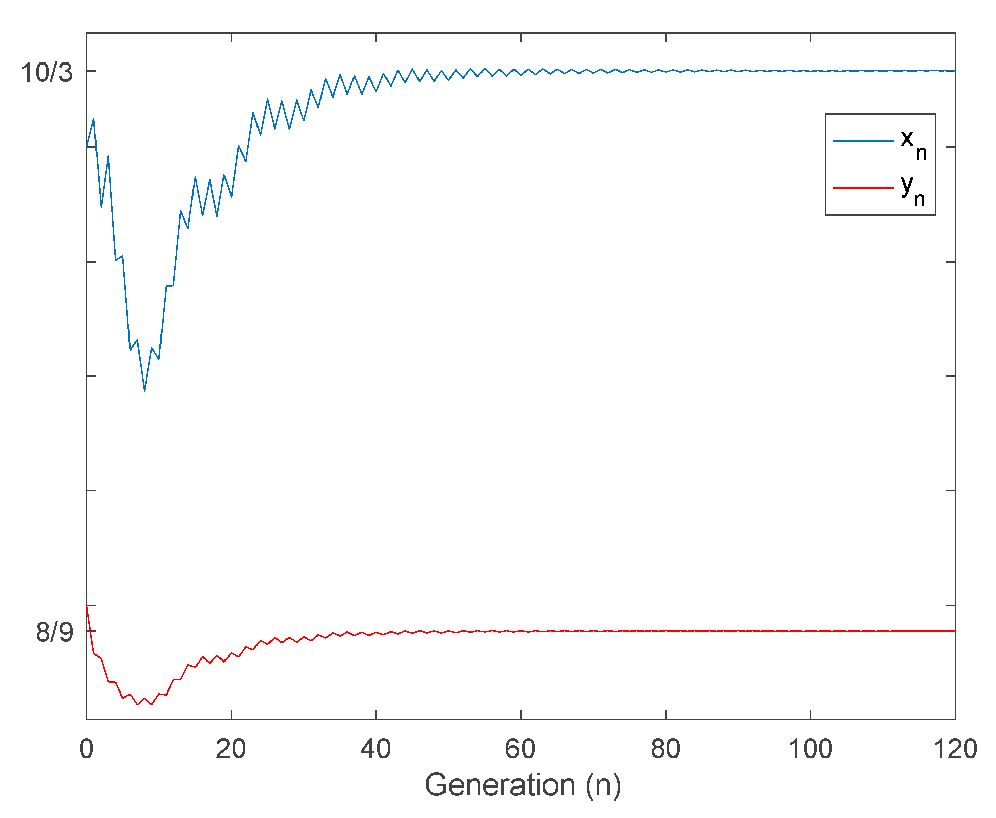
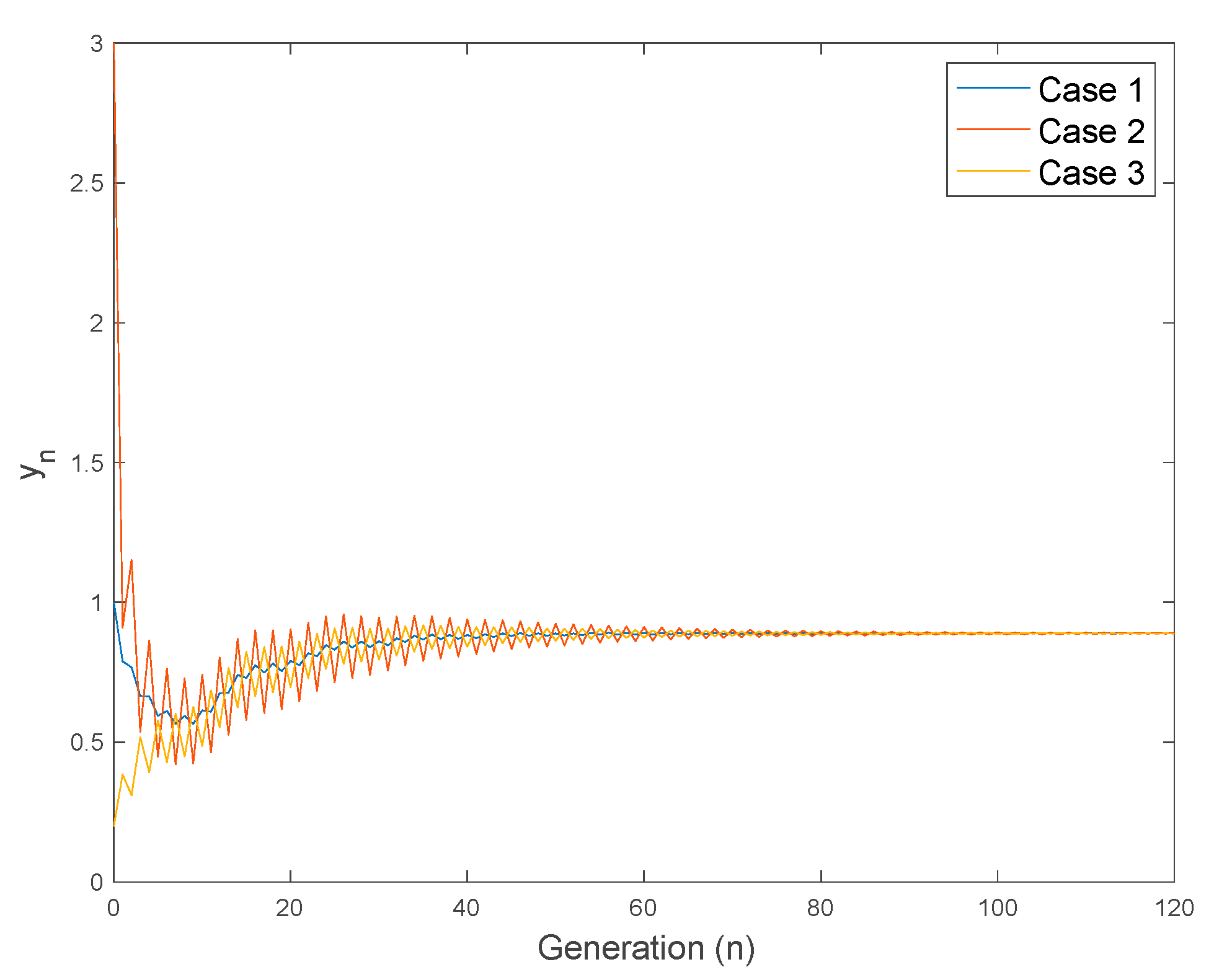
4.1. Non-Negativeness, Boundedness, and Location of Equilibrium Points

Consider the stage-structured model (1) parameterized by the following sequences:

$$\begin{array}{c}{\alpha }_n=5+sin(2\pi 0.1n), {\gamma }_n=0.4+0.1cos(2\pi 0.1n), \\ {\eta }_{1n}=0.15\left(1+e^{-0.1n}\right), {\eta }_{2n}=0.15\left(1+e^{-0.15n}\right)\end{array}$$

with positive initial conditions given by $x_0=0.2$ and $y_0=0.1$. These sequences are generation-dependent and their order of magnitude is similar to that considered in [1]. A periodic behavior has been selected for ${\alpha }_n$ and ${\gamma }_n$ in order to mathematically describe a seasonal behavior of the birth and maximum progression rates, which is typical in the reproduction cycles of many animals [27]. Thus, these values were selected as a periodic variation around a positive value in order to account for this biological fact. According to Proposition 5, the sequences ${\left\{x_n\right\}}_{n=0}^{\infty }$ and ${\left\{y_n\right\}}_{n=0}^{\infty }$ remain non-negative and bounded with an upper-bound given by $x_{n+1}\le \frac{{\alpha }_n{\gamma }_{n-1}}{{\eta }_{2,n-1}}$ and $y_{n+1}\le \frac{{\gamma }_n}{{\eta }_{2n}}$, respectively. This fact is illustrated in Figure 1 and Figure 2, where the evolution of ${\left\{x_n\right\}}_{n=0}^{\infty }$ and ${\left\{y_n\right\}}_{n=0}^{\infty }$ is displayed, respectively. In these figures it can be observed that the elements of both sequences are positive at all times while remaining bounded. In addition, the upper bounds for both sequences are also depicted in Figure 1 and Figure 2, showing that the actual value of the populations rest under their threshold. These figures support, thus, the results stated in Proposition 5. Moreover, from Figure 1 and Figure 2 it can also be deduced that the calculated upper bounds are somewhat conservative, in the sense that the actual values for the populations are far from the upper bound. Therefore, the calculation of a tighter upper bound appears to be a remaining open problem.

Furthermore, Proposition 7 discusses the location of the equilibrium points along with the conditions under which these exist. In order to numerically check the results claimed in Proposition 7, we consider the following parameterization for the model sequences:

$$\begin{array}{c}{\alpha }_n=5+e^{-0.1n}sin(2\pi 0.1n), {\gamma }_n=0.4+0.1e^{-0.3n}cos(2\pi 0.1n), {\eta }_{1n}=0.15\left(1+e^{-0.1n}\right), \\ {\eta }_{2n}=0.15\left(1+e^{-0.15n}\right). \end{array}$$

Now, all the sequences converge to the positive constant values:

$${\left\{{\alpha }_n\right\}}_{n=0}^{\infty }\to \alpha =5, {\left\{{\gamma }_n\right\}}_{n=0}^{\infty }\to \gamma =0.4, {\left\{{\eta }_{1n}\right\}}_{n=0}^{\infty }\to {\eta }_1=0.1, {\left\{{\eta }_{2n}\right\}}_{n=0}^{\infty }\to {\eta }_2=0.15.$$

Notice that under these values, the condition

$$1<\sqrt{\alpha \gamma }=1.4142<\frac{1}{2}\left(1-\frac{{\eta }_2}{{\eta }_1}\right)+\frac{\sqrt{{\left({\eta }_1+{\eta }_2\right)}^2+4{\eta }_1{\eta }_2\left(\alpha \gamma -1\right)}}{2{\eta }_1}=1.5$$

holds. Consequently, according to Proposition 7 there exists a positive equilibrium point with coordinates:

$$\begin{array}{c}{x}_{e1}=\frac{\sqrt{{\left({\eta }_1+{\eta }_2\right)}^2+4{\eta }_1{\eta }_2\left(\alpha \gamma -1\right)}-\left({\eta }_1+{\eta }_2\right)}{2{\eta }_1{\eta }_2}=\frac{10}{3}\\ y_e=\frac{\gamma x_e}{1+{\eta }_2{x}_e}=\frac{8}{9}\end{array}$$

which is locally asymptotically stable. The following Figure 3 depicts the evolution of both populations with the above considered parameterization.

The final values for both populations obtained from simulation are given by $x_{end}=3.3327$ and $y_{end}=0.889$, which are in great accordance with the theoretical values presented in Proposition 7 and calculated above. Furthermore, it can be observed that the populations are positive and remain bounded as stated in Proposition 5. Moreover, Figure 4 and Figure 5 show the evolution of both populations for different initial conditions given by: Case 1: $x_0=3$ and $y_0=1$; Case 2: $x_0=4$ and $y_0=3$; and Case 3: $x_0=1$ and $y_0=0.2$. As it is shown in Figure 4 and Figure 5, all the trajectories converge to the same equilibrium point, which is locally asymptotically stable, as it is claimed in Proposition 7(iii).

Finally, we now change the value of ${\left\{{\gamma }_n\right\}}_{n=0}^{\infty }$ to ${\gamma }_n=0.2+0.1e^{-0.3n}cos(2\pi 0.1n)$ so that the condition $\alpha \gamma =1$ holds. The initial conditions are $x_0=3$ and $y_0=1$. The Figure 6 displays the evolution of both populations in this case.

In Figure 6 it is shown that both populations converge to the extinction equilibrium point corresponding to $\left(x_e ,y_e\right)=\left(0 , 0\right)$. If we now complete a simulation for a large number of generations and make a zoom on the last part of it, we obtain Figure 7. In this Figure it is shown that the trajectories do not asymptotically converge to the extinction point, but they remain close to it since this point is not locally asymptotically stable as, concluded in Proposition 7(ii). Therefore, this Section illustrates some of the theoretical results contained in Section 2 regarding the non-negativity, boundedness, and existence of equilibrium points of the stage-structured model (1).

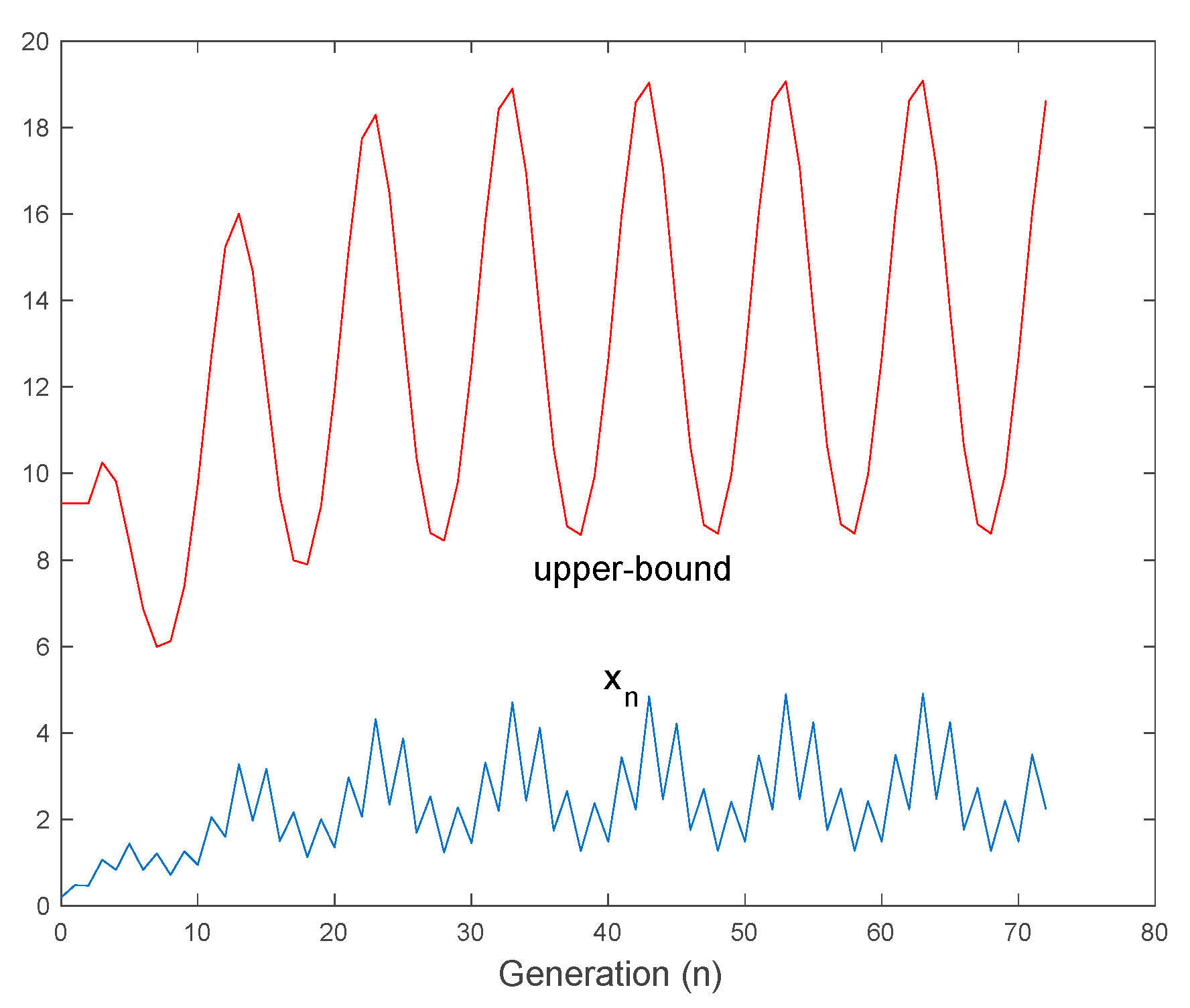
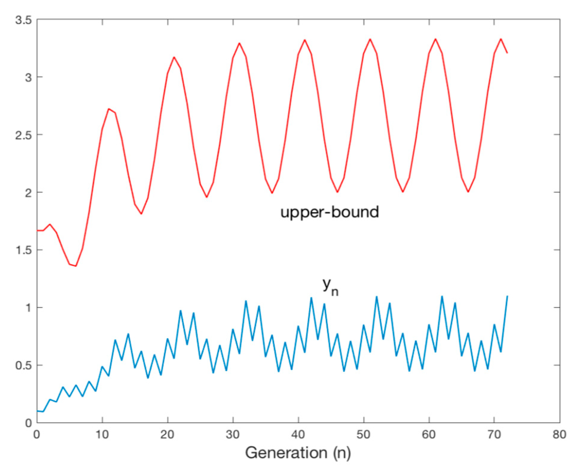
4.2. Oscillatory Solutions

In this Section, a numerical example concerning the oscillatory character of the solution of the stage-structured model (1) is presented. Thus, consider the sequences given by:

$$\begin{array}{c}{\alpha }_n=5+sin(2\pi 0.1n) {\gamma }_n=k_{2n}{g}_n=1.5+0.6cos(2\pi 0.1n), \\ {\eta }_{1n}=0.15\left(1+e^{-0.1n}\right), {\eta }_{2n}=0.15\left(1+e^{-0.15n}\right)\end{array}$$

with $k_{2n}=1$. The Figure 8 shows the shape of sequence ${\left\{{\gamma }_n\right\}}_{n=0}^{\infty }$.

From Figure 8 we can observe that there exist intervals where the sequence takes values smaller than unity, while on other intervals the values are larger than unity. Thus, it is easy to deduce that we can find two constants $k_1,k_2$ such that ${\displaystyle {\prod }_{i=n}^{n+k_1\left(n\right)}\left[{\gamma }_i\right]}\le 1$ and ${\displaystyle {\prod }_{i=n+k_1\left(n\right)+1}^{n+k_2\left(n\right)}\left[{\gamma }_i\right]}\ge 1$. Consequently, we are in the position to apply Proposition 9 and conclude that the solution to the stage-structured model (1) with this parameterization will be oscillatory. Figure 9 displays the solution of system (1), corroborating the result concluded from Proposition 9.

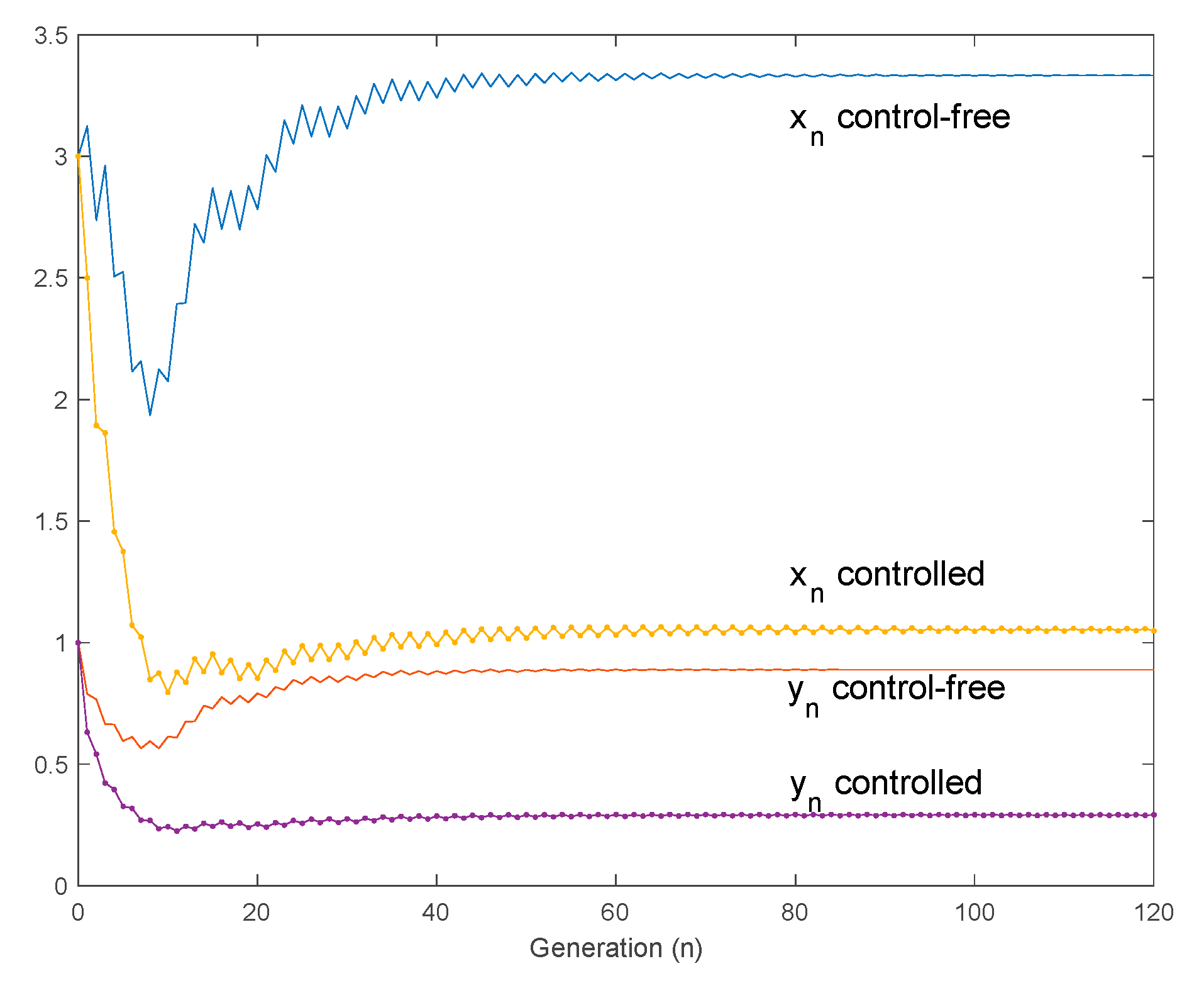
4.3. Use of Controls to Reduce the Larvae and Adult Mosquito Populations

In this last subsection, a simulation example concerning the use of controls to reduce the larvae and adult mosquito populations is considered. Thus, consider the sequences given by:

$$\begin{array}{c}{\alpha }_n^0=5+e^{-0.1n}sin(2\pi 0.1n), {\gamma }_n^0=0.4+0.1e^{-0.3n}cos(2\pi 0.1n), \\ {\eta }_{1n}=0.15\left(1+e^{-0.1n}\right), {\eta }_{2n}=0.15\left(1+e^{-0.15n}\right)\end{array}$$

where ${\alpha }_n^0$ and ${\gamma }_n^0$ are referred to as the nominal control-free values. The evolution of larvae and adult mosquito populations under this parameterization are displayed in Figure 3. As it is observed in Figure 3, both populations converge to finite positive values, which are the equilibrium points. The objective of using controls is to reduce the values of these populations. To this end we follow Example 4 guidelines. Thus, we take ${\alpha }_n\in {\left[{\alpha }_n^{\left(1\right)}, {\alpha }_n^{\left(2\right)}\right]}^{}$ and ${\gamma }_n\in {\left[{\gamma }_n^{\left(1\right)}, {\gamma }_n^{\left(2\right)}\right]}^{}$ with ${\alpha }_n^{\left(1\right)}=0.6{\alpha }_n^{\left(0\right)}$, ${\alpha }_n^{\left(2\right)}=0.9{\alpha }_n^{\left(0\right)}$, ${\gamma }_n^{\left(1\right)}=0.6{\gamma }_n^{\left(0\right)}$ and ${\gamma }_n^{\left(2\right)}=0.9{\gamma }_n^{\left(0\right)}$. In particular in this simulation example the constant values of ${\alpha }_n^{}=0.8{\alpha }_n^{\left(0\right)}$ and ${\gamma }_n^{}=0.8{\gamma }_n^{\left(0\right)}$ are employed. Figure 10 compares the control-free evolution of populations with the controlled case.

As it is observed in Figure 10, the control of the birth and maximum progression rate sequences allows for reducing the number of larvae and adult mosquitos, since the equilibrium point attained by the model is given by lower values than with the control-free situation. Furthermore, assume that the natural dynamics of the system for nominal parameters given by ${\alpha }_n^0\to {\alpha }_{}^0$ and ${\gamma }_n^0\to {\gamma }_{}^0$ make the system converge to the equilibrium point given by

$$x_e^0=\frac{\sqrt{{\left({\eta }_1+{\eta }_2\right)}^2+4{\eta }_1{\eta }_2\left({\alpha }^0{\gamma }^0-1\right)}-\left({\eta }_1+{\eta }_2\right)}{2{\eta }_1{\eta }_2} y_e^0=\frac{\gamma x_e^0}{1+{\eta }_2{x}_e^0}$$

so that the achieved values are not biologically acceptable. We would like to reduce them to the values $x_e^{}<x_e^0$ and $y_e^{}<y_e^0$. To this end, we would calculate the necessary values of the birth and progression rates $\alpha$, $\gamma$ from the above equations, so as to get the desired new equilibrium point $(x_e^{},y_e^{})$ as:

$$\begin{array}{c}\gamma =\frac{y_e^{}\left(1+{\eta }_2{x}_e^{}\right)}{x_e^{}}\\ \alpha =\frac{1}{\gamma }\left(\frac{{\left(2{\eta }_1{\eta }_2{x}_e^{}+\left({\eta }_1+{\eta }_2\right)\right)}^2-{\left({\eta }_1+{\eta }_2\right)}^2}{4{\eta }_1{\eta }_2}+1\right)=\frac{x_e^{}}{y_e^{}\left(1+{\eta }_2{x}_e^{}\right)}\left(\frac{{\left(2{\eta }_1{\eta }_2{x}_e^{}+\left({\eta }_1+{\eta }_2\right)\right)}^2-{\left({\eta }_1+{\eta }_2\right)}^2}{4{\eta }_1{\eta }_2}+1\right).\end{array}$$

The last step is to calculate the amount of insecticide that must be sprayed in the atmosphere to achieve these birth and progression rates. The relationship between the amount of insecticide and the attained values for the rates depends on the spraying method and other environmental characteristics. Once the amount of insecticide is calculated, the effect of overdose and its environmental impact can be specifically considered. In this way, the formulation developed in Section 3 allows for designing feasible values for these sequences. Overall, the presented numerical examples corroborate some of the theoretical results discussed in the previous Section 2 and Section 3.

5. Conclusions

In this paper, the mathematical formulation of a stage-structured model of larvae and adult mosquito populations has been presented. The model is described by time-varying parameters in order to account for their potentially seasonal dependence. This situation is accepted to be of practical importance due to the typical seasonal behavior of reproduction cycles in many animal populations. The work also investigated the conditions under which the model remains non-negative, possesses attainable equilibrium points, and is bounded and/or oscillatory. These conditions are derived in terms of the sequences parameterizing the system or in the terms of its asymptotic limits, when they exist. Consequently, the paper provides useful conditions to determine when equilibrium points exist and where they are located. The value of equilibrium points inform of the steady-state larvae and mosquito populations. When these values are not acceptable for environmental or human reasons, the paper proposes the way to change the birth and progression rates in order to perform control on them. This information is necessary to calculate the amount of insecticide that should be sprayed. It has also to be taken into account the seasonal temperature, the diet stocks for larvae, and the local density effects in order to accommodate the saturated values of the maximum progression rates to be used in the control feedback implementation. Worked illustrative examples have been developed. On the other hand, further numerical simulation examples corroborate the described theoretical results.

References

1. Li, Y.; Li, J. Stage-structured discrete-time models for interacting wild and sterile mosquitoes with Beverton- Holt survivability. Math. Biosci. Eng. 2019, 16, 572–602. [Google Scholar] [CrossRef] [PubMed]
2. Fister, K.R.; McCarthy, M.L.; Oppenheimer, S.F.; Collins, C. Optimal control of insects through sterile insect release and habitat modification. Math. Biosci. 2013, 244, 201–212. [Google Scholar]
3. Flores, J.C. A mathematical model for wild and sterile species in competition: Immigration. Physica A 2003, 328, 214–224. [Google Scholar] [CrossRef]
4. Li, Y.; Li, J. Discrete-time models for releases of sterile mosquitoes with Beverton-Holt type for survivability. Richerche Di Mat. 2018, 67, 141–162. [Google Scholar] [CrossRef]
5. Li, J. Malaria model with stage-structured mosquitoes. Math. Biosci. Eng. 2011, 8, 753–768. [Google Scholar] [CrossRef]
6. Stevic, S. A short proof of the Cushing-Henson conjecture. Discret. Dyn. Nat. Soc. 2006, 2006, 1–5. [Google Scholar] [CrossRef]
7. de la Sen, M.; Alonso-Quesada, S. Control issues for the Beverton-Holt equation in ecology by locally monitoring the environment carrying capacity: Non-adaptive and adaptive cases. Appl. Math. Comput. 2009, 215, 2616–2633. [Google Scholar] [CrossRef]
8. de la Sen, M.; Alonso-Quesada, S. Model-matching-based control of the Beverton-Holt equation in ecology. Discret. Dyn. Nat. Soc. 2008, 2008, 2616–2633. [Google Scholar] [CrossRef]
9. de la Sen, M.; Alonso-Quesada, S. A control theory point of view on Beverton-Holt equation in population dynamics and some of its generalizations. Appl. Math. Comput. 2008, 215, 464–481. [Google Scholar] [CrossRef]
10. Cushing, J.M.; Henson, S.M. A periodically forced Beverton-Holt equation. J. Differ. Equ. Appl. 2008, 8, 1119–1120. [Google Scholar] [CrossRef]
11. de la Sen, M. The environment carrying capacity is not independent of the intrinsic growth rate for subcritical spawning stock biomass in the Beverton-Holt equation. Ecol. Model. 2007, 204, 2171–2273. [Google Scholar] [CrossRef]
12. Hui, Y.; Lin, G.; Sun, Q. Oscillation threshold for a mosquito population suppression model with time delay. Math. Biosci. Eng. 2019, 16, 7362–7374. [Google Scholar] [CrossRef] [PubMed]
13. Takahasi, S.E.; Miura, Y.; Miura, T. On convergence of a recursive sequence xn+1 = f(xn−1, xn). Taiwan. J. Math. 2006, 10, 631–638. [Google Scholar] [CrossRef]
14. Stevic, S. On the recursive sequence xn+1 = xn−1/g(xn). Taiwan. J. Math. 2002, 6, 405–414. [Google Scholar]
15. Verma, R.; Sehgal, V.K.; Nitin, V. Computational stochastic modelling to handle the crisis occurred during community epidemic. Ann. Data. Sci. 2016, 3, 119–133. [Google Scholar] [CrossRef]
16. Iggidr, A.; Souza, M.O. State estimators for some epidemiological systems. Math. Biol. 2019, 78, 225–256. [Google Scholar] [CrossRef] [Green Version]
17. Yang, H.M.; Ribas-Freitas, A.R. Biological view of vaccination described by mathematical modellings: From rubella to dengue vaccines. Math. Biosci. Eng. 2018, 16, 3185–3214. [Google Scholar]
18. Koivu-Jolma, M.; Annila, A. Epidemic as a natural process. Math. Biosci. 2018, 299, 97–102. [Google Scholar] [CrossRef]
19. Meyers, L. Contact network epidemiology: Bond percolation applied to infectious disease prediction and control. Bull. Am. Math. Soc. 2007, 44, 63–86. [Google Scholar] [CrossRef] [Green Version]
20. de la Sen, M. On the design of hyperstable feedback controllers for a class of parameterized nonlinearities. Two application examples for controlling epidemic models. Int. J. Environ. Res. Public Health 2019, 16, 2689. [Google Scholar]
21. de la Sen, M. Parametrical non-complex tests to evaluate partial decentralized linear-output feedback control stabilization conditions for their centralized stabilization counterparts. Appl. Sci. 2019, 9, 1739. [Google Scholar] [CrossRef] [Green Version]
22. Cai, L.; Ai, S.; Li, J. Dynamics of mosquitoes populations with different strategies for releasing sterile mosquitoes. SIAM J. Appl. Math. 2014, 74, 1786–1809. [Google Scholar] [CrossRef]
23. Li, J.; Yuan, Z. Modelling releases of sterile mosquitoes with different strategies. J. Biol. Dyn. 2015, 9, 1–14. [Google Scholar] [CrossRef] [PubMed]
24. Pryce, J.; Choi, L.; Malone, D. Insecticide space spraying for preventing malaria transmission. Cochrane DB. Syst. Rev. 2017, 2017, CD012689. [Google Scholar] [CrossRef] [Green Version]
25. Smith, D.L.; Battle, K.E.; Hay, S.I.; Barker, C.M.; Scott, T.W.; McKenzie, F.E. Ross, McDonald and a theory for the dynamics and control of mosquito-transmitted pathogens. Plos Pathogens 2012, 8, e1002588. [Google Scholar] [CrossRef] [Green Version]
26. Couret, J.; Dotson, E.; Benedict, M.Q. Temperature, larval diet and density effects on development rate and survival of aedes aegypti (Dipta: Culicidae). PLoS ONE 2014, 9, e87468. [Google Scholar] [CrossRef]
27. Ackleh, A.S.; Jang, S.R.J. A discrete two-staged population model: Continuous versus seasonal reproduction. J. Differ. Equ. Appl. 2007, 13, 261–274. [Google Scholar] [CrossRef]
Figure 1. Evolution of the { x n } n = 0 population and its calculated upper bound.
Mathematics 07 01181 g001
Figure 2. Evolution of the { y n } n = 0 population and its calculated upper bound.
Mathematics 07 01181 g002
Figure 3. Evolution of { x n } n = 0 and { y n } n = 0 populations.
Mathematics 07 01181 g003
Figure 4. Evolution of { x n } n = 0 for different initial conditions.
Mathematics 07 01181 g004
Figure 5. Evolution of { y n } n = 0 for different initial conditions.
Mathematics 07 01181 g005
Figure 6. Evolution of { x n } n = 0 and { y n } n = 0 populations when α γ = 1 .
Mathematics 07 01181 g006
Figure 7. Zoom on { x n } n = 0 and { y n } n = 0 populations when α γ = 1 for a large number of generations.
Mathematics 07 01181 g007
Figure 8. Evolution of the sequence { γ n } n = 0 .
Mathematics 07 01181 g008
Figure 9. Oscillatory character of { x n } n = 0 and { y n } n = 0 populations.
Mathematics 07 01181 g009
Figure 10. Comparison between the control-free and the controlled evolution of larvae and adult mosquito populations.
Mathematics 07 01181 g010