3.1. Application of Family (3) to Fisher’s Equation
Fisher’s equation [
11]
represents a model of diffusion in population dynamics, where
is the diffusion constant,
r is the growth rate of the species, and
c is the carrying capacity. In this section, a specific case of Fisher’s equation is solved using iterative methods. In this case,
, so (
15) gets into
The domain of
x is the interval
. The boundary conditions are
and
, for
, while the initial condition is
Discretizing (
16) and by using divided differences, the problem can be solved as a family of nonlinear systems. For this purpose, we first have selected a grid of points in the domain,
, where
represents the node in the spatial variable, set as
,
j is the index of the time variable, set as
h and
k are the spatial and time steps, respectively, and
and
are the number of subintervals for variables
x and
t, respectively. Then, an approximation of the solution at each point
of the mesh will be obtained, that is,
.
Applying backward differences to the time derivative and central differences to the spacial one, that is
the scheme in finite differences for the approximated problem is
for
,
. After some algebraic manipulations, (
18) results in
where
. Depending on the number of subintervals used in the discretization of the variable
x, a nonlinear system of size
can be found by solving (
19). The nonlinear system defined for a fixed
j is the following:
where matrix
A is
Each system gives an approximated solution for the problem in a time step
from the obtained in the instant
, so we begin to solve the systems using the solution at
provided by (
17).
Using iterative methods for solving nonlinear systems, such as family (
3), system (
20) can be solved. In order to compare the numerical results, another iterative scheme with the same order of convergence as family (
3) has been chosen. In this case, the Sharma et al. [
12] method, denoted in this work by
, is fourth-order convergent and has the iterative expression
where
.
On the other hand, to check the numerical behavior of family (
3), it is necessary to select a weight function satisfying conditions of Theorem 2, so it will be obtained a method of this family. Several functions satisfy the conditions of the theorem, some of them being:
An efficiency comparison between the proposed schemes is given in terms of the computational cost and the number of functional evaluations. This comparison helps to choose the more efficient method of family (
3). For this purpose, we can use the efficiency index defined by Ostrowski [
13] as
, where
p is the order of the method and
d is the number of new functional evaluations per iteration required by the method. The computational cost for solving a linear system of equations depends on its size. As the proposed methods can be used for solving large systems of equations, this cost must be taken into account. Thus, we compare the performance of the methods with the computational efficiency index introduced in [
7] as
, where
is the number of operations (products and quotients) per iteration.
Table 1 summarizes the results for the computational efficiency index and number of functional evaluations for each method, where
,
, and
denote the resulting iterative schemes when family (
3) is applied using the weight functions (
22), respectively.
For each method,
Table 1 shows the number of different evaluations of the function (
F), the Jacobian matrix (
), and the number of different divided differences used by the method in each iteration (nDD). All the methods need
n and
evaluations to compute
F and
, respectively, and
for each divided difference operator.
Regarding the operational cost, the value of Mv is the number of matrix–vector products, with operations for each product. To compute an inverse linear operator, one may solve a linear system of equations, where an LU decomposition is performed and two triangular systems must be solved, with a total cost of operations. However, for solving r linear systems with the same matrix of coefficients, the LU decomposition is computed only once, so the computational cost is only . The values of s1 and s2 are the number of linear systems that each scheme solves per iteration with matrix of coefficients or another matrix, respectively.
As the results of
Table 1 show, among the methods belonging to family (
3), the most efficient is method
. Then, the numerical performance of the family is carried out with this method. In addition, method
requires more functional evaluations than the other ones as it computes two Jacobian matrices in each iteration.
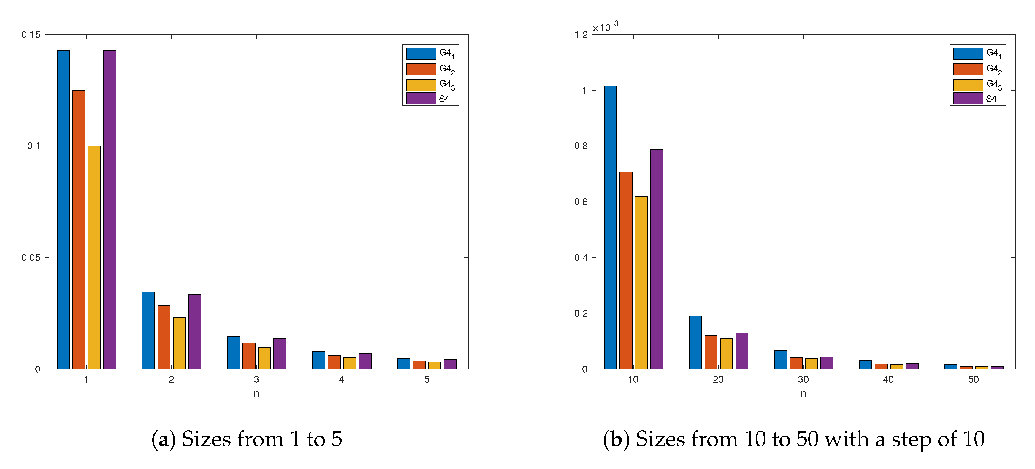
The results obtained in
Table 1 can be observed in
Figure 1, where the value of
for the four methods by varying the size of the system (
n) has been represented. As we can see, for small values of
n, the indices of
and
show similar performance; meanwhile, when the value of
n increases, the computational efficiency index of all methods decreases, but the index of method
is greater than the rest.
We have solved system (
20) using methods
and
for
. For the numerical performance, we use software Matlab R2017b with variable precision arithmetics of 1000 digits of mantissa.The results of the application of the methods for solving the nonlinear system are collected in
Table 2 varying the value of
and
. For every performance, the iteration procedure stops when
or the number of iterations reaches the number 50. The value of iter represents the mean number of iterations needed when all the columns have been calculated and the terms
represent the value
. Moreover, the elapsed time in seconds to obtain the solution for the problem after 10 (consecutive) executions is shown.
The results in
Table 2 show the good performance of method
for solving the Fisher’s problem. Method
only needs two iterations to calculate a solution for the system, the mean number of iterations always being lower than that of method
. For a fixed value of
, when
increases, so does the elapsed time, but the approximation to the solution is better since
is smaller. In addition, the e-time is lower for method
, so it reaches the solution with more computational efficiency and arithmetical precision than the other scheme.
3.2. Application of Family GH to Nonlinear Test Systems
According to the results obtained in
Table 1 for methods
, the numerical experiments for family (
13) are developed by using the following weight functions:
which satisfy conditions of Theorem 3.
To compare the features of our method with other schemes of the literature, the numerical tests are also performed on two iterative schemes of order 8 that can be found in [
5,
14]. The method is named
, for our iterative family using functions (
23),
for [
5], and
, for [
14]. The computational efficiency index and the number of functional evaluations of these methods are collected in
Table 3.
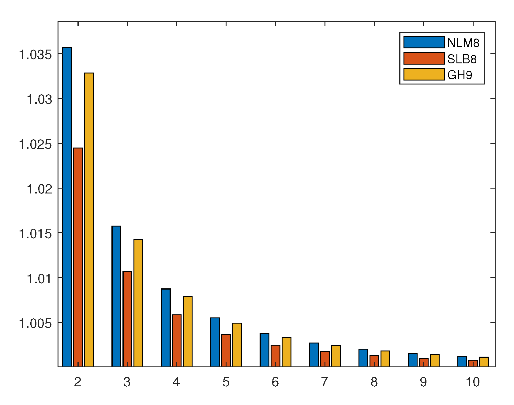
Method
requires few functional evaluations, as low operational cost and has a competitive computational efficiency index (see
Figure 2). We will see now that the numerical experiments confirm these results. For this purpose, methods
,
, and
are applied to solve the following nonlinear systems:
- (a)
, where
- (b)
, such that
- (c)
, where
The results obtained from applying the methods for solving the nonlinear systems are collected in
Table 4,
Table 5 and
Table 6. The stopping criteria now is a difference between two consecutive iterates lower than
or the condition
with a maximum number of iterations of 50. The results have been calculated using Matlab R2017b with variable precision arithmetics of 2000 digits of mantissa. In this way, the numerical noise is far enough to not affect the final result. The approximated computational order of convergence [
15] represents an approximation of the order of convergence of each method.
The ACOC [
15] is the approximated computational order of convergence defined as
It is a computational approximation of the theoretical order.
For every nonlinear system, the higher value of the ACOC is for the GH family, as expected. In general, our proposed scheme converges in less iterations than the other tested methods with very competitive error estimates.


