Article

Fractional Derivatives: The Perspective of System Theory

by
Manuel Duarte Ortigueira
1 and
José Tenreiro Machado
2,*
1
CTS–UNINOVA and DEE of NOVA, School of Science and Technology, Nova University of Lisbon, Campus da FCT da UNL, Quinta da Torre, 2829–516 Caparica, Portugal
2
Department of Electrical Engineering, Institute of Engineering, Polytechnic of Porto, R. Dr. António Bernardino de Almeida, 431, 4249–015 Porto, Portugal
*
Author to whom correspondence should be addressed.
Mathematics 2019, 7(2), 150; https://doi.org/10.3390/math7020150
Submission received: 31 December 2018 / Revised: 21 January 2019 / Accepted: 25 January 2019 / Published: 5 February 2019
(This article belongs to the Special Issue Fractional Integrals and Derivatives: “True” versus “False”)

Abstract

:
This paper addresses the present day problem of multiple proposals for operators under the umbrella of “fractional derivatives”. Several papers demonstrated that various of those “novel” definitions are incorrect. Here the classical system theory is applied to develop a unified framework to clarify this important topic in Fractional Calculus.

1. Introduction

The name fractional derivative (FD) is assigned to several mathematical operators, namely the Grünwald-Letnikov (GL), Liouville (L), Riemann-Liouville (RL), Caputo (C), Marchaud, Hadamard (H), Riesz, and others [1,2,3,4,5]. They are considered as generalisations of the classical derivative studied by Leibniz, Newton, Euler, and Lagrange, just to name a few of the most important mathematicians [1,2,6,7,8,9,10]. In previous papers we contributed to the on-going debate about the pros and cons of each formulation and we proposed possible approaches coherent with classic results in Science and Engineering [11,12]. In recent years, several operators were suggested claiming to be a “fractional derivative”. This state of affairs motivated several papers showing the incorrectness of using the designation FD and even, in several cases, the absence of novelty [13,14,15,16,17]. We proposed a coherent framework for deciding if a given operator is a FD by formulating two criteria [11]. Nevertheless, the debate and the controversy remain. Some questions require suitable answers:
  • What do we mean by “derivative”?
  • What is the relation between derivative and integral?
  • Frequently different notions of “integral” are mixed. Should not we use different notations or distinct names?
  • When can we say that an operator is fractional?
  • Should we consider a framework where integer and non integer orders co-exist and are mixed?
  • What do we mean by fractional calculus? Should it be the calculus involving, at least, one “non integer order” derivative?
  • Can we consider as “fractional operator” any expression involving a convolution of a function and a given kernel?
  • Is it reasonable to choose a classic operator, to change its form by introducing a parameter and to call it FD?
  • How can we call “fractional derivative” to an operator that is itself solution of a linear differential equation?
  • The existence of a non integer parameter is reason for the use of the word “fractional”?
Several of these questions and others were discussed in round tables in the scope of several meetings held by the fractional calculus community [18,19]. Nevertheless, present day state of affairs reveals that they were not sufficient to stimulate all researchers for a systematic definition of the fundamental concepts. We observe the emergence of a plethora of assumed new operators that are named as novel or generalised fractional derivatives. Often it is also claimed that such operators fit better the experimental data. Obviously, from an application point of view, such lightly written words would need a systematic and solid testing with data from many distinct scientific areas, and the comparison with the results provided by classical derivatives (it is important to remark that this requires long observation intervals to capture long range memory effects). Furthermore, from a formal point of view, the good or bad fit into data, or the so-called “generalisation” by modifying some kernel, are not necessarily correct in mathematical terms when thinking on the properties of FD. Quoting Henri Poincaré Mathematics has a threefold purpose. It must provide an instrument for the study of nature. But this is not all: it has a philosophical purpose, and, I dare say, an aesthetic purpose. The main aim in this paper is to continue the discussion and try to establish a framework for avoiding misinterpretations and controversial or, even the incorrect, use of definitions.
Having these ideas in mind, this paper is organized as follows. Section 2 introduces the main terms and assumptions adopted in the follow-up. Section 3 recalls the definitions and fundamental properties of classic derivatives. Several aspects for the unification of concepts in the perspective of system theory are also discussed. Motivated by these ideas, Section 4 addresses the definition of fractional derivative. In these initial sections we assume that the independent variable t is continuous. However, computational systems are being increasingly important. Section 5 considers the case of the “discrete-time” operators. Finally, in Section 6 several conclusions and additional comments are presented.

2. Glossary and Assumptions

In Science it is important to define precisely the concepts that we are talking about. In fractional calculus there is a considerable confusion in the adopted terminology having, in some cases, different names for the same operator. Here we try to clarify the meaning for different terms in order to avoid such problem. Therefore, we start with some fundamental terms. Later, when necessary, we will introduce others, that are necessary in the rest of the paper.
  • Anti-causal
    An anti-causal system is causal under reverse time flow. A system is anti-causal if the output at any instant depends only on values of the input at the present and future time.
  • Anti-derivative
    The operator that is simultaneously the left and right inverse of the derivative will be called anti-derivative. It will be used to compute the definite integral through the Barrow formula [20]. This should be not confused with the negative order derivative, that needs not to be inverse of a derivative.
  • Backward
    Reverse time flow—from future to past.
  • Causal operator or system
    A system is causal if the output at any instant depends only on values of the input at the present and past time [21].
  • Derivative
    Derivative (first order) of a function, f ( t ) is the limit of the ratio of the change in such function to the corresponding change in its independent variable as the latter change approaches zero. It will be represented by D f ( t ) , f ( t ) , or d f ( t ) d t .
  • Forward
    Normal time flow—from past to future.
  • Fractional
    Fractional will have the meaning of non integer real number.
  • Integral
    In strict mathematical therms, there are several definitions of integral. However, the simplest is the Riemann integral that we can state as the numerical measure of the area under the graph of a given positive function, above the horizontal axis, and bounded on the sides by ordinates drawn at the endpoints of a specified interval. This is usually called definite integral and it is distinct from the indefinite integral, also called primitive.
  • Primitive
    The operator that is only the right inverse of the derivative will be called primitive.
This paper tries to answer some of the initial questions. To clarify concepts, we adopt the designation “unified derivative” instead of “fractional derivative”.
We assume that
  • We work on R . Nonetheless, this is not a limitation. If the function at hand is defined on any sub-interval in R , we can extend the definition of the function to the whole real line with null values.
  • We do not address the proof of existence of the operators.
  • We use the two-sided Laplace transform (LT):
    F ( s ) = L f ( t ) = R f ( t ) e s t d t ,
    where f ( t ) is any function defined on R and F ( s ) is its transform, provided that it has a non empty region of convergence
  • The Fourier transform (FT), F f ( t ) , is obtained from the LT through the substitution s = i ω with ω R and i = 1
  • The functions and distributions have Laplace and/or Fourier transforms
  • Current properties of the Dirac delta distribution, δ ( · ) , and its derivatives, δ ( · ) , δ ( · ) , will be used
  • The standard convolution operation will be adopted
    f ( t ) g ( t ) = R f ( τ ) g ( t τ ) d τ .
  • The order of any fractional derivative, α , is any real number. We will not consider the complex order, since it gives non Hermitian derivatives.
  • The multi-valued expressions s α and ( s ) α will be used. To obtain functions from them we will fix for branch-cut lines the negative real half axis for the first and the positive real half axis for the second; for both the first Riemann surface is chosen.
  • The Heaviside unit step will be represented by ε ( t ) and the signum function by s g n ( t ) . These functions are related by s g n ( t ) = 2 ε ( t ) 1 .
  • We define the “floor” of a real number α as the integer N = α verifying N α < N + 1 .

3. The Classic Derivatives and Their Inverses

3.1. Elemental Derivatives

We find in the literature three standard definitions of (order 1) derivative [12] (the called quantum derivative will not be considered here [22]). These elemental derivatives can be considered as “seeds” for the notion of high level derivatives. Such derivatives are:
Definition 1.
  • Forward or causal
    D f f ( t ) = lim h 0 f ( t ) f ( t h ) h ,
  • Backward or anti-causal
    D b f ( t ) = lim h 0 f ( t + h ) f ( t ) h .
Remark 1.
Substituting h for + h interchanges the definitions, meaning that we only have to consider h > 0 .
• Two-sided or centred
D c f ( t ) = lim h 0 f ( t + h / 2 ) f ( t h / 2 ) h .
Remark 2.
The expression (5) was used in [23,24] to obtain two different two-sided (centred) fractional derivatives. Later, in Section 3.4, we will recover the general formulation of these derivatives.
Remark 3.
Most literature on Differential Calculus uses definition (4) only due to historical reasons.
In terms of the Laplace transform we have
  • Forward or causal
    L D f f ( t ) = lim h 0 1 e s h h F ( s ) = s F ( s ) ,
  • Backward or anti-causal
    L D b f ( t ) = lim h 0 e s h 1 h = s F ( s ) ,
  • Two-sided or acausal
    F D c f ( t ) = lim h 0 e s h / 2 e s h / 2 h F ( i ω ) = s F ( s )
Remark 4.
Note that, although different, the LT of the three derivatives is the same and valid in the whole complex plane.
It is straightforward to invert the relations (3) and (4), and we obtain
D f 1 f ( t ) = lim h 0 n = 0 f ( t n h ) · h ,
D b 1 f ( t ) = lim h 0 n = 0 f ( t + n h ) · h .
Using the LT, we have
L D f 1 f ( t ) = lim h 0 h n = 0 e s h F ( s ) = 1 s F ( s ) , R e ( s ) > 0 ,
L D b 1 f ( t ) = lim h 0 h n = 0 e s h F ( s ) = 1 s F ( s ) , R e ( s ) < 0 .
Remark 5.
Note the appearance of the regions of convergence (ROC) subsets of C . This important fact is tied with causality [21,25].

3.2. First Unification

The repeated use of the above derivatives and anti-derivatives leads to closed formulae valid for any integer order, N Z [12], such that:
D f N f ( t ) = lim h 0 + n = 0 ( N ) n n ! f ( t n h ) h N ,
D b N f ( t ) = ( 1 ) N lim h 0 + n = 0 ( N ) n n ! f ( t + n h ) h N ,
respectively, where ( a ) k = a ( a + 1 ) ( a + 2 ) ( a + k 1 ) denotes the Pochammer symbol. Expressions (13) and (14) reflect, in a unified way, all integer order derivatives and anti-derivatives. Therefore, we can use only the word derivative independently of having positive or negative order.
The corresponding LT are given by:
L D f N f ( t ) = s N F ( s ) , R e ( s ) > 0 ,
L D b N f ( t ) = s N F ( s ) , R e ( s ) < 0 ,
respectively. From the point of view of system theory, expressions (15) and (16) tell us that the derivative operator represents a system with transfer function (TF) given by H ( s ) = s N . In this perspective, we consider the system approach with the integer order derivatives formulated by means of the two-sided LT property L f ( n ) ( t ) = s n L f ( t ) , where n Z , and it becomes clear the meaning of the sequence
s n s 2 s 1 1 s 1 s 2 s n
in the Laplace domain. Indeed, the corresponding time sequence is
± t n 1 ( n 1 ) ! u ( ± t ) ± t 2 2 ! u ( ± t ) ± t 1 1 ! u ( ± t ) ± u ( ± t ) δ ( t ) δ ( t ) δ ( t ) δ ( n ) ( t )
that allows us to write, for the causal definition (the other case is similar),
D f N f ( t ) = 0 f ( t τ ) τ N 1 ( N 1 ) ! d τ ,
where we assume that, if N 0 , then τ N 1 ( N 1 ) ! = δ ( N ) ( τ ) .

3.3. Second Unification

It is straightforward to extend formulae (13) and (14) to any real order. In fact, with α R we can write
D f α f ( t ) = lim h 0 + n = 0 ( α ) n n ! f ( t n h ) h α ,
D b α f ( t ) = e i α π lim h 0 + n = 0 ( α ) n n ! f ( t + n h ) h α ,
that have LT
L D f α f ( t ) = s α F ( s ) , R e ( s ) > 0 ,
L D b α f ( t ) = s α F ( s ) , R e ( s ) < 0 ,
respectively. These relations, allow us to fill in the gaps in middle the discrete sequence (17) to obtain, for example
s n s π s 2 s 3 / 2 s 1 s 1 / 3 1 s 1 s 3 / 2 s 2 s n .
giving a meaning for s α , ± R e ( s ) > 0 . The inverse LT of this transfer function is
L s α = ± t α 1 Γ ( α ) ε ( ± t )
that leads to
D f α f ( t ) = 0 f ( t τ ) τ α 1 Γ ( α ) d τ ,
generalising the causal expression (19) to real orders. For the anti-causal case, we get the general expression:
D b α f ( t ) = e i α π 0 f ( t + τ ) τ α 1 Γ ( α ) d τ .

3.4. Third Unification

The factor e i α π in (27) was already included by Liouville [26] to guarantee that L D b α f ( t ) = s α F ( s ) , for R e ( s ) < 0 . It apeared also in the backward GL derivative (21) and particular integer order cases. However, this factor may be of no relevance in many applications, especially when the independent variable is space, not time. If this term is removed, then we can join pairs of formulae into only one. We change also the nomenclature, using left for forward and right for backward. Therefore, (20) and (21) lead to
D l , r α f ( t ) = lim h 0 + n = 0 ( α ) n n ! f ( t ± n h ) h α ,
where the signs − and + are used for the left and right derivatives, respectively. The corresponding Liouville integral formulations are expressed by
D l , r α f ( t ) = 0 f ( t ± τ ) τ α 1 Γ ( α ) d τ .
The LT of these derivatives are
L D l , r α f ( t ) = ( ± s ) α F ( s ) , R e ( ± s ) > 0 .
From these results we conclude that
  • We can combine two derivatives of any orders, α and β , to obtain a third derivative
    s α s β = s α + β
  • If f ( t ) = e i ω t , ω R , then
    D α e i ω t = ( ± ω ) α e i ω t = ω α e ± i α π 2 s g n ( ω ) e i ω t
    where the + and − signs refer to the left and right cases in (28) and (29), respectively.
  • The corresponding frequency responses are given by
    H ( i ω ) = ω α e ± i α π 2 s g n ( ω )
    This result is important, since it expresses very clearly the unification of the derivatives and motivates a further development as discussed in the next subsection.

3.5. Fourth Unification
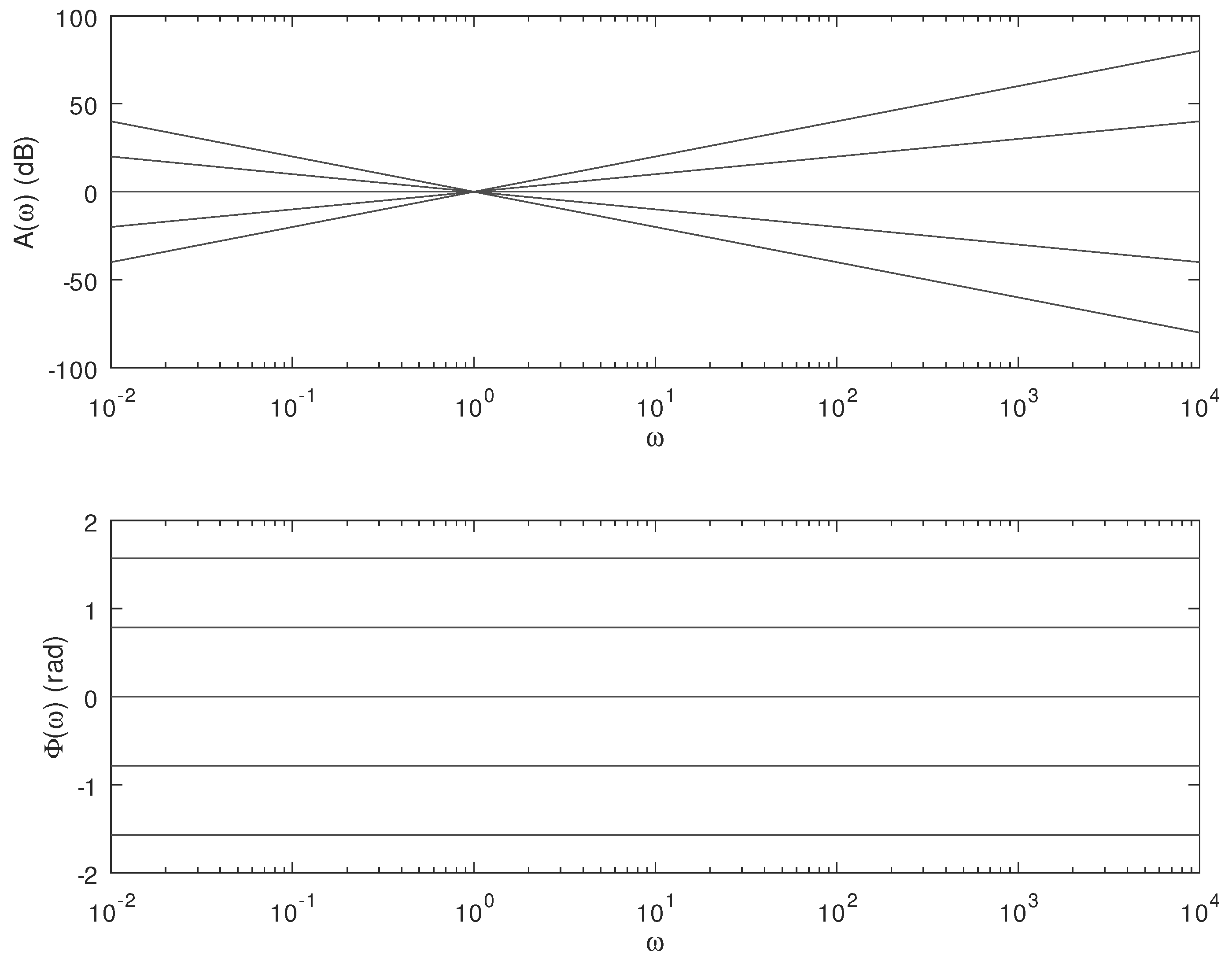
In (31) it is written that the combination of two derivatives of the same type (e.g., left) gives rise to another derivative of the same type. Now, we consider the combination of one derivative of each type.
Definition 2.
Consider two derivatives, causal and anti-causal, with orders α and β, having frequency responses ω α e i α π 2 s g n ( ω ) and ω β e i β π 2 s g n ( ω ) , respectively.
We define a new derivative with frequency response
Ψ θ γ ( i ω ) = ω γ e i θ π 2 s g n ( ω ) ,
where γ = α + β is the order of the derivative and θ = α β is the parameter of asymmetry (sometimes called skewness).
It can be shown [23,24] that, if γ > 1 , then the frequency response (34) corresponds to a two-sided derivative given by:
D c γ f ( t ) : = lim h 0 + h γ n = + ( 1 ) n · Γ γ + 1 Γ γ + θ 2 n + 1 Γ γ θ 2 + n + 1 f ( t n h ) .
Suitable choices of the parameters γ and θ allow us to recover the causal and anti-causal derivatives. The particular cases of α = β and α β = ± 1 are interesting and correspond to well-known operators as we will see later at Section 4.3.

3.6. Bode Diagrams

Bode diagrams are useful tools for the analysis and design of linear systems [21,25], since they provide a direct insight into models adopted in engineering and natural systems. This tool is of relevance when applied to the unified derivatives above discussed in Section 3.2, Section 3.3, Section 3.4 and Section 3.5.
Definition 3.
From formula (34) define two spectra (Figure 1):
  • Amplitude spectrum
    A ( ω ) = ω γ
  • Phase spectrum
    Φ ( ω ) = θ π 2 s g n ( ω )
For real-valued functions, the amplitude and the phase are even and odd functions, respectively [21,25]. For this reason, we only need to represent log plots for positive frequencies that are called Bode diagrams. For A ω it is usual to express the amplitude in deciBell (dB). Then, it results
A ( ω ) d B = γ 20 log ω
that is represented by a straight line with slop 20 γ dB per decade (dB/dec). The phase Φ ω is expressed in radians or degrees and represented by horizontal straight lines at α π 2 .
In Table 1, we consider some particular cases for the parameters γ and θ and we point out the name of the of resulting derivatives, assuming that α > 0 . We include also the Riesz and Feller potentials [1,2] that we will discuss in Section 4.
This list includes the most relevant examples of application of our framework. Some operators such as, for example, the Erdélyi and Kober integrals fall outside this point of view and should not be considered derivatives.
Remark 6.
It can be shown that the derivatives defined by means of (34) verify the usual properties required for the FD to follow, namely the strict sense criterion proposed in [11].

4. Derivative Definition Through Integral Formulations

4.1. Definition

The results from the previous section motivate the following definition of the unified derivative.
Definition 4.
We define the α-order “unified derivative” as the convolutional operator
D θ α f ( t ) = R f ( t τ ) ψ θ α ( τ ) d τ ,
where ψ θ α ( t ) , t R , is the kernel of the derivative and θ R , is an asymmetry parameter that controls the characteristics of the derivative, namely the causality. The kernel ψ θ α ( t ) is a function with Fourier transform Ψ θ α ( i ω ) , ω R , such that the corresponding Bode diagram of amplitude is a straight line with slope 20 α dB/dec and the phase is a horizontal straight line with value α π 2 .

4.2. A General Kernel

In (34) we obtained the frequency response of the unified derivative. If the inverse Fourier transform is ψ θ α ( t ) = F 1 ω α e i π 2 θ · s g n ( ω ) , then it is known [23,24] that:
ψ θ α ( t ) = sin α + θ · s g n ( t ) π 2 2 sin α π Γ ( α ) | t | α 1 .
This is the general kernel that allows us to express the integral formulation of the unified derivative that can be written as:
D θ α f ( t ) = 1 2 sin α π Γ ( α ) R f ( t τ ) sin α + θ · s g n ( τ ) π 2 | τ | α 1 d τ .

4.3. Some Particular Kernels

As seen above, the most interesting derivatives result from particular values of the parameters α and θ . Here, we analyse several cases as follows.
  • α = θ = N N 0
    In this case, Ψ θ γ ( i ω ) = i ω α and ψ N N ( t ) = δ ( N ) ( t ) . It yields
    D l N ( t ) = 0 f ( t τ ) δ ( N ) ( τ ) d τ = f ( τ ) δ ( N ) ( t τ ) d τ
    stating a well known property of the impulse distribution.
  • α = θ R +
    In this case, Ψ α α ( i ω ) = i ω α and ψ α α ( t ) = t α 1 Γ ( α ) ε ( t ) . We obtain
    D l α f ( t ) = 1 Γ ( α ) 0 f ( t τ ) τ α 1 d τ = 1 Γ ( α ) t f ( τ ) ( t τ ) α 1 d τ
    corresponding to the causal Liouville anti-derivative (line 2 in Table 1).
  • α R + and θ = α
    In this case, Ψ α α ( i ω ) = i ω α and ψ α α ( t ) = ( t ) α 1 Γ ( α ) ε ( t ) . Then, it results
    D r α f ( t ) = 1 Γ ( α ) 0 f ( t + τ ) τ α 1 d τ = 1 Γ ( α ) t f ( τ ) ( τ t ) α 1 d τ ,
    that corresponds to line 6 in Table 1.
  • α R + , θ = α
    Let Ψ α α ( i ω ) = i ω α . This is essentially the previous case 2 that leads to (43). However, the inverse FT produces a kernel that originates a singular integral. To avoid this problem we can use the properties of the pseudo-functions [27] that allow us to regularize (43) and use it for the derivative case. Let N = α + 1 . We can write (43) as [28]
    D l α f ( t ) = 1 Γ ( α ) 0 τ α 1 f ( t τ ) 0 N 1 ( ) m f ( m ) ( t ) m ! τ m d τ ,
    that we will call regularized Liouville derivative. Similar regularised integrals can be obtained for (44).
    Remark 7.
    If 0 < α < 1 and N = 1 , then we get
    D l α f ( t ) = 1 Γ ( α ) 0 τ α 1 f ( t τ ) f ( t ) d τ ,
    that coincides with the Marchaud derivative [1]. Nonetheless, for α > 1 , the Marchaud operator is no longer a derivative.
  • α R + , θ = α and N = α + 1
    In this case, we have two possibilities:
    (a)
    Ψ α α ( i ω ) = Ψ N N ( i ω ) Ψ α N α N ( i ω ) = i ω N i ω α N . This frequency response corresponds to a two-step derivative: integer order, N, derivative after a fractional anti-derivative of order N α . Instead of (41), we can write
    D l α f ( t ) = d N d t N 1 Γ ( α + N ) t ( t τ ) N α 1 f ( τ ) d τ ,
    that is called Liouville derivative [1] (line 3 in Table 1).
    (b)
    Ψ α α ( i ω ) = Ψ α N α N ( i ω ) Ψ N N ( i ω ) = i ω α N i ω N . It is the reverse of the above: a fractional anti-derivative of order N α after an integer order N derivative. Then, (41) assumes the form
    D l α f ( t ) = 1 Γ ( α + N ) t ( t τ ) N α 1 d N f ( τ ) d τ N d τ .
    that is called Liouville-Caputo derivative [10] (line 4 in Table 1).
    The corresponding right derivatives are easily obtained.
  • α R + , θ = 0
    In this case, Ψ 0 α ( i ω ) = ω α and the inverse FT of (40) is
    ψ 0 α ( t ) = 1 cos α π 2 Γ ( α ) | t | α 1 ,
    that leads to the Riesz potential (line 10 in Table 1)
    D 0 α f ( t ) = 1 cos α π 2 Γ ( α ) R f ( t τ ) | τ | α 1 d τ
  • α R + and θ = 1
    In this case, Ψ 0 α ( i ω ) = ω α and the inverse FT of (40) is
    ψ 0 α ( t ) = 1 sin α π 2 Γ ( α ) | t | α 1 s g n ( t ) .
    that leads to the Riesz-Feller potential (line 12 in Table 1)
    D 0 α f ( t ) = 1 sin α π 2 Γ ( α ) R f ( t τ ) | τ | α 1 s g n ( τ ) d τ
  • α = 0 and θ = 1
    In this case, Ψ θ 0 ( i ω ) = e i π 2 θ s g n ( ω ) = i s g n ( ω ) , and (40) leads to
    D 1 0 f ( t ) = 1 π f ( t τ ) 1 τ d τ
    which is the Hilbert transform of f ( t ) [21,25].
Remark 8.
We note that the scheme we presented is a theretical base for supporting the development and aplications of the FD. Practical problems may require some kind of modification—see for example [29].

4.4. Classic Riemann-Liouville, Caputo, and Hadamard derivatives

The classic formulations of Riemann-Liouville (RL) and Caputo (C) left derivatives ( α > 0 ) are obtained from the (47) and (48) assuming that f ( t ) is defined on a given interval a , b (we can set b = ). Therefore, for t a , b the RL and C derivatives are given by
R L D l α f ( t ) = D l N 1 Γ ( α + N ) a t ( t τ ) N α 1 f ( τ ) d τ
C D l α f ( t ) = 1 Γ ( α + N ) a t ( t τ ) N α 1 f ( N ) ( τ ) d τ ,
respectively, where N = α + 1 .
Remark 9.
It is important to note that, although the function f ( t ) has bounded support, both derivatives define non bonded support functions.
Concerning the Hadamard derivative and anti-derivative cases and for α > 0 , we have [2]
H D α [ f ( x ) ] = x d d x N 1 Γ ( N α ) a x log x ξ N α + 1 f ( ξ ) d ξ ξ
and
H D α [ f ( x ) ] = 1 Γ ( α ) a x log x ξ α 1 f ( ξ ) d ξ ξ .
With the change of variable inside the integral, that is, with ξ = e τ and x = e t , we obtain a derivative of the RL type.

5. On the Discrete-Time Derivatives

There are several approaches into the discrete-time FD. The most interesting are
  • The methodology based on time scales [30,31,32] that uses the nabla and delta derivatives;
  • Infinite series based on the approaches by Tarasov [33,34].
The first approach has more similarities with the theory we presented here and consists of the framework presented in [32]. In fact, the discrete-time derivatives described there recover the GL forward and backward derivatives introduced in (20) and (21). However, it is not straightforward to introduce some tool similar to Bode diagrams because:
  • The frequency response H ( i ω ) is obtained from the TF given by H ( s ) , when s assumes values on the Hilger circle: | s 1 h | = 1 h , where h is the sampling interval. Therefore, the domain is defined by ω π h , π h ;
  • The eigenvalue of the nabla derivative corresponding to the eigenvector e i ω h n is s = 1 e i ω h h . If h is very small, then s i ω . Therefore, only for small values of h the derivative is represented by straight lines in log plots;
  • There are no studies for the two-sided derivatives recovering to the one described in Section 3.5. The one proposed in [34] has a different formulation and properties.
From these considerations we conclude that the topic of discrete-time derivatives, requires still further study for keeping the simplicity of Bode diagrams.

6. Conclusions

This paper discussed the problem of multiple attempts to have distinct operators under the umbrella of “fractional derivatives”. One possible strategy is to discuss the validity of several operators recently proposed. Indeed, in previous papers it was demonstrated that such “novel” fractional derivatives are incorrect. Here we adopted an alternative strategy based on the classical system theory well known in applied sciences. Based on the tools of this theory we discussed a unified framework demystifying misleading, and often incorrect, formulations. Quoting again Henri Poincaré: To doubt everything, or, to believe everything, are two equally convenient solutions; both dispense with the necessity of reflection.

Author Contributions

These two authors contributed equally to this paper.

Funding

This work was funded by Portuguese National Funds through the FCT—Foundation for Science and Technology under the project PEst- UID/EEA/00066/2013.

Conflicts of Interest

The authors declare no conflict of interest.

Abbreviations

The following abbreviations are used in this manuscript:
FDFractional derivative
FIFractional integral
RLRiemann-Liouville
LLiouville
CCaputo
GLGrünwald-Letnikov
HHadamard

References

  1. Samko, S.; Kilbas, A.; Marichev, O. Fractional Integrals and Derivatives: Theory and Applications; Gordon and Breach Science Publishers: Amsterdam, The Netherlands, 1993. [Google Scholar]
  2. Kilbas, A.; Srivastava, H.; Trujillo, J. Theory and Applications of Fractional Differential Equations; North-Holland Mathematics Studies; Elsevier: Amsterdam, The Netherlands, 2006; Volume 204. [Google Scholar]
  3. Dugowson, S. Les Différentielles Métaphysiques. Ph.D. Thesis, Université Paris Nord, Villetaneuse, France, 1994. [Google Scholar]
  4. Kiryakova, V. A long standing conjecture failed? In Transform Methods and Special Functions; Institute of Mathematics and Informatics, Bulgarian Academy of Sciences: Sofia, Bulgaria, 1998; pp. 579–588. [Google Scholar]
  5. Kiryakova, V. A brief story about the operators of the generalized Fractional Calculus. Fract. Calc. Appl. Anal. 2008, 11, 203–220. [Google Scholar]
  6. Magin, R. Fractional Calculus in Bioengineering; Begell House Inc.: Redding, CT, USA, 2006. [Google Scholar]
  7. Tarasov, V.E. Fractional Dynamics: Applications of Fractional Calculus to Dynamics of Particles, Fields and Media; Nonlinear Physical Science; Springer: Beijing, China, 2010. [Google Scholar]
  8. Uchaikin, V.V. Fractional Derivatives for Physicists and Engineers: Background and Theory; Nonlinear Physical Science; Springer: Beijing, China, 2013. [Google Scholar]
  9. Ortigueira, M.D. Fractional Calculus for Scientists and Engineers, 2nd ed.; Lecture Notes in Electrical Engineering; Springer: Berlin/Heidelberg, Germany, 2011. [Google Scholar]
  10. Herrmann, R. Fractional Calculus: An Introduction for Physicists; World Scientific Publishing Co.: Singapore, 2011. [Google Scholar]
  11. Ortigueira, M.D.; Machado, J.A.T. What is a fractional derivative? J. Comput. Phys. 2015, 293, 4–13. [Google Scholar] [CrossRef]
  12. Ortigueira, M.; Machado, J.T. Which Derivative? Fract. Fract. 2017, 1, 3. [Google Scholar] [CrossRef]
  13. Tarasov, V.E. No violation of the Leibniz rule. No fractional derivative. Commun. Nonlinear Sci. Numer. Simul. 2013, 18, 2945–2948. [Google Scholar] [CrossRef]
  14. Ortigueira, M.D.; Machado, J.T. A critical analysis of the Caputo–Fabrizio operator. Commun. Nonlinear Sci. Numer. Simul. 2018, 59, 608–611. [Google Scholar] [CrossRef]
  15. Giusti, A. A comment on some new definitions of fractional derivative. Nonlinear Dyn. 2018, 93, 1757–1763. [Google Scholar] [CrossRef]
  16. Tarasov, V.E. No nonlocality: No fractional derivative. Commun. Nonlinear Sci. Numer. Simul. 2018, 62, 157–163. [Google Scholar] [CrossRef]
  17. Abdelhakim, A.; Machado, J.A.T. A critical analysis of the conformable derivative. Nonlinear Dyn. 2019, 1–11. [Google Scholar] [CrossRef]
  18. Machado, J.T.; Mainardi, F.; Kiryakova, V. Fractional Calculus: Quo Vadimus? (Where are we Going?). Fract. Calc. Appl. Anal. 2015, 18, 495–526. [Google Scholar] [CrossRef]
  19. Machado, J.T.; Mainardi, F.; Kiryakova, V.; Atanackovic, T. Fractional Calculus: D’où Venons-Nous? Que Sommes-Nous? Où Allons-Nous? (Contributions to Round Table Discussion held at ICFDA 2016). Fract. Calc. Appl. Anal. 2016, 19, 1074–1104. [Google Scholar] [CrossRef]
  20. Ortigueira, M.; Machado, J.T. Fractional Definite Integral. Fract. Fract. 2017, 1, 2. [Google Scholar] [CrossRef]
  21. Oppenheim, A.V.; Willsky, A.S.; Hamid, S. Signals and Systems, 2nd ed.; Prentice-Hall: Upper Saddle River, NJ, USA, 1997. [Google Scholar]
  22. Ortigueira, M.D. The fractional quantum derivative and its integral representations. Commun. Nonlinear Sci. Numer. Simul. 2010, 15, 956–962. [Google Scholar] [CrossRef]
  23. Ortigueira, M.D. Riesz potential operators and inverses via fractional centred derivatives. Int. J. Math. Math. Sci. 2006, 2006, 6. [Google Scholar] [CrossRef]
  24. Ortigueira, M.D. Fractional central differences and derivatives. J. Vib. Control 2008, 14, 1255–1266. [Google Scholar] [CrossRef]
  25. Roberts, M. Signals and Systems: Analysis Using Transform Methods And Matlab, 2nd ed.; McGraw-Hill: New York, NY, USA, 2003. [Google Scholar]
  26. Liouville, J. Memóire sur le calcul des différentielles à indices quelconques. J. l’École Polytech. Paris 1832, 13, 71–162. [Google Scholar]
  27. Gel’fand, I.M.; Shilov, G.E. Generalized Functions. Volume I: Properties and Operations; Academic Press: New York, NY, USA; London, UK, 1964. [Google Scholar]
  28. Ortigueira, M.D.; Magin, R.L.; Trujillo, J.J.; Velasco, M.P. A real regularised fractional derivative. Signal Image Video Process. 2012, 6, 351–358. [Google Scholar] [CrossRef]
  29. Wei, Y.; Chen, Y.; Cheng, S.; Wang, Y. A note on short memory principle of fractional calculus. Fract. Calc. Appl. Anal. 2017, 20, 1382–1404. [Google Scholar] [CrossRef]
  30. Bastos, N.R.O. Fractional Calculus on Time Scales. Ph.D. Thesis, Aveiro University, Aveiro, Portugal, 2012. [Google Scholar]
  31. Goodrich, C.; Peterson, A.C. Discrete Fractional Calculus; Springer: Cham, Switzerland, 2015. [Google Scholar]
  32. Ortigueira, M.D.; Coito, F.J.; Trujillo, J.J. Discrete-time differential systems. Signal Process. 2015, 107, 198–217. [Google Scholar] [CrossRef]
  33. Tarasov, V.E. Exact Discrete Analogs of Derivatives of Integer Orders: Differences as Infinite Series. J. Math. 2015, 2015, 134842. [Google Scholar] [CrossRef]
  34. Tarasov, V.E. Exact discretization by Fourier transforms. Commun. Nonlinear Sci. Numer. Simul. 2016, 37, 31–61. [Google Scholar] [CrossRef]
Figure 1. Bode plots for α = 1 , 0.5 , 0.5 , 1 with θ = α , corresponding to the amplitude and phase spectra, given in (36) and (37).
Mathematics 07 00150 g001
Table 1. Some of known derivatives obtained with particular values of γ and θ .
γ θ Freq. ResponseName
1 α α i ω α causal derivative/Grünwald-Letnikov
2 α α i ω α causal anti-derivative/Grünwald-Letnikov/Liouville
3 α α i ω N i ω α N causal/Liouville
4 α α i ω α N i ω N causal/Liouville-Caputo
5 α α i ω α right derivative/Grünwald-Letnikov
6 α α i ω α right anti-derivative/Grünwald-Letnikov/Liouville
7 α α i ω N i ω α N anti-causal/Liouville
8 α α i ω α N i ω N right/Liouville-Caputo
9 α 0 ω α symmetric two-sided
10 α 0 ω α Riesz potential
11 α ± 1 i s g n ( ω ) ω α anti-symmetric two-sided
12 α 0 i s g n ( ω ) ω α Feller potential

