Role of Media and Effects of Infodemics and Escapes in the Spatial Spread of Epidemics: A Stochastic Multi-Region Model with Optimal Control Approach

Abstract

Mass vaccination campaigns play major roles in the war against epidemics. Such prevention strategies cannot always reach their goals significantly without the help of media and awareness campaigns used to prevent contacts between susceptible and infected people. Feelings of fear, infodemics, and misconception could lead to some fluctuations of such policies. In addition to the vaccination strategy, the movement restriction approach is essential because of the factor of mobility or travel. However, anti-epidemic border measures may also be disturbed if some infected travelers manage to escape and infiltrate into a safer region. In this paper, we aim to study infection dynamics related to the spatial spread of an epidemic in interconnected regions in the presence of random perturbations caused by the three above-mentioned reasons. Therefore, we devise a stochastic multi-region epidemic model in which contacts between susceptible and infected populations, vaccination-based and movement restriction optimal control approaches are all assumed to be unpredictable, and then, we discuss the effectiveness of such policies. In order to reach our goal, we employ a stochastic maximum principle version for noised systems, state and prove the sufficient and necessary conditions of optimality, and finally provide the numerical results obtained using a stochastic progressive-regressive schemes method.

1. Introduction

Media plays a tremendous role in mounting awareness among susceptible populations in an attempt to reduce their contact with infection. In fact, it has the potential of generating a psychological impact on the social conduct, as explained in [1,2,3]. Then, many modelers of epidemics saw it was also important to introduce and discuss the effect of awareness through media in the outbreaks of diseases; see studies in [4,5,6,7,8].

On the other hand, in times of recently serious epidemic outbreaks, infodemics or epidemics of rumors may appear very quickly in the virtual world. Because of contradictory views and unreliable and misleading information diffused by some Internet users, people become confused and fearful. In such circumstances, the role of media is essential, and journalists with scientists are obliged to report and exhibit concrete and convincing proof = about the nature of the epidemic and should explain the reasons for control interventions led by health authorities [9]. Here, we try to focus on rumors that can prevent a large portion of the population from being informed about the necessity of following an urgent anti-epidemic measure, namely vaccination.

Recently, multi-region epidemic models as in [10,11] have been interested in the study of the spatial spread of some epidemics using metapopulation-like differential equations. Other papers as in [12,13,14,15,16,17,18,19,20,21] chose to model the same phenomenon, namely the regional spread of epidemics, using the framework of difference equations. All these last references treated dynamics of epidemics in the presence of a so-called travel-blocking control strategy. In fact, the mobility factor is very important in such considered systems, and then, it is important to discuss the effectiveness of movement restrictions between regions; otherwise, a vaccination control policy alone would not seem sufficient, especially when we talk about an infection spreading in or around a large geographical territory. In order to discuss other missing considerations on this subject, we try to propose here a stochastic version of those epidemic modeling approaches based on a susceptible-infected-removed (SIR) multi-region stochastic model that describes the spatial-temporal spread of an epidemic in the presence of optimal vaccination and movement restriction strategies under perturbations. In the analysis of the optimization of these control interventions, we focus in this paper on providing existence results of the sought controls in a proposition and theorem of sufficient and necessary conditions, and thereafter, we discuss the numerical results.

In the last decade, many applied mathematicians have been interested in the study of infection dynamics under perturbations based on stochastic compartmental models; see for example [22,23,24,25,26,27,28,29,30,31,32,33,34,35,36,37]. The main idea here is that contacts between susceptible and infected populations are unpredictable. As an example, media coverage alone could lead to random spread of an epidemic because some susceptible individuals would avoid meeting infected people at any time once they receive alerts. We investigate in this case the stochastic dynamics of infection when it occurs in regions that are neighbors and interconnected by any kind of anthropological movement. The model is devised here for the study of the spread of an epidemic in a domain $\Omega$ and that has the form of a stochastic control differential state equation written at a time t as

$${\displaystyle {\dot{x}}^{\Omega }\left(t\right)=f(t,x^{\Omega }\left(t\right),u^{\Omega }\left(t\right))+g(t,x^{\Omega }\left(t\right),u^{\Omega }\left(t\right))\frac{d{W}^{\Omega }\left(t\right)}{dt}}$$

with $t\in [0,T]$.

In the following sections, we define our stochastic multi-region SIR model and apply thereafter a stochastic maximum principle for characterizing the sought optimal control functions and that is associated with the mass vaccination strategy and movement restriction policies.

2. Model Description and Definitions

Presentation of the Stochastic Model without Control

First of all and based on the assumptions of the deterministic modeling approach proposed in [10,11], we assume that there are p geographical regions denoted ${\Omega }_j$ (domains) of the domain studied. $\Omega =\begin{array}{c}p\\ \bigcup \\ j=1\end{array}{\Omega }_j$. Let $N^{{\Omega }_j}\left(t\right)$ be the population of domain ${\Omega }_j$ at time t, presenting the number of individuals who are physically present in ${\Omega }_j$, both residents and travelers, and let the host population of ${\Omega }_j$ be grouped into three epidemiological compartments. Let $S^{{\Omega }_j}\left(t\right)$, $I^{{\Omega }_j}\left(t\right)$, and $R^{{\Omega }_j}\left(t\right)$ be the number of individuals in the susceptible, infective, and removed compartments of ${\Omega }_j$ at time t, respectively.

The stochastic disease transmission in a given domain ${\Omega }_j$ at time t is modeled using a perturbed standard incidence, which we present by:

$$\begin{array}{c}{\displaystyle \sum _{k=1}^p}\end{array}{\rho }^{jk}\left(t\right)\frac{I^{{\Omega }_k}\left(t\right)}{N^{{\Omega }_j}\left(t\right)}{S}^{{\Omega }_j}\left(t\right)$$

where the stochastic disease transmission coefficient ${\rho }^{jk}\left(t\right)$ is the stochastic proportion of adequate contacts in domain ${\Omega }_j$ between a susceptible from ${\Omega }_j$ $(j=1,\dots ,p)$ and an infective from another domain ${\Omega }_k$ at a time t, and which we define by:

$${\rho }^{jk}\left(t\right)={\beta }_{jk}+{\sigma }_j\frac{d{W}^{{\Omega }_j}\left(t\right)}{dt}$$

where ${\beta }_{jk}>0$ is the equivalent disease transmission coefficient to ${\rho }^{jk}$, but in the deterministic case, which had been defined also as the proportion of adequate contacts in the study cases of [10,11], ${\sigma }_j$$(j=1,\dots ,p)$ are real constants and represent the intensities of fluctuations caused by media, and ${\left\{W^{{\Omega }_j}\left(t\right)\right\}}_{t\in [0,T]}$ is an independent random variable composed of continuous white noises independent of ${\mathcal{F}}_t\in \mathcal{F}$ and that is a standard Brownian motion supposed to be caused in this part without control, by media coverage diffused in region ${\Omega }_j$.

When there is no control introduced yet in ${\Omega }_j$, the stochastic multi-regional continuous-time SIR model associated with ${\Omega }_j$ is presented as follows:

$$\begin{array}{ccc}\hfill {\dot{S}}^{{\Omega }_j}\left(t\right)& =-& \begin{array}{c}{\displaystyle \sum _{k=1}^p}\end{array}{\rho }^{jk}\left(t\right)\frac{I^{{\Omega }_k}\left(t\right)}{N^{{\Omega }_j}\left(t\right)}{S}^{{\Omega }_j}\left(t\right)+\left(N^{{\Omega }_j}\left(t\right)-S^{{\Omega }_j}\left(t\right)\right)d_j\hfill \end{array}$$

(1)

$$\begin{array}{ccc}\hfill {\dot{I}}^{{\Omega }_j}\left(t\right)& =& \begin{array}{c}{\displaystyle \sum _{k=1}^p}\end{array}{\rho }^{jk}\left(t\right)\frac{I^{{\Omega }_k}\left(t\right)}{N^{{\Omega }_j}\left(t\right)}{S}^{{\Omega }_j}\left(t\right)-{\gamma }_j{I}^{{\Omega }_j}\left(t\right)-d_j{I}^{{\Omega }_j}\left(t\right)\hfill \\ \hfill \end{array}$$

(2)

$$\begin{array}{ccc}\hfill {\dot{R}}^{{\Omega }_j}\left(t\right)& =& {\gamma }_j{I}^{{\Omega }_j}\left(t\right)-d_j{R}^{{\Omega }_j}\left(t\right)\hfill \end{array}$$

(3)

where $d_j$ is the birth and death rate and ${\gamma }_j$ is the recovery rate. The biological background requires that all parameters be non-negative.

$N^{{\Omega }_j}\left(t\right)=S^{{\Omega }_j}\left(t\right)+I^{{\Omega }_j}\left(t\right)+R^{{\Omega }_j}\left(t\right)$ is the population size corresponding to domain ${\Omega }_j$ at time t. The population size remains constant for all $t\in [0,T]$; in fact:

$$\begin{array}{ccc}\hfill {\dot{N}}^{{\Omega }_j}\left(t\right)& =& {\dot{S}}^{{\Omega }_j}\left(t\right)+{\dot{I}}^{{\Omega }_j}\left(t\right)+{\dot{R}}^{{\Omega }_j}\left(t\right)=0\hfill \end{array}$$

Therefore, as a function of the deterministic proportion of adequate contacts ${\beta }_{jk}$ and the continuous Wiener process $W^{{\Omega }_j}\left(t\right)$, the stochastic system (6) becomes the Itô multi-region stochastic differential equations (SDEs) model:

$$\begin{array}{cc}\hfill {\dot{S}}^{{\Omega }_j}\left(t\right)& =-\begin{array}{c}{\displaystyle \sum _{k=1}^p}\end{array}{\beta }_{jk}\frac{I^{{\Omega }_k}\left(t\right)}{N^{{\Omega }_j}\left(t\right)}{S}^{{\Omega }_j}\left(t\right)+\left(N^{{\Omega }_j}\left(t\right)-S^{{\Omega }_j}\left(t\right)\right)d_j\hfill \\ \hfill & {\displaystyle -{\sigma }_j\sum _{k=1}^p\frac{I^{{\Omega }_k}\left(t\right)}{N^{{\Omega }_j}\left(t\right)}{S}^{{\Omega }_j}\left(t\right)\frac{d{W}^{{\Omega }_j}\left(t\right)}{dt}}\hfill \end{array}$$

(4)

$$\begin{array}{cc}\hfill {\dot{I}}^{{\Omega }_j}\left(t\right)& =\begin{array}{c}{\displaystyle \sum _{k=1}^p}\end{array}{\beta }_{jk}\frac{I^{{\Omega }_k}\left(t\right)}{N^{{\Omega }_j}\left(t\right)}{S}^{{\Omega }_j}\left(t\right)-{\gamma }_j{I}^{{\Omega }_j}\left(t\right)-d_j{I}^{{\Omega }_j}\left(t\right)\hfill \\ \hfill & {\displaystyle +{\sigma }_j\sum _{k=1}^p\frac{I^{{\Omega }_k}\left(t\right)}{N^{{\Omega }_j}\left(t\right)}{S}^{{\Omega }_j}\left(t\right)\frac{d{W}^{{\Omega }_j}\left(t\right)}{dt}}\hfill \end{array}$$

(5)

$$\begin{array}{cc}\hfill {\dot{R}}^{{\Omega }_j}\left(t\right)& ={\gamma }_j{I}^{{\Omega }_j}\left(t\right)-d_j{R}^{{\Omega }_j}\left(t\right)\hfill \end{array}$$

(6)

3. The Model with Vaccination

3.1. Presentation of the Control Model

In this section, we introduce a function ${\theta }^{{\Omega }_j}\left(t\right)$ as a perturbation of the control variable denoted by $u^{{\Omega }_j}\left(t\right)$ and that characterizes the effectiveness of vaccination in the above-mentioned model (4)–(6) as in [11]. This perturbation with disturbances can be caused by infodemics and rumors and also ideas from feelings of fear and misconception. Then, for a given domain ${\Omega }_j$ targeted by vaccination, the model is given by the following equations:

$$\begin{array}{cc}\hfill {\dot{S}}^{{\Omega }_j}\left(t\right)=-& \begin{array}{c}{\displaystyle \sum _{k=1}^p}\end{array}{\rho }^{jk}\left(t\right)\frac{I^{{\Omega }_k}\left(t\right)}{N^{{\Omega }_j}\left(t\right)}{S}^{{\Omega }_j}\left(t\right)+\left(N^{{\Omega }_j}\left(t\right)-S^{{\Omega }_j}\left(t\right)\right)d_j\\ \hfill & -{\theta }^{{\Omega }_j}\left(t\right)S^{{\Omega }_j}\left(t\right)\hfill \end{array}$$

(7)

$$\begin{array}{ccc}\hfill {\dot{I}}^{{\Omega }_j}\left(t\right)& =& \begin{array}{c}{\displaystyle \sum _{k=1}^p}\end{array}{\rho }^{jk}\left(t\right)\frac{I^{{\Omega }_k}\left(t\right)}{N^{{\Omega }_j}\left(t\right)}{S}^{{\Omega }_j}\left(t\right)-{\gamma }_j{I}^{{\Omega }_j}\left(t\right)-d_j{I}^{{\Omega }_j}\left(t\right)\hfill \\ \hfill \end{array}$$

(8)

$$\begin{array}{ccc}\hfill {\dot{R}}^{{\Omega }_j}\left(t\right)& =& {\gamma }_j{I}^{{\Omega }_j}\left(t\right)-d_j{R}^{{\Omega }_j}\left(t\right)+{\theta }^{{\Omega }_j}\left(t\right)S^{{\Omega }_j}\left(t\right)\hfill \end{array}$$

(9)

with:

$${\displaystyle {\theta }^{{\Omega }_j}\left(t\right)=u^{{\Omega }_j}\left(t\right)+{\delta }_j\frac{d{W}^{{\Omega }_j}\left(t\right)}{dt}.}$$

Thus, in a more general form, it refers to the stochastic control equation written at a time t as

$${\displaystyle {\dot{x}}^{\Omega }\left(t\right)=f(t,x^{\Omega }\left(t\right),u^{\Omega }\left(t\right))+g(t,x^{\Omega }\left(t\right),u^{\Omega }\left(t\right))\frac{d{W}^{\Omega }\left(t\right)}{dt}}$$

where at time t and for $j=1,\dots ,p$:

$$x^{\Omega }\left(t\right)=x^{{\Omega }_j}\left(t\right)=\left(\begin{array}{c}{S}^{{\Omega }_j}\left(t\right)\\ I^{{\Omega }_j}\left(t\right)\\ R^{{\Omega }_j}\left(t\right)\end{array}\right)$$

$u^{\Omega }\left(t\right)=u^{{\Omega }_j}\left(t\right)$,

$f(t,x^{\Omega }\left(t\right),u^{\Omega }\left(t\right))$

$$=\left(\begin{array}{c}{\displaystyle -\sum _{k=1}^p{\beta }_{jk}\frac{I^{{\Omega }_k}\left(t\right)}{N^{{\Omega }_j}\left(t\right)}{S}^{{\Omega }_j}\left(t\right)+\left(N^{{\Omega }_j}\left(t\right)-S^{{\Omega }_j}\left(t\right)\right)d_j-u^{{\Omega }_j}\left(t\right)S^{{\Omega }_j}\left(t\right)}\\ {\displaystyle \sum _{k=1}^p{\beta }_{jk}\frac{I^{{\Omega }_k}\left(t\right)}{N^{{\Omega }_j}\left(t\right)}{S}^{{\Omega }_j}\left(t\right)-{\gamma }_j{I}^{{\Omega }_j}\left(t\right)-d_j{I}^{{\Omega }_j}\left(t\right)}\\ {\gamma }_j{I}^{{\Omega }_j}\left(t\right)-d_j{R}^{{\Omega }_j}\left(t\right)+u^{{\Omega }_j}\left(t\right)S^{{\Omega }_j}\left(t\right)\end{array}\right)$$

and:

$$g(t,x^{\Omega }\left(t\right),u^{\Omega }\left(t\right))=\left(\begin{array}{c}-\left({\displaystyle {\sigma }_j\sum _{k=1}^p\frac{I^{{\Omega }_k}\left(t\right)}{N^{{\Omega }_j}\left(t\right)}{S}^{{\Omega }_j}\left(t\right)+{\delta }_j{S}^{{\Omega }_j}\left(t\right)}\right)\\ {\displaystyle {\sigma }_j\sum _{k=1}^p\frac{I^{{\Omega }_k}\left(t\right)}{N^{{\Omega }_j}\left(t\right)}{S}^{{\Omega }_j}\left(t\right)}\\ {\delta }_j{S}^{{\Omega }_j}\left(t\right)\end{array}\right)$$

Our goal is to try to minimize the population of the infected group and the cost of vaccination, while maximizing the number of removed people in all regions. Our control functions take values between $u_{min}^{{\Omega }_j}$ and $u_{max}^{{\Omega }_j}$, where $u_{min}^{{\Omega }_k},u_{max}^{{\Omega }_k}\in \left[0,1\right],\forall k=1,\dots ,p$.

3.2. A Stochastic Optimal Control Approach

3.2.1. Optimal Control Characterization and Necessary Conditions

We devise in this paper an optimal control approach that aims to minimize the number of the infected people and maximize the ones in the removed category for all regions, while minimizing the cost of vaccination.

The effort expended in preventing the epidemic in each region ${\Omega }_j$ is proportional to $u^{{\Omega }_j}$, i.e., achieving a higher value of control $u^{{\Omega }_j}$ means that more money, equipment, personnel, and resources must be brought to ${\Omega }_j$. This implies that the cost of vaccination in region ${\Omega }_j$, lets say a function $C\left(u^{{\Omega }_j}\right)$, may not be linear; that is, doubling $u^{{\Omega }_j}$ may require more than double the expenditure [38].

Then, we are interested in minimizing the functional

$$J\left(u^{{\Omega }_j}\right)=\mathrm{IE}\left({\displaystyle {\int }_0^T{f}_0(t,x^{{\Omega }_j}\left(t\right),u^{{\Omega }_j}\left(t\right))dt}\right)$$

with:

$$\begin{array}{ccc}\hfill f_0(t,x^{{\Omega }_j}\left(t\right),u^{{\Omega }_j}\left(t\right))& =& \left({\alpha }_j^I{I}^{{\Omega }_j}\left(t\right)-{\alpha }_j^R{R}^{{\Omega }_j}\left(t\right)+\frac{A_j}{2}{\left(u^{{\Omega }_j}\left(t\right)\right)}^2\right)\hfill \end{array}$$

where $A_j>0,{\alpha }_j^I>0,{\alpha }_j^R>0$ are the weight constants of control, the infected, and the removed in region ${\Omega }_j$, respectively.

In [11], the authors studied the special case of the minimization problem of the cost functional J when there were no perturbations.

Here, our goal is to minimize the number of infected people and minimize the systemic costs attempting to increase the number of removed people in each ${\Omega }_j$. In other words, we are seeking an optimal control $u^{{\Omega }_j*}$ such that:

$$J\left(u^{{\Omega }_j*}\right)=min\{J\left(u^{{\Omega }_j}\right)/u^{{\Omega }_j}\in U_j\}$$

where $U_j$ is the control set defined by:

$$U_j\left([0,T]\right)=\{u^{{\Omega }_j}\left(t\right){\mathcal{F}}_t-progressivelymeasurable|u_{min}^{{\Omega }_j}\le u^{{\Omega }_j}\left(t\right)\le u_{max}^{{\Omega }_j},t\in [0,T]\}$$

Let us define the Hamiltonian function H by:

$$\begin{array}{cc}\hfill H(x^{\Omega },u^{\Omega },{\mu }^{\Omega },{\nu }^{\Omega })& =f_0(x^{\Omega },u^{\Omega })+\langle f(x^{\Omega },u^{\Omega }),{\mu }^{\Omega }\rangle \hfill \\ \hfill & +tr\left[{\nu }^{{\Omega }^T}g(x^{\Omega },u^{\Omega })\right]\hfill \end{array}$$

At time $t\in [0,T]$ and for $j=1,...,p$, it can be rewritten as:

$$\begin{array}{cc}\hfill H(x^{{\Omega }_j}\left(t\right),u^{{\Omega }_j}\left(t\right),{\mu }^{{\Omega }_j}\left(t\right),{\nu }^{{\Omega }_j}\left(t\right))& =f_0(x^{{\Omega }_j}\left(t\right),u^{{\Omega }_j}\left(t\right))+\langle f(x^{{\Omega }_j}\left(t\right),u^{{\Omega }_j}\left(t\right)),{\mu }^{{\Omega }_j}\left(t\right)\rangle \hfill \\ \hfill & {\displaystyle +\sum _{l=1}^3{g}^{l^T}(x^{{\Omega }_j}\left(t\right),u^{{\Omega }_j}\left(t\right)){\nu }^{{\Omega }_j^l}\left(t\right)}\hfill \end{array}$$

Here, ${.}^T$ means the transposition, while in a domain $\Omega$, $\left(\mu \right(t),\nu (t\left)\right)$) is a pair of adjoint variables satisfying the following adjoint BSDE (backward stochastic differential equation):

$$\left\{\begin{array}{cc}d{\mu }^{\Omega }\left(t\right)=\hfill & -[f_x^T(t,x^{\Omega }\left(t\right),u^{\Omega }\left(t\right)){\mu }^{\Omega }\left(t\right)+\sum _{l=1}^3{g}_{x^{\Omega }}^{l^T}(t,x^{\Omega }\left(t\right),u^{\Omega }\left(t\right)){\nu }^{{\Omega }^l}\left(t\right)\hfill \\ & +f_{0_{x^{\Omega }}}(t,x^{\Omega }\left(t\right),u^{\Omega }\left(t\right))]dt+{\nu }^{\Omega }\left(t\right)d{W}^{\Omega }\left(t\right),\hfill \\ {\mu }^{\Omega }\left(T\right)=\hfill & 0.\hfill \end{array}\right.$$

(10)

Using a stochastic version of Pontryagin’s maximum principle [39], we characterize the optimal control u in the following theorem to find its analytical formulation.

Theorem 1. 

(Stochastic maximum principle and characterization of $u^{\Omega *}$)

If there exists an optimal pair $(x^{\Omega *},u^{\Omega *})$ and a pair of processes $\left(\mu \right(t),\nu (t\left)\right)$ satisfying (27), then for $j=1,...,p$, we have:

$$H(x^{{\Omega }_j*}\left(t\right),u^{{\Omega }_j*}\left(t\right),{\mu }^{{\Omega }_j}\left(t\right),{\nu }^{{\Omega }_j}\left(t\right))=\underset{u^{{\Omega }_j}\in U}{min}H(x^{{\Omega }_j}\left(t\right),u^{{\Omega }_j*}\left(t\right),{\mu }^{{\Omega }_j}\left(t\right),{\nu }^{{\Omega }_j}\left(t\right)).$$

Moreover, we obtain the bounded stochastic control:

$${\displaystyle u^{{\Omega }_j*}=min(max(u_{min}^{{\Omega }_j},-\frac{({\mu }_3^{{\Omega }_j}(t)-{\mu }_1^{{\Omega }_j}(t))S^{{\Omega }_j*}}{A_j}),u_{max}^{{\Omega }_j}),}$$

the solution of the FBSDEs (forward-backward stochastic differential equations):

$$\left\{\begin{array}{ccc}d{x}^{{\Omega }_j}\left(t\right)\hfill & =\hfill & f(t,x^{{\Omega }_j}\left(t\right),u^{{\Omega }_j}\left(t\right))dt+g(t,x^{{\Omega }_j}\left(t\right),u^{{\Omega }_j}\left(t\right))d{W}^{{\Omega }_j}\left(t\right)\hfill \\ d{\mu }^{{\Omega }_j}\left(t\right)\hfill & =\hfill & -[f_{x^{{\Omega }_j}}^T(t,x^{{\Omega }_j}\left(t\right),u^{{\Omega }_j}\left(t\right)){\mu }^{{\Omega }_j}\left(t\right)+\sum _{l=1}^3{g}_{x^{{\Omega }_j}}^{l^T}(t,x^{{\Omega }_j}\left(t\right),u^{{\Omega }_j}\left(t\right)){\nu }^{{\Omega }_j^l}\left(t\right)\hfill \\ & & +f_{0_{x^{{\Omega }_j}}}(t,x^{{\Omega }_j}\left(t\right),u^{{\Omega }_j}\left(t\right))]dt+{\nu }^{{\Omega }_j}\left(t\right)d{W}^{{\Omega }_j}\left(t\right),\hfill \\ x^{{\Omega }_j}\left(0\right)\hfill & =\hfill & (S_0^{{\Omega }_j},I_0^{{\Omega }_j},R_0^{{\Omega }_j})\hfill \\ {\mu }^{{\Omega }_j}\left(T\right)\hfill & =\hfill & 0.\hfill \end{array}\right.$$

(11)

Proof. 

Since our control $u^{{\Omega }_j}$ is bounded, we then prove the previous theorem by using the following Lagrangian:

$$\begin{array}{cc}& L(x^{{\Omega }_j}\left(t\right),u^{{\Omega }_j}\left(t\right),{\mu }^{{\Omega }_j}\left(t\right),{\nu }^{{\Omega }_j}\left(t\right),{\omega }_1\left(t\right),{\omega }_2\left(t\right))\hfill \\ =& {\alpha }_j^I{I}^{{\Omega }_j}\left(t\right)-{\alpha }_j^R{R}^{{\Omega }_j}\left(t\right)+\frac{A_j}{2}{\left(u^{{\Omega }_j}\left(t\right)\right)}^2+{\mu }^{{\Omega }_j^T}\left(t\right)f(t,x^{{\Omega }_j}\left(t\right),u^{{\Omega }_j}\left(t\right))\hfill \\ +& {\displaystyle \sum _{l=1}^3{g}^{l^T}(x^{{\Omega }_j}\left(t\right),u^{{\Omega }_j}\left(t\right)){\nu }^{{\Omega }_j^l}\left(t\right)+{\omega }_1\left(t\right)(u_{max}^{{\Omega }_j}-u^{{\Omega }_j}\left(t\right))+{\omega }_2\left(t\right)(u^{{\Omega }_j}\left(t\right)-u_{min}^{{\Omega }_j})}\hfill \end{array}$$

where ${\omega }_1,{\omega }_2\ge 0$, verifying at $u^{{\Omega }_j}=u^{{\Omega }_j*}$ the two conditions:

$${\omega }_1(u_{max}^{{\Omega }_j}-u^{{\Omega }_j*})=0\mathrm{and}{\omega }_2(u^{{\Omega }_j*}-u_{min}^{{\Omega }_j})=0.$$

Owing to the condition of minimization, we define by:

$$L(x^{{\Omega }_j*}\left(t\right),u^{{\Omega }_j*}\left(t\right),{\mu }^{{\Omega }_j}\left(t\right),{\nu }^{{\Omega }_j}\left(t\right),{\omega }_1\left(t\right),{\omega }_2\left(t\right))=min{}_{u^{{\Omega }_j}\in U_j}L(x^{{\Omega }_j}\left(t\right),u^{{\Omega }_j}\left(t\right),{\mu }^{{\Omega }_j}\left(t\right),{\nu }^{{\Omega }_j}\left(t\right),{\omega }_1\left(t\right),{\omega }_2\left(t\right)).$$

We differentiate the Lagrangian with respect to $u^{{\Omega }_j}$ on the set:

$$\left\{t\right|u_{min}^{{\Omega }_j}\le u^{{\Omega }_j}\left(t\right)\le u_{max}^{{\Omega }_j}\}$$

to obtain the optimality equation

$${\displaystyle \frac{dL}{d{u}^{{\Omega }_j}}(x^{{\Omega }_j}\left(t\right),u^{{\Omega }_j}\left(t\right),{\mu }^{{\Omega }_j}\left(t\right),{\nu }^{{\Omega }_j}\left(t\right),{\omega }_1\left(t\right),{\omega }_2\left(t\right)){|}_{u^{{\Omega }_j}}}$$

$$=u^{{\Omega }_j*}=A_j{u}^{{\Omega }_j}\left(t\right)+({\mu }_3^{{\Omega }_j}\left(t\right)-{\mu }_1^{{\Omega }_j}\left(t\right))S^{{\Omega }_j}-{\omega }_1\left(t\right)+{\omega }_2\left(t\right)=0.$$

Furthermore, we find ${\displaystyle u^{{\Omega }_j*}\left(t\right)=-\frac{({\mu }_3^{{\Omega }_j}\left(t\right)-{\mu }_1^{{\Omega }_j}\left(t\right))S^{{\Omega }_j}-{\omega }_1+{\omega }_2}{A_j}}$.

-

If$u_{min}^{{\Omega }_j}<u^{{\Omega }_j*}\left(t\right)<u_{max}^{{\Omega }_j}$, then$w_1\left(t\right)=w_2\left(t\right)=0$; therefore:

$${\displaystyle u^{{\Omega }_j*}\left(t\right)=-\frac{({\mu }_3^{{\Omega }_j}\left(t\right)-{\mu }_1^{{\Omega }_j}\left(t\right))S^{{\Omega }_j}}{A_j}.}$$

-

If $u^{{\Omega }_j*}\left(t\right)=u_{min}^{{\Omega }_j}$, then $w_1\left(t\right)=0$;, therefore, ${\displaystyle u_{min}^{{\Omega }_j}=-\frac{({\mu }_3^{{\Omega }_j}\left(t\right)-{\mu }_1^{{\Omega }_j}\left(t\right))S^{{\Omega }_j}+w_2\left(t\right)}{A_j}}$, implying that${\displaystyle w_2\left(t\right)=-(({\mu }_3^{{\Omega }_j}\left(t\right)-{\mu }_1^{{\Omega }_j}\left(t\right))S^{{\Omega }_j}+A_j{u}_{min}^{{\Omega }_j})}$.

Due to $w_2\left(t\right)\ge 0$ and $A_j>0,$ we obtain ${\displaystyle u^{{\Omega }_j*}\left(t\right)\le -\frac{({\mu }_3^{{\Omega }_j}\left(t\right)-{\mu }_1^{{\Omega }_j}\left(t\right))S^{{\Omega }_j}}{A_j}}$

-

If $u^{{\Omega }_j*}\left(t\right)=u_{max}^{{\Omega }_j}$, then $w_2\left(t\right)=0$; thus, ${\displaystyle u_{max}^{{\Omega }_j}=-\frac{({\mu }_3^{{\Omega }_j}\left(t\right)-{\mu }_1^{{\Omega }_j}\left(t\right))S^{{\Omega }_j}-w_1\left(t\right)}{A_j}}$ implying that${\displaystyle w_1\left(t\right)=({\mu }_3^{{\Omega }_j}\left(t\right)-{\mu }_1^{{\Omega }_j}\left(t\right))S^{{\Omega }_j}+A_j{u}_{max}^{{\Omega }_j}}$.

In view of $w_1\left(t\right)\ge 0$ and $A_j>0,$ we get ${\displaystyle u^{{\Omega }_j*}\left(t\right)\ge -\frac{({\mu }_3^{{\Omega }_j}\left(t\right)-{\mu }_1^{{\Omega }_j}\left(t\right))S^{{\Omega }_j}}{A_j}}$.

Using these standard optimality arguments, we characterize the control $u^{{\Omega }_j*}\left(t\right)$ by

$u^{{\Omega }_j*}\left(t\right)=\left\{\begin{array}{c}-\frac{({\mu }_3^{{\Omega }_j}\left(t\right)-{\mu }_1^{{\Omega }_j}\left(t\right))S^{{\Omega }_j}}{A_j}if{u}_{min}^{{\Omega }_j}<-\frac{({\mu }_3^{{\Omega }_j}\left(t\right)-{\mu }_1^{{\Omega }_j}\left(t\right))S^{{\Omega }_j}}{A_j}<u_{max}^{{\Omega }_j}\\ u_{min}^{{\Omega }_j}if-\frac{({\mu }_3^{{\Omega }_j}\left(t\right)-{\mu }_1^{{\Omega }_j}\left(t\right))S^{{\Omega }_j}}{A_j}\le u_{min}^{{\Omega }_j}\\ u_{max}^{{\Omega }_j}if-\frac{({\mu }_3^{{\Omega }_j}\left(t\right)-{\mu }_1^{{\Omega }_j}\left(t\right))S^{{\Omega }_j}}{A_j}\ge u_{max}^{{\Omega }_j}\end{array}\right.$ or by a more reduced form, we can rewrite ${\displaystyle u^{{\Omega }_j*}\left(t\right)=min{(}max{(}{u}_{min}^{{\Omega }_j},-\frac{({\mu }_3^{{\Omega }_j}\left(t\right)-{\mu }_1^{{\Omega }_j}\left(t\right))S^{{\Omega }_j*}}{A_j}{)},u_{max}^{{\Omega }_j}{)}}$).  □

3.2.2. Existence of Solutions and Sufficient Conditions

Note that $f:[0,T]\times {\mathbb{R}}^3\times U_j\to {\mathbb{R}}^3$, $g:[0,T]\times {\mathbb{R}}^3\times U_j\to {\mathbb{R}}^3⨂{\mathbb{R}}^3$ and $f_0:[0,T]\times {\mathbb{R}}^3\times U_j\to \mathbb{R}$ are measurable such that $f(t,x,.):U_j\to {\mathbb{R}}^3$ and $f_0(t,x,.):U_j\to {\mathbb{R}}^3$ are continuous, f, g, and $f_0$ are bounded, and there exists a constant $K>0$ such that for all $t\in [0,T]$ and for all $x^{{\Omega }_j},{\widehat{x}}^{{\Omega }_j}\in {\mathbb{R}}^3$, the following properties are checked [40,41]:

$$\begin{array}{cc}|f(t,x^{{\Omega }_j}\left(t\right),u^{{\Omega }_j}\left(t\right))-f(t,{\widehat{x}}^{{\Omega }_j}\left(t\right),u^{{\Omega }_j}\left(t\right))|+||g(t,x^{{\Omega }_j}\left(t\right),u^{{\Omega }_j})-g(t,{\widehat{x}}^{{\Omega }_j}\left(t\right),u^{{\Omega }_j})\left|\right|\hfill & \le K|x^{{\Omega }_j}-{\widehat{x}}^{{\Omega }_j}|\hfill \end{array}$$

(12)

In fact, if we suppose $x^{{\Omega }_j}=(S^{{\Omega }_j},I^{{\Omega }_j},R^{{\Omega }_j}),{\widehat{x}}^{{\Omega }_j}={(}{\widehat{S}}^{{\Omega }_j},{\widehat{I}}^{{\Omega }_j},{\widehat{R}}^{{\Omega }_j}{)}\in \Gamma \subset {\mathbb{R}}^3$ with $\Gamma =]a_1,a_2[\times ]b_1,b_2[\times ]c_1,c_2[$ ($a_{i=1,2},b_{i=1,2}$ and $c_{i=1,2}$ are positive constants). In order to prove (12), we can take constants

$K_{11}={\delta }_j+{\sigma }_j\frac{p{b}_2}{a_1+b_1+c_1}$,

$K_{21}={\sigma }_j\frac{p{a}_2}{a_1+b_1+c_1}$,

$K_{31}={\delta }_j$ and $K_1=max(K_{11},K_{21},K_{31})$ to obtain:

$$\left|\right|g(t,x^{{\Omega }_j}\left(t\right),u^{{\Omega }_j}\left(t\right))-g(t,{\widehat{x}}^{{\Omega }_j}\left(t\right),u^{{\Omega }_j}\left(t\right))\left|\right|\le K_1|x^{{\Omega }_j}-{\widehat{x}}^{{\Omega }_j}|$$

while taking also

$K_2=u_{max}^{{\Omega }_j}+(b_2+c_2)d_j+{\sum }_{k=1}^p{\beta }_{jk}\frac{b_2}{a_1+b_1+c_1}$,

$K_3=d_j+{\gamma }_j+{\sum }_{k=1}^p{\beta }_{jk}\frac{a_2}{a_1+b_1+c_1}$

and $K_4=u_{max}^{{\Omega }_j}+d_j+b_2{\gamma }_j$,

Thus, using the maximum norm, we have

$|f_1(t,x^{{\Omega }_j}\left(t\right),u^{{\Omega }_j}\left(t\right))-f_1(t,{\widehat{x}}^{{\Omega }_j}\left(t\right),u^{{\Omega }_j}\left(t\right))|\le K_2|x^{{\Omega }_j}-{\widehat{x}}^{{\Omega }_j}|$,

$|f_2(t,x^{{\Omega }_j}\left(t\right),u^{{\Omega }_j}\left(t\right))-f_2(t,{\widehat{x}}^{{\Omega }_j}\left(t\right),u^{{\Omega }_j}\left(t\right))|\le K_3|x^{{\Omega }_j}-{\widehat{x}}^{{\Omega }_j}|$,

and $|f_3(t,x^{{\Omega }_j}\left(t\right),u^{{\Omega }_j}\left(t\right))-f_3(t,x^{{\Omega }_j}\left(t\right),u^{{\Omega }_j}\left(t\right))|\le K_4|x^{{\Omega }_j}-{\widehat{x}}^{{\Omega }_j}|$

with $f_1,f_2$, and $f_3$, the right-hand sides of differential equations in (24), (25), and (26). Thus, by setting $f=(f_1,f_2,f_3)$, the property (12) is checked by considering

$K=K_1+max(K_2,K_3,K_4)$,

and we should also have:

$$\begin{array}{cc}|f_0(t,x^{{\Omega }_j}\left(t\right),u^{{\Omega }_j}\left(t\right))-f_0(t,{\widehat{x}}^{{\Omega }_j}\left(t\right),u^{{\Omega }_j}\left(t\right))|\hfill & \le K|x^{{\Omega }_j}-{\widehat{x}}^{{\Omega }_j}|.\hfill \end{array}$$

(13)

which can easily be checked for the particular integrand supposed here.

Proposition 1.

The optimal control problem identified by the objective functional J and linked to the state system (24)–(26) that satisfies the properties (12) and (13) admits an optimal control pair.

Proof. 

At first, a backward stochastic differential equation (BSDE) with a terminal condition is introduced:

$$\begin{array}{c}dY\left(t\right)=-f_0(t,x^{{\Omega }_j}\left(t\right),u^{{\Omega }_j}\left(t\right))dt+Z\left(t\right)d{W}^{{\Omega }_j}\left(t\right),t\in [0,T]\hfill \\ Y\left(T\right)=0given;\hfill \end{array}$$

(14)

where:

$$f_0(t,x^{{\Omega }_j}\left(t\right),u^{{\Omega }_j})={\alpha }_j^I{I}^{{\Omega }_j}\left(t\right)-{\alpha }_j^R{R}^{{\Omega }_j}\left(t\right)+\frac{A_j}{2}{\left(u^{{\Omega }_j}\left(t\right)\right)}^2$$

Note that under the previous observations, (12) and (13), for $(x_0^{{\Omega }_j},u^{{\Omega }_j})\in {\mathbb{R}}^3\times U$, the backward stochastic differential Equation (14) becomes linear. Therefore, the state system admits a unique strong solution [39] that is written in the following form $x^{{\Omega }_j}(.)\equiv x^{{\Omega }_j}(.;x_0^{{\Omega }_j},u^{{\Omega }_j})$.

Moreover, for a given $(x^{{\Omega }_j}(.),u^{{\Omega }_j})$, the backward stochastic differential equation (14) admits a unique adapted solution $(Y(.),Z(.))\equiv (Y(.;x_0^{{\Omega }_j},u^{{\Omega }_j}),Z(.;x_0^{{\Omega }_j},u^{{\Omega }_j}))$, which depends on $(x_0^{{\Omega }_j},u^{{\Omega }_j})$ through $(x^{{\Omega }_j}(.),u^{{\Omega }_j})$.

Notice that for $t\in [0,T]$, the process $Y\left(t\right)$, the solution of (14) has the general form:

$$Y\left(t\right)=Y\left(T\right)+{\int }_t^T{f}_0(t,x^{{\Omega }_j}\left(t\right),u^{{\Omega }_j}\left(t\right))dt-{\int }_t^{T}Z\left(t\right)d{W}^{{\Omega }_j}\left(t\right),$$

(15)

Denote that ${\mathcal{F}}_t$ is the natural filtration of the Brownian motion $W\left(t\right)$. Here, $Y\left(t\right)$ is ${\left({\mathcal{F}}_t\right)}_{t\ge 0}$-adapted [39], implying that:

$$Y\left(t\right)=\mathbb{E}\left[Y\left(t\right)\right|{\mathcal{F}}_t],t\in [0,T].$$

(16)

Thus,

$${\displaystyle Y\left(0\right)=J\left(u^{{\Omega }_j}\right)=\mathbb{E}\left[{\int }_0^T({\alpha }_j^I{I}^{{\Omega }_j}\left(t\right)-{\alpha }_j^R{R}^{{\Omega }_j}\left(t\right)+\frac{A_j}{2}{\left(u^{{\Omega }_j}\left(t\right)\right)}^2)dt\right]}$$

(17)

Now, the objective functional J can be rewritten as:

$$J\left(u^{{\Omega }_j}\right)=Y(0;x_0^{{\Omega }_j},u^{{\Omega }_j})$$

(18)

Considering the new formulation of the objective function (18), a forward backward stochastic differential equations (FBSDE) system is introduced:

$$\begin{array}{cc}d{x}^{{\Omega }_j}\left(t\right)\hfill & =(\widehat{f}(t,x^{{\Omega }_j}\left(t\right))+f_1\left(x^{{\Omega }_j}\left(t\right)\right)u^{{\Omega }_j}\left(t\right))dt+g(t,x^{{\Omega }_j}\left(t\right),u^{{\Omega }_j}\left(t\right))d{W}^{{\Omega }_j}\left(t\right),\hfill \\ dY\left(t\right)\hfill & =-({\alpha }_j^I{I}^{{\Omega }_j}\left(t\right)-{\alpha }_j^R{R}^{{\Omega }_j}\left(t\right)+\frac{A_j}{2}{\left(u^{{\Omega }_j}\left(t\right)\right)}^2)dt+Z\left(t\right)d{W}^{{\Omega }_j}\left(t\right),\hfill \\ x^{{\Omega }_j}\left(0\right)\hfill & =x_0^{{\Omega }_j},Y\left(T\right)=0\mathrm{given}.\hfill \end{array}$$

(19)

In the following, we will use an appropriate approach in order to use a parabolic formulation and to establish the existence result.

In fact, if $(x^{{\Omega }_j},Y,Z)$ is an adapted solution of (19), then there exists an appropriate function $\theta$ such that the following relationship is verified [42]:

$$Y\left(t\right)=\theta (t,x^{{\Omega }_j}\left(t\right),u^{{\Omega }_j}\left(t\right)),t\in [0,T]a.s.\mathcal{P},$$

(20)

where the undetermined function $\theta$ is assumed to be of ${\mathcal{C}}^{1,2,0}([0,T]\times R^3\times U_j)$.

The control $u^{{\Omega }_j}$ is sought to minimize the cost functional $Y\left(0\right)=J\left(u^{{\Omega }_j}\right)$. From (19), we have:

$$dY\left(t\right)=-({\alpha }_j^I{I}^{{\Omega }_j}\left(t\right)-{\alpha }_j^R{R}^{{\Omega }_j}\left(t\right)+\frac{A_j}{2}{\left(u^{{\Omega }_j}\left(t\right)\right)}^2)dt+Z\left(t\right)d{W}^{{\Omega }_j}\left(t\right).$$

To apply Ito’s formula to $\theta (t,x^{{\Omega }_j}\left(t\right),u^{{\Omega }_j}\left(t\right))$, start by using Taylor’s polynomial:

$$\begin{array}{ccc}\hfill d\theta (t,x^{{\Omega }_j}\left(t\right),u^{{\Omega }_j}\left(t\right))& =& {\theta }_t(t,x^{{\Omega }_j}\left(t\right),u^{{\Omega }_j}\left(t\right))dt+{\theta }_{x^{{\Omega }_j}}(t,x^{{\Omega }_j}\left(t\right),u^{{\Omega }_j}\left(t\right))d{x}^{{\Omega }_j}\hfill \\ & +& \frac{1}{2}{\theta }_{x^{{\Omega }_j}{x}^{{\Omega }_j}}(t,x^{{\Omega }_j}\left(t\right),u^{{\Omega }_j}\left(t\right)){\left(d{x}^{{\Omega }_j}\right)}^2,\hfill \end{array}$$

and recall that:

$$d{x}^{{\Omega }_j}\left(t\right)=(\widehat{f}(t,x^{{\Omega }_j}\left(t\right))+f_1\left(x^{{\Omega }_j}\left(t\right)\right)u^{{\Omega }_j}\left(t\right))dt+g(t,x^{{\Omega }_j}\left(t\right),u^{{\Omega }_j}\left(t\right))d{W}^{{\Omega }_j}\left(t\right).$$

Replacing the formulation of $d{x}^{{\Omega }_j}\left(t\right)$ in $d\theta \left(t\right)$:

$$\begin{array}{ccc}\hfill d\theta (t,x^{{\Omega }_j}\left(t\right),u^{{\Omega }_j}\left(t\right))& =& {\theta }_t(t,x^{{\Omega }_j}\left(t\right),u^{{\Omega }_j}\left(t\right))dt+{\theta }_{x^{{\Omega }_j}}(t,x^{{\Omega }_j}\left(t\right),u^{{\Omega }_j}\left(t\right))[\widehat{f}(t,x^{{\Omega }_j}\left(t\right))+f_1\left(x^{{\Omega }_j}\left(t\right)\right)u^{{\Omega }_j}\left(t\right)]dt\hfill \\ & +& {\theta }_{x^{{\Omega }_j}}(t,x^{{\Omega }_j}\left(t\right),u^{{\Omega }_j}\left(t\right))g(t,x^{{\Omega }_j}\left(t\right),u^{{\Omega }_j}\left(t\right))d{W}^{{\Omega }_j}\left(t\right)\hfill \\ & +& {\displaystyle \frac{1}{2}{\theta }_{x^{{\Omega }_j}{x}^{{\Omega }_j}}(t,x^{{\Omega }_j}\left(t\right),u^{{\Omega }_j}\left(t\right))[{\left((\widehat{f}(t,x^{{\Omega }_j}\left(t\right))+f_1\left(x^{{\Omega }_j}\left(t\right)\right)u^{{\Omega }_j}\left(t\right))dt\right)}^2}\hfill \\ & +& {\left(g(t,x^{{\Omega }_j}\left(t\right),u^{{\Omega }_j}\left(t\right))d{W}^{{\Omega }_j}\left(t\right)\right)}^2+2g(t,x^{{\Omega }_j}\left(t\right),u^{{\Omega }_j}\left(t\right))(\widehat{f}(t,x^{{\Omega }_j}\left(t\right))\hfill \\ & +& f_1\left(x^{{\Omega }_j}\left(t\right)\right)u^{{\Omega }_j}\left(t\right)\left)dtd{W}^{{\Omega }_j}\left(t\right)\right],\hfill \end{array}$$

and using Itô’s multiplication, to obtain the final formulation of $d\theta \left(t\right)$:

$$\begin{array}{ccc}\hfill d\theta (t,x^{{\Omega }_j}\left(t\right),u^{{\Omega }_j}\left(t\right))& =& [{\theta }_t(t,x^{{\Omega }_j}\left(t\right),u^{{\Omega }_j}\left(t\right))+\frac{1}{2}{\theta }_{x^{{\Omega }_j}{x}^{{\Omega }_j}}(t,x^{{\Omega }_j}\left(t\right),u^{{\Omega }_j}\left(t\right))g^2(t,x^{{\Omega }_j}\left(t\right),u^{{\Omega }_j}\left(t\right))\hfill \\ & +& {\theta }_{x^{{\Omega }_j}}(t,x^{{\Omega }_j}\left(t\right),u^{{\Omega }_j}\left(t\right))(\widehat{f}(t,x^{{\Omega }_j}\left(t\right))+f_1\left(x^{{\Omega }_j}\left(t\right)\right)u^{{\Omega }_j}\left(t\right))]dt\hfill \\ & +& {\theta }_{x^{{\Omega }_j}}(t,x^{{\Omega }_j}\left(t\right),u^{{\Omega }_j}\left(t\right))g(t,x^{{\Omega }_j}\left(t\right),u^{{\Omega }_j}\left(t\right))d{W}^{{\Omega }_j}\left(t\right).\hfill \end{array}$$

According to (19), by equating the corresponding drift terms $dY\left(t\right)$ and $d\theta \left(t\right)$, the following parabolic PDE is obtained:

$$\begin{array}{ccc}\hfill d\theta (t,x^{{\Omega }_j}\left(t\right),u^{{\Omega }_j}\left(t\right))& =& [{\theta }_t(t,x^{{\Omega }_j}\left(t\right),u^{{\Omega }_j}\left(t\right))+\frac{1}{2}{\theta }_{x^{{\Omega }_j}{x}^{{\Omega }_j}}(t,x^{{\Omega }_j}\left(t\right),u^{{\Omega }_j}\left(t\right))g^2(t,x^{{\Omega }_j}\left(t\right),u^{{\Omega }_j}\left(t\right))\hfill \\ & +& {\theta }_{x^{{\Omega }_j}}(t,x^{{\Omega }_j}\left(t\right),u^{{\Omega }_j}\left(t\right))(\widehat{f}(t,x^{{\Omega }_j}\left(t\right))+f_1\left(x^{{\Omega }_j}\left(t\right)\right)u^{{\Omega }_j}\left(t\right)]dt\hfill \\ & +& {\theta }_{x^{{\Omega }_j}}(t,x^{{\Omega }_j}\left(t\right),u^{{\Omega }_j}\left(t\right))g(t,x^{{\Omega }_j}\left(t\right),u^{{\Omega }_j}\left(t\right))d{W}^{{\Omega }_j}\left(t\right).\hfill \\ & =& -({\alpha }_j^I{I}^{{\Omega }_j}\left(t\right)-{\alpha }_j^R{R}^{{\Omega }_j}\left(t\right)+\frac{A_j}{2}{\left(u^{{\Omega }_j}\left(t\right)\right)}^2)dt+Z\left(t\right)d{W}^{{\Omega }_j}\left(t\right).\hfill \end{array}$$

Substitute $Z\left(t\right)={\theta }_{x^{{\Omega }_j}}(t,x^{{\Omega }_j}\left(t\right),u^{{\Omega }_j}\left(t\right))g(t,x^{{\Omega }_j}\left(t\right),u^{{\Omega }_j}\left(t\right))$ into the above parabolic PDE to obtain:

$$\begin{array}{ccc}\hfill 0& =& {\theta }_t+\frac{1}{2}{\theta }_{x^{{\Omega }_j}{x}^{{\Omega }_j}}{g}^2+{\theta }_{x^{{\Omega }_j}}(\widehat{f}+f_1{u}^{{\Omega }_j})+{\alpha }_j^I{I}^{{\Omega }_j}\left(t\right)-{\alpha }_j^R{R}^{{\Omega }_j}\left(t\right)+\frac{A_j}{2}{\left(u^{{\Omega }_j}\left(t\right)\right)}^2\hfill \\ & =& {\theta }_t+\frac{1}{2}{\theta }_{x^{{\Omega }_j}{x}^{{\Omega }_j}}{g}^2+{\theta }_{x^{{\Omega }_j}}\widehat{f}+{\alpha }_j^I{I}^{{\Omega }_j}\left(t\right)-{\alpha }_j^R{R}^{{\Omega }_j}\left(t\right)+f_1{\theta }_{x^{{\Omega }_j}}{u}^{{\Omega }_j}+\frac{A_j}{2}{\left(u^{{\Omega }_j}\left(t\right)\right)}^2\hfill \\ & =& {\theta }_t+\frac{1}{2}{\theta }_{x^{{\Omega }_j}{x}^{{\Omega }_j}}{g}^2+{\theta }_{x^{{\Omega }_j}}\widehat{f}+{\alpha }_j^I{I}^{{\Omega }_j}\left(t\right)-{\alpha }_j^R{R}^{{\Omega }_j}\left(t\right)\hfill \\ & +& f_1{\theta }_{x^{{\Omega }_j}}{u}^{{\Omega }_j}+\frac{A_j}{2}{\left(u^{{\Omega }_j}\left(t\right)\right)}^2+\frac{1}{2A_j}|f_1{\theta }_{x^{{\Omega }_j}}{|}^2-\frac{1}{2A_j}{\left|f_1{\theta }_{x^{{\Omega }_j}}\right|}^2\hfill \\ & =& {\theta }_t+\frac{1}{2}{\theta }_{x^{{\Omega }_j}{x}^{{\Omega }_j}}{g}^2+{\theta }_{x^{{\Omega }_j}}\widehat{f}+{\alpha }_j^I{I}^{{\Omega }_j}\left(t\right)-{\alpha }_j^R{R}^{{\Omega }_j}\left(t\right)\hfill \\ & -& \frac{1}{2A_j}{\left|f_1{\theta }_{x^{{\Omega }_j}}\right|}^2+\frac{A_j}{2}[{u^{{\Omega }_j}}^2+\frac{|f_1{\theta }_{x^{{\Omega }_j}}{|}^2}{A_j^2}+\frac{2f_1{\theta }_{x^{{\Omega }_j}}{u}^{{\Omega }_j}}{A_j}]\hfill \\ & =& {\theta }_t+\frac{1}{2}{\theta }_{x^{{\Omega }_j}{x}^{{\Omega }_j}}{g}^2+{\theta }_{x^{{\Omega }_j}}\widehat{f}+{\alpha }_j^I{I}^{{\Omega }_j}\left(t\right)-{\alpha }_j^R{R}^{{\Omega }_j}\left(t\right)+\frac{A_j}{2}{[u^{{\Omega }_j}+\frac{f_1{\theta }_{x^{{\Omega }_j}}}{A_j}]}^2-\frac{1}{2A_j}{\left|f_1{\theta }_{x^{{\Omega }_j}}\right|}^2.\hfill \end{array}$$

By rearranging terms, the above equation can be written in the form of a backward parabolic PDE with a terminal condition on $\theta$:

$$\begin{array}{c}{\theta }_t+\frac{1}{2}{\theta }_{x^{{\Omega }_j}{x}^{{\Omega }_j}}{g}^2+{\theta }_{x^{{\Omega }_j}}\widehat{f}+{\alpha }_j^I{I}^{{\Omega }_j}\left(t\right)-{\alpha }_j^R{R}^{{\Omega }_j}\left(t\right)-\frac{1}{2A_j}{\left|f_1^T{\theta }_{x^{{\Omega }_j}}\right|}^2+\frac{A_j}{2}{[u^{{\Omega }_j}+\frac{f_1^T{\theta }_{x^{{\Omega }_j}}}{A_j}]}^2=0\hfill \\ \theta (T,x^{{\Omega }_j}\left(T\right))=0,x^{{\Omega }_j}\in {\mathbb{R}}^3.\hfill \end{array}$$

(21)

Using a standard maximum principle for parabolic partial differential equations (PPDE) [43], the smallest $\theta$ solution should be the one of the following PPDE problem:

$$\begin{array}{c}{\theta }_t+\frac{1}{2}{\theta }_{x^{{\Omega }_j}{x}^{{\Omega }_j}}{g}^2+{\theta }_{x^{{\Omega }_j}}\widehat{f}+{\alpha }_j^I{I}^{{\Omega }_j}\left(t\right)-{\alpha }_j^R{R}^{{\Omega }_j}\left(t\right)-\frac{1}{2A_j}{\left|f_1^T{\theta }_{x^{{\Omega }_j}}\right|}^2=0\hfill \\ \theta (T,x^{{\Omega }_j}\left(T\right))=0,x^{{\Omega }_j}\in {\mathbb{R}}^3.\hfill \end{array}$$

(22)

For the resolution of (22), results from Ladyzenskaja et al. [43] show that there exists a unique classical solution for comparable types of parabolic partial differential equations. The discussion of the solvability of this type of quasi-linear parabolic PDE in the presence of a quadratic gradient term can be found in [44]. Thus, there exists a unique classical solution to this equation. In this case, the control $u^{{\Omega }_j}$ is sought in order to minimize the objective function J such that:

$$\underset{u^{{\Omega }_j}\in U_j}{min}J\left(u^{{\Omega }_j}\right)=J\left({u^{{\Omega }_j}}^{*}\right),$$

Thus:

$$\underset{u^{{\Omega }_j}\in U_j}{min}\theta (0;x^{{\Omega }_j}\left(0\right),u^{{\Omega }_j})=\theta (0;x^{{\Omega }_j}\left(0\right),{u^{{\Omega }_j}}^{*}),$$

Then, use (15), (20), and (21) to obtain:

$$\begin{array}{ccc}\hfill {\int }_0^T{f}_0(t,x^{{\Omega }_j}\left(t\right),u^{{\Omega }_j}\left(t\right))dt& =& \theta (0,x^{{\Omega }_j}\left(0\right))-\theta (T,x^{{\Omega }_j}\left(T\right))+{\int }_0^{T}Z\left(t\right)d{W}^{{\Omega }_j}\left(t\right)\hfill \\ & +& {\theta }_t+\frac{1}{2}{\theta }_{x^{{\Omega }_j}{x}^{{\Omega }_j}}{g}^2+{\theta }_{x^{{\Omega }_j}}\widehat{f}+{\alpha }_j^I{I}^{{\Omega }_j}\left(t\right)-{\alpha }_j^R{R}^{{\Omega }_j}\left(t\right)\hfill \\ & -& \frac{1}{2A_j}{\left|f_1^T{\theta }_{x^{{\Omega }_j}}\right|}^2+\frac{A_j}{2}{[u^{{\Omega }_j}+\frac{f_1^T{\theta }_{x^{{\Omega }_j}}}{A_j}]}^2.\hfill \end{array}$$

Therefore,

$$\begin{array}{ccc}\hfill J\left(u^{{\Omega }_j}\right)& =& \theta (0,x^{{\Omega }_j}\left(0\right))-\mathbb{E}\left\{\theta (T,x^{{\Omega }_j}\left(T\right))\right\}\hfill \\ & +& \mathbb{E}{\int }_0^T{\theta }_t+\frac{1}{2}{\theta }_{x^{{\Omega }_j}{x}^{{\Omega }_j}}{g}^2+{\theta }_{x^{{\Omega }_j}}\widehat{f}+{\alpha }_j^I{I}^{{\Omega }_j}\left(t\right)-{\alpha }_j^R{R}^{{\Omega }_j}\left(t\right)\hfill \\ & -& \frac{1}{2A_j}{\left|f_1^T{\theta }_{x^{{\Omega }_j}}\right|}^2+\frac{A_j}{2}{[u^{{\Omega }_j}+\frac{f_1^T{\theta }_{x^{{\Omega }_j}}}{A_j}]}^{2}dt\hfill \\ & =& \theta (0,x^{{\Omega }_j}\left(0\right),u^{{\Omega }_j})+\frac{A_j}{2}\mathbb{E}{\int }_0^T{[u^{{\Omega }_j}+\frac{f_1^T{\theta }_{x^{{\Omega }_j}}}{A_j}]}^{2}dt\hfill \\ & \ge & \theta (0,x^{{\Omega }_j}\left(0\right),{u^{{\Omega }_j}}^{*})=J\left({u^{{\Omega }_j}}^{*}\right).\hfill \end{array}$$

Consequently, it is finally concluded that ${u^{{\Omega }_j}}^{*}=-f_1^T{\theta }_{x^{{\Omega }_j}}$ is an optimal control.

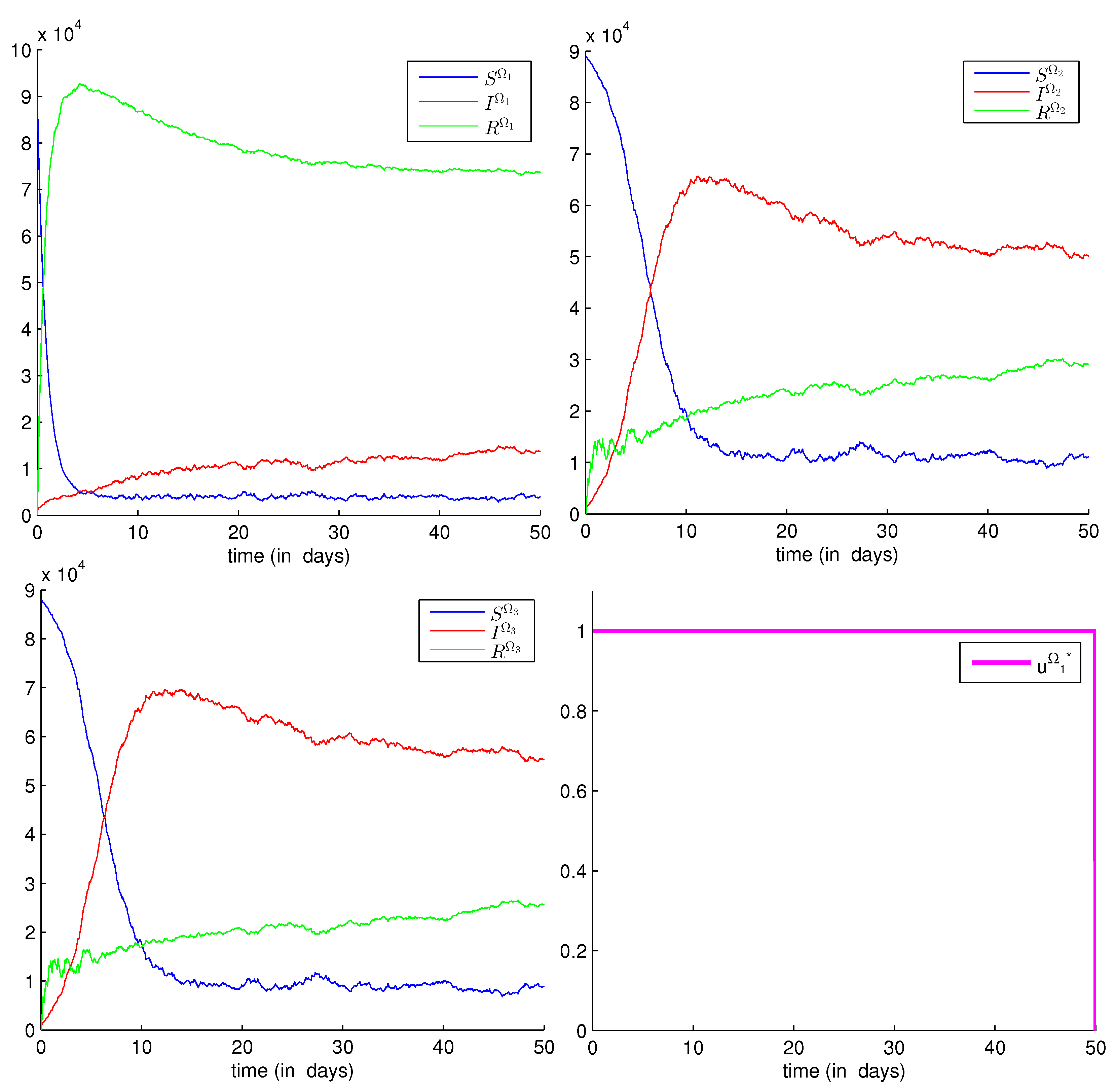
3.2.3. Numerical Results

In this part, we suppose we have three interconnected regions, and we investigate numerically using the stochastic progressive-regressive schemes method presented in [45] the effectiveness of the optimal control approach presented above. In our simulations, we note that:

-

We study three regions, denoted by ${\Omega }_1$, ${\Omega }_2$, and ${\Omega }_3$ and that are all assumed to be infected.

-

${\beta }_{jk}$ are replaced by ${\beta }_k$ just to avoid more complications in the program code. In other words, we assume that the probability to be infected does not depend on the source location of susceptibility, but on the source location of infectivity only, namely ${\Omega }_k$. More explicitly, ${\beta }_{11}={\beta }_{21}={\beta }_{31}$; they are represented by ${\beta }_1$, ${\beta }_{12}={\beta }_{22}={\beta }_{32}$; they are represented by ${\beta }_2$ and, finally, ${\beta }_{13}={\beta }_{23}={\beta }_{33}={\beta }_3$; and they are represented by ${\beta }_3$.

-

The unit of the parameters $d_j,{\gamma }_j$ and ${\beta }_{jk}$ is $day{s}^{-1}$∀ fixed j and mobile k.

-

$\forall i{t}_{i+1}=t_i+h,\Delta W_i\to \sqrt{h}N(0,1)$ with h the time step.

-

The coefficients in diffusions ${\delta }_j$, ${\varsigma }_{jk}$, and ${\sigma }_j$ are assumed to be all equal to 0.125. Larger values can be considered; however, they only increase the level of stochasticity, and this is not very interesting here.

Figure 1 depicts the dynamics of $S^{{\Omega }_j}$, $I^{{\Omega }_j}$, and $R^{{\Omega }_j}$, $j=1,2,3$ in the absence and presence of optimal controls $u^{{\Omega }_1*},u^{{\Omega }_2*}$, and $u^{{\Omega }_3*}$. As we can observe in the upper part of this figure and because of a strong immunity of a fraction of the population, there is a natural recovery from the infection and that causes an increase of the number of $R^{{\Omega }_j}$ in all three regions, but without exceeding the number of 40,000 people.

In the same part, we can also see that the number of infected people, namely $I^{{\Omega }_j}\forall j$, exceeds 70,000 people, and this proves the necessity of an urgent control measure to fight against the epidemic. In the lower part of this figure, we reach our goal that is summarized in maximizing the number of removed people while minimizing the number of infected people, and we can observe that the number of removed individuals has reached now a number that is near 90,000 people in all regions, while the number of infected people tended to zero values after 30, 40, and 48 days in regions ${\Omega }_1$, ${\Omega }_2$, and ${\Omega }_3$, respectively. We note that the optimal controls $u^{{\Omega }_j*},\forall j$ take the same values along the optimal control strategy period and that are all equal to one, and they tend to zero at the final time T. This is also the reason behind our avoidance of exhibiting simulations of the three optimal controls separately.

In Figure 2, we deduce that when we follow the optimal vaccination control strategy in the two regions ${\Omega }_2$ and ${\Omega }_3$, the number $R^{{\Omega }_j},j=2,3$ exceeded 100,000 individuals in the first five days, but decreased after towards values around 80,000 people, which represents an important value also, but they were smaller values than the ones obtained in the case treated in the first figure. In addition, the number $I^{{\Omega }_j},j=2,3$ decreased to values around 2000 people, which shows also the effectiveness of the followed vaccination control strategy, but they were larger values than the ones obtained in the previous case. In parallel, despite the cancellation of vaccination in region ${\Omega }_1$, we can see that the number of removed people approached values around 50,000, which shows an increase by 10,000 people compared to the case when controls were not introduced in all regions, and this proves some influence of the optimal control policy followed in other regions in a region that is not yet controlled directly. We note also here that the optimal controls $u^{{\Omega }_j*},j=2,3$ take the same values along the optimal control strategy period, which were all equal to one with some perturbations after 5 days, and they tended to zero at the final time T.

In Figure 3, we study the dynamics of $S^{{\Omega }_j}$, $I^{{\Omega }_j}$, and $R^{{\Omega }_j},j=1,2,3$ when we introduce an optimal vaccination control in region ${\Omega }_1$ only, and we can deduce some negative impact of the two regions ${\Omega }_2$ and ${\Omega }_3$ on the first region due to the absence of a control strategy in them. In fact, as they were at higher risk of infection than region ${\Omega }_1$, the optimal control $u^{{\Omega }_1*}$ seemed not sufficient for eradicating infection, as shown in first figure when controls were introduced in all regions, but this can at least increase the number of removed people in this region to an important value that exceeds 90,000 individuals. We note that the optimal control $u^{{\Omega }_1*}$ takes one as the maximal value.

4. The Model with Vaccination Plus Movement Restriction

4.1. Presentation of the Control Model

Let $I=\left\{1,...,p\right\}$ and $I_H\subset I$ be the set of indices of regions at high-risk and then having the ability to spread the epidemic to other regions. Here, we study the case when a given region ${\Omega }_j$ is under vaccination control $u^{{\Omega }_j}$ and at the same time under the threat of infection coming from other regions. For this, we add to the vaccination strategy another control denoted as $v^{j{\Omega }_k}$ to characterize the effectiveness of movement restriction operations, in order to prevent the infected of regions ${\Omega }_k,k\in I_H$ coming to the controlled region ${\Omega }_j$, where:

$$\left\{\begin{array}{ccc}{v}^{j{\Omega }_k}\ne 0& \forall k\in I_H& k\ne j\\ v^{j{\Omega }_k}=0& \mathrm{elsewhere}\end{array}\right.$$

(23)

Then, the model (24)–(26) in the controlled region ${\Omega }_j$ is rewritten as follows:

$$\begin{array}{ccc}\hfill {\dot{S}}^{{\Omega }_j}\left(t\right)& =-& \begin{array}{c}{\displaystyle \sum _{k=1}^p}\end{array}{\vartheta }^{jk}\left(t\right)\frac{I^{{\Omega }_k}\left(t\right)}{N^{{\Omega }_j}\left(t\right)}{S}^{{\Omega }_j}\left(t\right)+\left(N^{{\Omega }_j}\left(t\right)-S^{{\Omega }_j}\left(t\right)\right)d_j\hfill \\ & & -{\theta }^{{\Omega }_j}\left(t\right)S^{{\Omega }_j}\left(t\right)\hfill \end{array}$$

(24)

$$\begin{array}{ccc}\hfill {\dot{I}}^{{\Omega }_j}\left(t\right)& =& \begin{array}{c}{\displaystyle \sum _{k=1}^p}\end{array}{\vartheta }^{jk}\left(t\right)\frac{I^{{\Omega }_k}\left(t\right)}{N^{{\Omega }_j}\left(t\right)}{S}^{{\Omega }_j}\left(t\right)-{\gamma }_j{I}^{{\Omega }_j}\left(t\right)-d_j{I}^{{\Omega }_j}\left(t\right)\hfill \\ \hfill \end{array}$$

(25)

$$\begin{array}{ccc}\hfill {\dot{R}}^{{\Omega }_j}\left(t\right)& =& {\gamma }_j{I}^{{\Omega }_j}\left(t\right)-d_j{R}^{{\Omega }_j}\left(t\right)+{\theta }^{{\Omega }_j}\left(t\right)S^{{\Omega }_j}\left(t\right)\hfill \end{array}$$

(26)

with the vaccination control defined as:

$${\displaystyle {\theta }^{{\Omega }_j}\left(t\right)=u^{{\Omega }_j}\left(t\right)+{\delta }_j\frac{d{W}^{{\Omega }_j}\left(t\right)}{dt}.}$$

and the function ${\vartheta }^{jk}\left(t\right)$ defined as:

$${\vartheta }^{jk}\left(t\right)=\left(1-v^{j{\Omega }_k}\right){\beta }_{jk}+(1-{\varsigma }_{jk}){\sigma }_j\frac{d{W}^{{\Omega }_j}\left(t\right)}{dt}$$

where ${\sigma }_j$ and ${\varsigma }_{jk}$, $k\in I_H$, $(j=1,\dots ,p)$ are real constants and representing the intensities of fluctuations caused by media and escapes of infected people through borders between ${\Omega }_k$ and ${\Omega }_j$, respectively.

4.2. A Stochastic Optimal Control Approach

Now, the problem (Section 3.2.1) is changed in this part to

${\displaystyle J(u^{{\Omega }_j},v^{j\Omega })=\sum _{k\in I_H}\mathbb{E}\left({\displaystyle {\int }_0^T\left({\alpha }_j^I{I}^{{\Omega }_j}\left(t\right)-{\alpha }_j^R{R}^{{\Omega }_j}\left(t\right)+\frac{A_j}{2}{\left(u^{{\Omega }_j}\left(t\right)\right)}^2+\frac{B_j}{2}{\left(v^{j{\Omega }_k}\left(t\right)\right)}^2\right)dt}\right)}$ where $B_j>0$ is the weight constant of the new control, while $u^{{\Omega }_j}\in U_j$ and $v^{j\Omega }={\left(v^{j{\Omega }_k}\right)}_{k\in I_H}$ belong to the control set $V_j^{I_H}$ defined as:

$$V_j^{I_H}\left([0,T]\right)=\{v^{j\Omega }\left(t\right){\mathcal{F}}_t-progressivelymeasurable|v_{min}^{{\Omega }_j}\le v^{j{\Omega }_k}\left(t\right)\le v_{max}^{{\Omega }_j},k\in I_H,t\in [0,T]\}$$

The Hamiltonian in this case is defined as:

$$\begin{array}{ccc}\hfill H& =& {\displaystyle \sum _{k\in I_H}\left({\alpha }_j^I{I}^{{\Omega }_j}\left(t\right)-{\alpha }_j^R{R}^{{\Omega }_j}\left(t\right)+\frac{A_j}{2}{\left(u^{{\Omega }_j}\left(t\right)\right)}^2+\frac{B_j}{2}{\left(v^{j{\Omega }_k}\left(t\right)\right)}^2+{\mu }^{{\Omega }_j^T}\left(t\right)f(t,x^{{\Omega }_j}\left(t\right),u^{{\Omega }_j}\left(t\right),v^{j{\Omega }_k}\left(t\right))\right.}\hfill \\ & +& \left.{\displaystyle \sum _{l=1}^3{g}^{l^T}(x^{{\Omega }_j}\left(t\right),u^{{\Omega }_j}\left(t\right),v^{j{\Omega }_k}\left(t\right)){\nu }^{{\Omega }_j^l}\left(t\right)}\right)\hfill \end{array}$$

where the state function f is defined as:

$f(t,x^{\Omega }\left(t\right),u^{\Omega }\left(t\right),v^{j\Omega }\left(t\right))$

$$=\left(\begin{array}{c}{\displaystyle -\sum _{k=1}^p\left(1-v^{j{\Omega }_k}\right){\beta }_{jk}\frac{I^{{\Omega }_k}\left(t\right)}{N^{{\Omega }_j}\left(t\right)}{S}^{{\Omega }_j}\left(t\right)+\left(N^{{\Omega }_j}\left(t\right)-S^{{\Omega }_j}\left(t\right)\right)d_j-u^{{\Omega }_j}\left(t\right)S^{{\Omega }_j}\left(t\right)}\\ {\displaystyle \sum _{k=1}^p\left(1-v^{j{\Omega }_k}\right){\beta }_{jk}\frac{I^{{\Omega }_k}\left(t\right)}{N^{{\Omega }_j}\left(t\right)}{S}^{{\Omega }_j}\left(t\right)-{\gamma }_j{I}^{{\Omega }_j}\left(t\right)-d_j{I}^{{\Omega }_j}\left(t\right)}\\ {\gamma }_j{I}^{{\Omega }_j}\left(t\right)-d_j{R}^{{\Omega }_j}\left(t\right)+u^{{\Omega }_j}\left(t\right)S^{{\Omega }_j}\left(t\right)\end{array}\right)$$

and the diffusion matrix g is defined as:

$$g(t,x^{\Omega }\left(t\right),u^{\Omega }\left(t\right),v^{j\Omega }\left(t\right))=\left(\begin{array}{c}-\left({\displaystyle {\sigma }_j\sum _{k=1}^p(1-{\varsigma }_{jk})\frac{I^{{\Omega }_k}\left(t\right)}{N^{{\Omega }_j}\left(t\right)}{S}^{{\Omega }_j}\left(t\right)+{\delta }_j{S}^{{\Omega }_j}\left(t\right)}\right)\\ {\displaystyle {\sigma }_j\sum _{k=1}^p(1-{\varsigma }_{jk})\frac{I^{{\Omega }_k}\left(t\right)}{N^{{\Omega }_j}\left(t\right)}{S}^{{\Omega }_j}\left(t\right)}\\ {\delta }_j{S}^{{\Omega }_j}\left(t\right)\end{array}\right)$$

while in a domain $\Omega$, $\left(\mu \right(t),\nu (t\left)\right)$) is a pair of adjoint variables satisfying the following adjoint BSDE (backward stochastic differential equation):

$$\begin{array}{c}\hfill \left\{\begin{array}{ccc}\hfill d{\mu }^{\Omega }\left(t\right)& =& -[f_x^T(t,x^{\Omega }\left(t\right),u^{\Omega }\left(t\right),v^{j\Omega }\left(t\right)){\mu }^{\Omega }\left(t\right)+\sum _{l=1}^3{g}_{x^{\Omega }}^{l^T}(t,x^{\Omega }\left(t\right),u^{\Omega }\left(t\right),v^{j\Omega }\left(t\right)){\nu }^{{\Omega }^l}\left(t\right)\hfill \\ & & +f_{0_{x^{\Omega }}}(t,x^{\Omega }\left(t\right),u^{\Omega }\left(t\right),v^{j\Omega }\left(t\right))]dt+{\nu }^{\Omega }\left(t\right)d{W}^{\Omega }\left(t\right),\hfill \\ \hfill {\mu }^{\Omega }\left(T\right)& =& 0.\hfill \end{array}\right.\end{array}$$

(27)

4.2.1. Optimal Control Characterization and Necessary Conditions

Using the stochastic Pontryagin’s maximum principle as done for the first control strategy, we obtain the following optimal control characterization and necessary conditions:

Theorem 2.

If there exists an optimal pair $(x^{\Omega *},u^{\Omega *},v^{j\Omega *})$ and a pair of processes $\left(\mu \right(t),\nu (t\left)\right)$ satisfying (27), then for $j=1,...,p$, $k\in I_H$, we have:

$$H(t,x^{{\Omega }_j*}\left(t\right),u^{{\Omega }_j*}\left(t\right),v^{j{\Omega }_k*}\left(t\right),{\mu }^{{\Omega }_j}\left(t\right),{\nu }^{{\Omega }_j}\left(t\right))$$

$$=\underset{(u^{{\Omega }_j},v^{j{\Omega }_k}\left(t\right))\in U_j\times V_j^{I_H}}{min}H(t,x^{{\Omega }_j}\left(t\right),u^{{\Omega }_j*}\left(t\right),v^{j{\Omega }_k*}\left(t\right),{\mu }^{{\Omega }_j}\left(t\right),{\nu }^{{\Omega }_j}\left(t\right)).$$

Moreover, we obtain the bounded stochastic control:

$${\displaystyle u^{{\Omega }_j*}=min(max(u_{min}^{{\Omega }_j},-\frac{({\mu }_3^{{\Omega }_j}\left(t\right)-{\mu }_1^{{\Omega }_j}\left(t\right))S^{{\Omega }_j*}}{A_j}),u_{max}^{{\Omega }_j}),}$$

$${\displaystyle v^{j{\Omega }_k*}=min(max(v_{min}^{{\Omega }_j},-\frac{({\mu }_1^{{\Omega }_j}\left(t\right)-{\mu }_2^{{\Omega }_j}\left(t\right)){\beta }_{jk}{I}^{{\Omega }_k*}{S}^{{\Omega }_j*}}{B_j}),v_{max}^{{\Omega }_j}),}$$

and solutions of the FBSDEs (forward-backward stochastic differential equations):

$$\begin{array}{c}\hfill \left\{\begin{array}{ccc}d{x}^{{\Omega }_j}\left(t\right)\hfill & =\hfill & f(t,x^{{\Omega }_j}\left(t\right),u^{{\Omega }_j}\left(t\right),v^{j{\Omega }_k}\left(t\right))dt+g(t,x^{{\Omega }_j}\left(t\right),u^{{\Omega }_j}\left(t\right),v^{j{\Omega }_k}\left(t\right))d{W}^{{\Omega }_j}\left(t\right)\hfill \\ d{\mu }^{{\Omega }_j}\left(t\right)\hfill & =\hfill & -[f_{x^{{\Omega }_j}}^T(t,x^{{\Omega }_j}\left(t\right),u^{{\Omega }_j}\left(t\right),v^{j{\Omega }_k}\left(t\right)){\mu }^{{\Omega }_j}\left(t\right)+\sum _{l=1}^3{g}_{x^{{\Omega }_j}}^{l^T}(t,x^{{\Omega }_j}\left(t\right),u^{{\Omega }_j}\left(t\right),v^{j{\Omega }_k}\left(t\right)){\nu }^{{\Omega }_j^l}\left(t\right)\hfill \\ & & +f_{0_{x^{{\Omega }_j}}}(t,x^{{\Omega }_j}\left(t\right),u^{{\Omega }_j}\left(t\right),v^{j{\Omega }_k}\left(t\right))]dt+{\nu }^{{\Omega }_j}\left(t\right)d{W}^{{\Omega }_j}\left(t\right),\hfill \\ x^{{\Omega }_j}\left(0\right)\hfill & =\hfill & (S_0^{{\Omega }_j},I_0^{{\Omega }_j},R_0^{{\Omega }_j})\hfill \\ {\mu }^{{\Omega }_j}\left(T\right)\hfill & =\hfill & 0.\hfill \end{array}\right.\end{array}$$

(28)

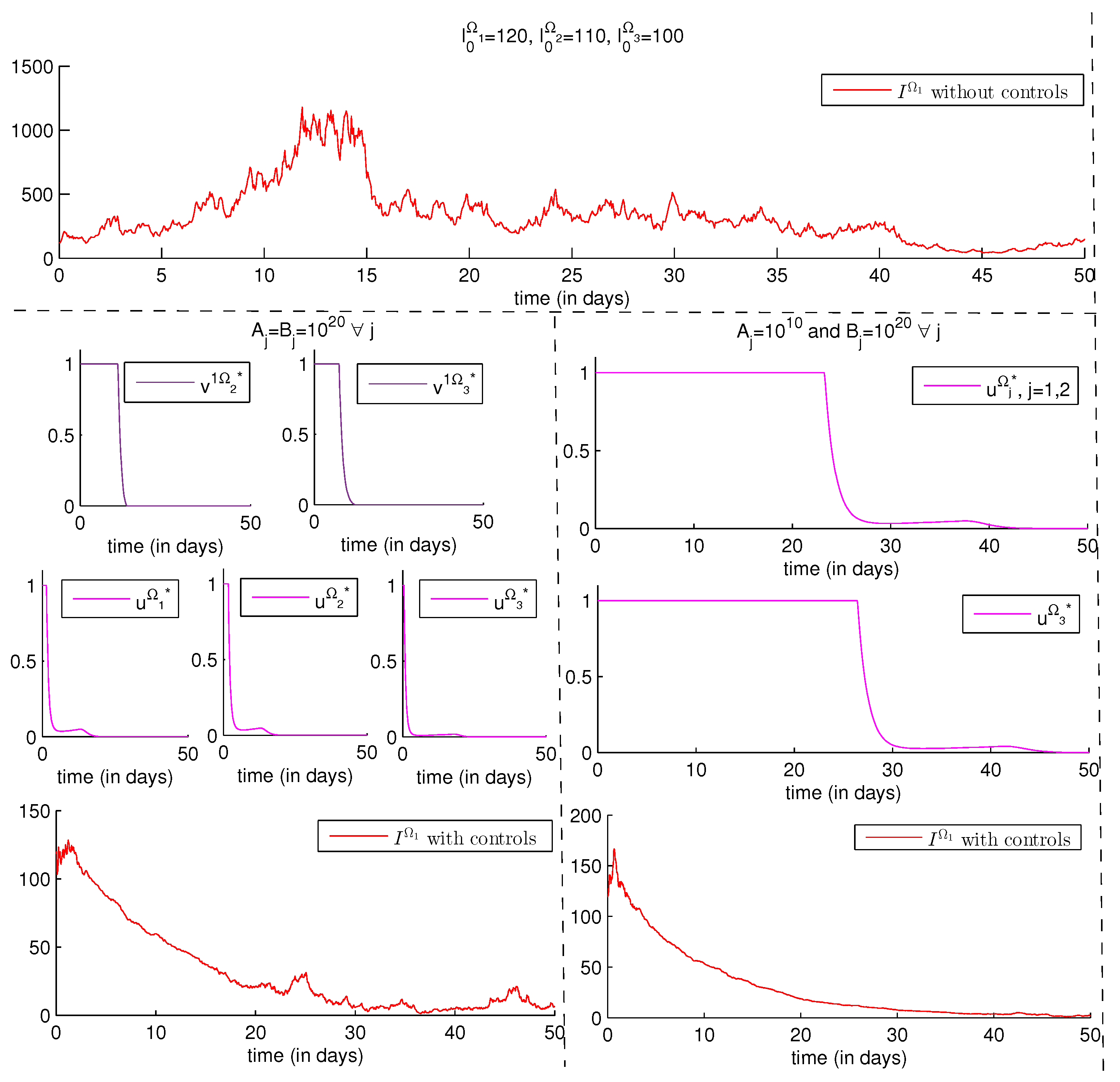
4.2.2. Numerical Results

In this part, we show the importance of following an optimal control strategy that is based on movement restrictions along with the presence of the vaccination policy discussed previously. For this, we take the example of preventing the epidemic from arriving at the region ${\Omega }_1$ through infected travelers who come from other regions. This means we restrict movements of infected people coming from ${\Omega }_2$ and ${\Omega }_3$ either using $v^{1{\Omega }_2*}$ and/or $v^{1{\Omega }_3*}$, respectively. Figure 4 presents the simulations of $I^{{\Omega }_j}$ and $R^{{\Omega }_j},j=1,2,3$ in the presence of all optimal controls $u^{{\Omega }_1*},u^{{\Omega }_2*}$, and $u^{{\Omega }_3*}$, and we can see that when we restrict movement of individuals coming from region ${\Omega }_2$ and aiming to enter ${\Omega }_1$, we can reach smaller values of infected people after only 15 days in all regions; at the same time, we deduce that the level of the number of removed people is approximately the same as in the absence of movement restrictions. We note that the optimal controls $u^{{\Omega }_j*},j=2,3$ along with the optimal control $v^{1{\Omega }_2*}$ take the same values along the optimal control strategy period, which are all equal to one, and they tend to zero at the final time T.

In Figure 5, we can better see the importance of movement restrictions, especially when we prevent also individuals coming from region ${\Omega }_3$, which is at highest risk of infection. In fact, when we add the optimal control $v^{1{\Omega }_2*}$ to $v^{1{\Omega }_3*}$, we can reach better results as in the previous case since the number of infected people has decreased more and the number of removed people has increased more in all regions compared to the case when optimal controls $u^{{\Omega }_1*},u^{{\Omega }_2*}$, and $u^{{\Omega }_3*}$ are followed alone. We note also here that the optimal controls $u^{{\Omega }_j*},j=2,3$ along with the optimal controls $v^{1{\Omega }_k*},k=2,3$ take the same values along the optimal control strategy period, which are all equal to one, and they tend to zero at the final time T.

5. Discussion

In this section, we provide other simulations to compare between the results of the optimal control strategy proposed in Section 3 and the other one treated in Section 4, as well as the case when there was no control yet as defined in Section 1. We also discuss the effect of severity controls weight $A_j$ and $B_j$ and the initial conditions of infection on the optimal values of controls and states.

In Figure 6, we treat the case when there is no vaccination in region ${\Omega }_1$, and we compare it with the case when there is no control policy in all regions and with the case treated in Figure 1. From this figure, we can deduce that even in the absence of vaccination in the first region, there is an advantage of movement restrictions represented by optimal controls $v^{1{\Omega }_k*},k=2,3$, applied between region ${\Omega }_1$ and other regions, in decreasing the number of infected people and increasing the number of removed people. This figure also shows the importance of vaccination when it is followed in all regions, and that can be strengthened more if we add $v^{1{\Omega }_k*},k=2,3$, as concluded in the previous figure. We note also here that the optimal controls $u^{{\Omega }_j*},j=1,2,3$ along with the optimal controls $v^{1{\Omega }_k*},k=2,3$ take the same values along the optimal control strategy period, which are all equal to one, with some perturbations after five days, and they tend to zero at the final time T.

As in Figure 7, we present the simulation of the function $I^{{\Omega }_1}$ when there is no control, and we compare it with the case with the control for different values of severity controls weights, namely $A_j$ and $B_j$ associated with $u^{{\Omega }_j*}$ and $v^{j{\Omega }_k*}$, respectively, as noted previously. We observe that after introducing the five optimal controls $u^{{\Omega }_j*},j=1,2,3$, $v^{1{\Omega }_2*}$, and $v^{1{\Omega }_3*}$, the number of infected people has decreased towards the value of 400 individuals when $A_j=1$, referring to the previous cases for obtaining $u^{{\Omega }_j*}$, but with $B_j={10}^{20}$ now. This number can be decreased earlier, as we can see below in the left-hand side part of this figure when we take $A_j={10}^4$. Defined as the denominator in the characterization of $v^{j{\Omega }_k*}$, the value $B_j={10}^{20}$ here implies a reduction of the optimal controls’ values, $v^{1{\Omega }_2*}$ and $v^{1{\Omega }_3*}$, and the movement restriction is recommended for the first 22 and 25 days only. However, when we give a less important value to $B_j$, ${10}^8$ for example, we can observe that a long period of this strategy minimized the function $I^{{\Omega }_1}$ more significantly, and it can be minimized and even earlier than this when we take $A_j=B_j={10}^4$, as seen below in the right-hand side of the figure.

As the last Figure 8, we are interested in doing the same as in the previous figure, but in the case of less important values for initial conditions $I_0^{{\Omega }_j},j=1,2,3$ and smaller values for optimal controls $u^{{\Omega }_j*},j=1,2,3$, $v^{1{\Omega }_2*}$, and $v^{1{\Omega }_3*}$. From this figure, we observe that when there is no control, the function $I^{{\Omega }_1}$ does not increase to larger values as observed in the first figures, and then, we understand that we will not need to vaccinate everyone and close all borders for all times of the control strategy period. As predicted, we observe that when we add the value ${10}^{20}$ to both denominators $A_j$ and $B_j$, implying an important reduction of all optimal controls, the number of infected people in ${\Omega }_1$ decreased to very small values after 20 days only, and this can be done more effectively when vaccination is prolonged, as we can observe in the right-hand side of the figure, when we add ${10}^{10}$ to $A_j$.

6. Conclusions

In this paper, we have proposed a stochastic model for the study of infection dynamics when an epidemic emerges in regions that are connected by any kind of anthropological movement, considering perturbations that are due to media, infodemics, and escapes. We have also suggested two optimal control approaches related to vaccination and movement restriction policies based on a stochastic version of Pontryagin’s maximum principle.

References

1. Liu, R.; Wu, J.; Zhu, H. Media/psychological impact on multiple outbreaks of emerging infectious diseases. Comput. Math. Methods Med. 2007, 8, 153–164. [Google Scholar] [CrossRef]
2. Sahu, G.P.; Dhar, J. Dynamics of an SEQIHRS epidemic model with media coverage, quarantine and isolation in a community with pre-existing immunity. J. Math. Anal. Appl. 2015, 421, 1651–1672. [Google Scholar] [CrossRef]
3. Wang, A.; Xiao, Y. A Filippov system describing media effects on the spread of infectious diseases. Nonlinear Anal. Hybrid Syst. 2014, 11, 84–97. [Google Scholar] [CrossRef]
4. Liu, Y.; Cui, J.A. The impact of media coverage on the dynamics of infectious disease. Int. J. Biomath. 2008, 1, 65–74. [Google Scholar] [CrossRef]
5. Samanta, S.; Rana, S.; Sharma, A.; Misra, A.K.; Chattopadhyay, J. Effect of awareness programs by media on the epidemic outbreaks: A mathematical model. Appl. Math. Comput. 2013, 219, 6965–6977. [Google Scholar] [CrossRef]
6. Misra, A.K.; Sharma, A.; Shukla, J.B. Stability analysis and optimal control of an epidemic model with awareness programs by media. Biosystems 2015, 138, 53–62. [Google Scholar] [CrossRef]
7. Yuan, X.; Xue, Y.; Liu, M. Analysis of an epidemic model with awareness programs by media on complex networks. Chaos Solitons Fractals 2013, 48, 1–11. [Google Scholar] [CrossRef]
8. Wang, Y.; Cao, J.; Jin, Z.; Zhang, H.; Sun, G.Q. Impact of media coverage on epidemic spreading in complex networks. Phys. A Stat. Mech. Its Appl. 2013, 392, 5824–5835. [Google Scholar] [CrossRef]
9. World Health Organization. Managing Epidemics: Key Facts About Major Deadly Diseases; World Health Organization: Geneva, Switzerland, 2018. [Google Scholar]
10. Zakary, O.; Larrache, A.; Rachik, M.; Elmouki, I. Effect of awareness programs and travel-blocking operations in the control of HIV/AIDS outbreaks: A multi-domains SIR model. Adv. Differ. Equ. 2016, 2016, 169. [Google Scholar] [CrossRef]
11. Zakary, O.; Rachik, M.; Elmouki, I. A multi-regional epidemic model for controlling the spread of Ebola: Awareness, treatment, and travel-blocking optimal control approaches. Math. Methods Appl. Sci. 2017, 40, 1265–1279. [Google Scholar] [CrossRef]
12. Zakary, O.; Rachik, M.; Elmouki, I. On the analysis of a multi-regions discrete SIR epidemic model: An optimal control approach. Int. J. Dyn. Control 2017, 5, 917–930. [Google Scholar] [CrossRef]
13. Zakary, O.; Rachik, M.; Elmouki, I. A new analysis of infection dynamics: Multi-regions discrete epidemic model with an extended optimal control approach. Int. J. Dyn. Control 2017, 5, 1010–1019. [Google Scholar] [CrossRef]
14. Abouelkheir, I.; El Kihal, F.; Rachik, M.; Zakary, O.; Elmouki, I. A multi-regions SIRS discrete epidemic model with a travel-blocking vicinity optimal control approach on cells. Br. J. Math. Comput. Sci. 2017, 20, 1–16. [Google Scholar] [CrossRef] [PubMed]
15. El Kihal, F.; Rachik, M.; Zakary, O.; Elmouki, I. A multi-regions SEIRS discrete epidemic model with a travel-blocking vicinity optimal control approach on cells. Int. J. Adv. Appl. Math. Mech. 2017, 4, 60–71. [Google Scholar]
16. Abouelkheir, I.; Rachik, M.; Zakary, O.; Elmouki, I. A multi-regions SIS discrete influenza pandemic model with a travel-blocking vicinity optimal control approach on cells. Am. J. Comput. Appl. Math. 2017, 7, 37–45. [Google Scholar]
17. Zakary, O.; Rachik, M.; Elmouki, I.; Lazaiz, S. A multi-regions discrete-time epidemic model with a travel-blocking vicinity optimal control approach on patches. Adv. Differ. Equ. 2017, 2017, 120. [Google Scholar] [CrossRef]
18. Chouayakh, K.; Rachik, M.; Zakary, O.; Elmouki, I. A multi-regions SEIS discrete epidemic model with a travel-blocking vicinity optimal control approach on cells. J. Math. Comput. Sci. 2017, 7, 468–484. [Google Scholar]
19. Zakary, O.; Rachik, M.; Elmouki, I. A new epidemic modeling approach: Multi-regions discrete-time model with travel-blocking vicinity optimal control strategy. Infect. Dis. Model. 2017, 2, 304–322. [Google Scholar] [CrossRef] [PubMed]
20. Bidah, S.; Rachik, M.; Zakary, O.; Boutayeb, H.; Elmouki, I. Travel-blocking Optimal Control Policy on Borders of a Chain of Regions Subject to SIRS Discrete Epidemic Model. Asian J. Res. Infect. Dis. 2018, 1, 1–12. [Google Scholar]
21. Zakary, O.; Bidah, S.; Rachik, M.; Elmouki, I. Cell and patch vicinity travel restrictions in a multi-regions SI discrete epidemic control model. Int. J. Adv. Appl. Math. Mech. 2019, 6, 30–41. [Google Scholar]
22. Zhang, X.B.; Huo, H.F.; Xiang, H.; Meng, X.Y. Dynamics of the deterministic and stochastic SIQS epidemic model with non-linear incidence. Appl. Math. Comput. 2014, 243, 546–558. [Google Scholar] [CrossRef]
23. Ji, C.; Jiang, D. Threshold behaviour of a stochastic SIR model. Appl. Math. Model. 2014, 38, 5067–5079. [Google Scholar] [CrossRef]
24. Ji, C.; Jiang, D.; Shi, N. The behavior of an SIR epidemic model with stochastic perturbation. Stoch. Anal. Appl. 2012, 30, 755–773. [Google Scholar] [CrossRef]
25. Jiang, D.; Ji, C.; Shi, N.; Yu, J. The long time behavior of DI SIR epidemic model with stochastic perturbation. J. Math. Anal. Appl. 2010, 372, 162–180. [Google Scholar] [CrossRef] [Green Version]
26. Liu, W. A SIRS epidemic model incorporating media coverage with random perturbation. In Abstract and Applied Analysis; Hindawi: Cairo, Egypt, 2013; Volume 2013. [Google Scholar]
27. Cai, Y.; Wang, X.; Wang, W.; Zhao, M. Stochastic dynamics of an SIRS epidemic model with ratio-dependent incidence rate. In Abstract and Applied Analysis; Hindawi: Cairo, Egypt, 2013; Volume 2013. [Google Scholar]
28. Cai, Y.; Kang, Y.; Wang, W. A stochastic SIRS epidemic model with nonlinear incidence rate. Appl. Math. Comput. 2017, 305, 221–240. [Google Scholar] [CrossRef]
29. Cai, Y.; Kang, Y.; Banerjee, M.; Wang, W. A stochastic SIRS epidemic model with infectious force under intervention strategies. J. Differ. Equ. 2015, 259, 7463–7502. [Google Scholar] [CrossRef]
30. Zhao, Y.; Jiang, D. The threshold of a stochastic SIRS epidemic model with saturated incidence. Appl. Math. Lett. 2014, 34, 90–93. [Google Scholar] [CrossRef]
31. Zhao, Y.; Jiang, D. Dynamics of stochastically perturbed SIS epidemic model with vaccination. In Abstract and Applied Analysis; Hindawi: Cairo, Egypt, 2013; Volume 2013. [Google Scholar]
32. Zhao, Y.; Jiang, D.; O’Regan, D. The extinction and persistence of the stochastic SIS epidemic model with vaccination. Phys. A Stat. Mech. Its Appl. 2013, 392, 4916–4927. [Google Scholar] [CrossRef]
33. Lin, Y.; Jiang, D.; Wang, S. Stationary distribution of a stochastic SIS epidemic model with vaccination. Phys. A Stat. Mech. Its Appl. 2014, 394, 187–197. [Google Scholar] [CrossRef]
34. Witbooi, P.J. Stability of an SEIR epidemic model with independent stochastic perturbations. Phys. A Stat. Mech. Its Appl. 2013, 392, 4928–4936. [Google Scholar] [CrossRef] [Green Version]
35. Zhou, Y.; Zhang, W.; Yuan, S. Survival and stationary distribution of a SIR epidemic model with stochastic perturbations. Appl. Math. Comput. 2014, 244, 118–131. [Google Scholar] [CrossRef]
36. Gray, A.; Greenhalgh, D.; Hu, L.; Mao, X.; Pan, J. A stochastic differential equation SIS epidemic model. SIAM J. Appl. Math. 2011, 71, 876–902. [Google Scholar] [CrossRef]
37. Meng, X.; Zhao, S.; Feng, T.; Zhang, T. Dynamics of a novel nonlinear stochastic SIS epidemic model with double epidemic hypothesis. J. Math. Anal. Appl. 2016, 433, 227–242. [Google Scholar] [CrossRef]
38. Hethcote, H.W.; Waltman, P. Optimal vaccination schedules in a deterministic epidemic model. Math. Biosci. 1973, 18, 365–381. [Google Scholar] [CrossRef]
39. Yong, J.; Zhou, X.Y. Stochastic Controls Hamiltonian Systems and HJB equations. In Application of Mathematics; Springer: New York, NY, USA, 1999. [Google Scholar]
40. Bahlali, K.; Mezerdi, B.; Ouknine, Y. The maximum principle for optimal control of diffusions with non-smooth coeffcients. Stoch. Stoch. Rep. 1996, 57, 303–316. [Google Scholar] [CrossRef]
41. Peng, S. A general stochastic maximum principle for optimal control problems. SIAM J. Control Optim. 1990, 28, 966–979. [Google Scholar] [CrossRef]
42. Ma, J.; Protter, P.; Yong, J. Solving Forward-Backward Stochastic Differential Equations Explicitly—A Four Step Scheme. J. Probab. Theory. Relat. Fields 1994, 98, 339–3359. [Google Scholar] [CrossRef]
43. Ladyz̆henskaia, O.A.; Solonnikov, V.A.; Ural’ceva, N.N. Linear and Quasi-Linear Equations of Parabolic Type; American Mathematical Soc.: Washington, DC, USA, 1968; Volume 23. [Google Scholar]
44. Düring, B.; Jüngel, A. Existence and uniqueness of solutions to a quasilinear parabolic equation with quadratic gradients in financial markets. Nonlinear Anal. Theory Methods Appl. 2005, 62, 519–544. [Google Scholar] [CrossRef]
45. Aboulaich, R.; Darouichi, A.; Elmouki, I.; Jraifi, A. A Stochastic Optimal Control Model for BCG Immunotherapy in Superficial Bladder Cancer. Math. Model. Nat. Phenom. 2017, 12, 99–119. [Google Scholar] [CrossRef]
Figure 1. (Top) S Ω j I Ω j R Ω j , j = 1 , 2 , 3 stochastic dynamics without controls. (Bottom) S Ω 1 I Ω 1 R Ω 1 stochastic dynamics in the presence of all optimal controls u Ω 1 * , u Ω 2 * , and u Ω 3 * . S 0 Ω 1 = 90,000, I 0 Ω 1 = 1200 , S 0 Ω 2 = 89,000, I 2 Ω 2 = 1100 , S 0 Ω 3 = 88,000, I 0 Ω 3 = 1000 , R 0 Ω j = 0 j = 1 , 2 , 3 , d 1 = 0 . 06 , γ 1 = 0 . 04 , β 1 = 0 . 5 , d 2 = 0 . 05 , γ 2 = 0 . 03 , β 2 = 0 . 4 , d 3 = 0 . 04 , γ 3 = 0 . 02 , β 3 = 0 . 1 .
Mathematics 07 00304 g001
Figure 2. S Ω j I Ω j R Ω j , j = 1 , 2 , 3 stochastic dynamics in the absence of optimal control u Ω 1 * and the presence of optimal controls u Ω 2 * and u Ω 3 * . Same parameters and initial conditions as in the first figure.
Mathematics 07 00304 g002
Figure 3. S Ω j I Ω j R Ω j , j = 1 , 2 , 3 stochastic dynamics in the absence of optimal controls u Ω 2 * and u Ω 3 * and the presence of optimal control u Ω 1 * only. S 0 Ω 1 = 90,000, I 0 Ω 1 = 1200 , S 0 Ω 2 = 89,000, I 2 Ω 2 = 1100 , S 0 Ω 3 = 88,000, I 0 Ω 3 = 1000 , R 0 Ω j = 0 j = 1 , 2 , 3 , d 1 = 0 . 06 , γ 1 = 0 . 04 , β 1 = 0 . 5 , d 2 = 0 . 05 , γ 2 = 0 . 03 , β 2 = 0 . 4 , d 3 = 0 . 04 , γ 3 = 0 . 02 , β 3 = 0 . 1 .
Mathematics 07 00304 g003
Figure 4. (Red and green curves) I Ω j and R Ω j , j = 1 , 2 , 3 dynamics with optimal controls u Ω 1 * , u Ω 2 * and u Ω 3 * . (Black curves) I Ω j and R Ω j , j = 1 , 2 , 3 dynamics with optimal controls u Ω 1 * , u Ω 2 * and u Ω 3 * plus v 1 Ω 2 * . S 0 Ω 1 = 90,000, I 0 Ω 1 = 1200 , S 0 Ω 2 = 89,000, I 2 Ω 2 = 1100 , S 0 Ω 3 = 88,000, I 0 Ω 3 = 1000 , R 0 Ω j = 0 j = 1 , 2 , 3 , d 1 = 0 . 06 , γ 1 = 0 . 04 , β 1 = 0 . 5 , d 2 = 0 . 05 , γ 2 = 0 . 03 , β 2 = 0 . 4 , d 3 = 0 . 04 , γ 3 = 0 . 02 , β 3 = 0 . 1 .
Mathematics 07 00304 g004
Figure 5. (Red and green curves) I Ω j and R Ω j , j = 1 , 2 , 3 dynamics with optimal controls u Ω 1 * , u Ω 2 * and u Ω 3 * . (Black curves) I Ω j and R Ω j , j = 1 , 2 , 3 dynamics with optimal controls u Ω 1 * , u Ω 2 * and u Ω 3 * plus v 1 Ω 2 * . S 0 Ω 1 = 90,000, I 0 Ω 1 = 1200 , S 0 Ω 2 = 89,000, I 2 Ω 2 = 1100 , S 0 Ω 3 = 88,000, I 0 Ω 3 = 1000 , R 0 Ω j = 0 j = 1 , 2 , 3 , d 1 = 0 . 06 , γ 1 = 0 . 04 , β 1 = 0 . 5 , d 2 = 0 . 05 , γ 2 = 0 . 03 , β 2 = 0 . 4 , d 3 = 0 . 04 , γ 3 = 0 . 02 , β 3 = 0 . 1 .
Mathematics 07 00304 g005
Figure 6. (Blue curves) I Ω j and R Ω j , j = 1 , 2 , 3 dynamics without controls. (Red and green curves) I Ω j and R Ω j , j = 1 , 2 , 3 dynamics with optimal controls u Ω 1 * , u Ω 2 * and u Ω 3 * . (Black curves) I Ω j and R Ω j , j = 1 , 2 , 3 dynamics with optimal controls u Ω 2 * and u Ω 3 * plus v 1 Ω 2 * . S 0 Ω 1 = 90,000, I 0 Ω 1 = 1200 , S 0 Ω 2 = 89,000, I 2 Ω 2 = 1100 , S 0 Ω 3 = 88,000, I 0 Ω 3 = 1000 , R 0 Ω j = 0 j = 1 , 2 , 3 , d 1 = 0 . 06 , γ 1 = 0 . 04 , β 1 = 0 . 5 , d 2 = 0 . 05 , γ 2 = 0 . 03 , β 2 = 0 . 4 , d 3 = 0 . 04 , γ 3 = 0 . 02 , β 3 = 0 . 1 .
Mathematics 07 00304 g006
Figure 7. I Ω 1 and optimal controls u Ω j * , j = 1 , 2 , 3 , v 1 Ω 2 * and v 1 Ω 3 * for different values of A j and B j .
Mathematics 07 00304 g007
Figure 8. I Ω 1 and optimal controls u Ω j * , j = 1 , 2 , 3 , v 1 Ω 2 * , and v 1 Ω 3 * for different values of A j and B j and less important initial condition of infection.
Mathematics 07 00304 g008