A New Parameter Estimator for the Generalized Pareto Distribution under the Peaks over Threshold Framework

Abstract
:1. Introduction
2. Estimation Methods
2.1. Peaks over Threshold
2.2. Existing Estimation Methods
2.2.1. Likelihood Moment Estimation
2.2.2. Maximum Likelihood Estimation
2.2.3. Weighted Nonlinear Least Squares Estimation
2.3. The Proposed Estimation Methods
2.3.1. Weighted Nonlinear Least Squares Moments Estimation
2.3.2. Weighted Nonlinear Least Squares Likelihood Moments Estimation
3. Simulation Studies
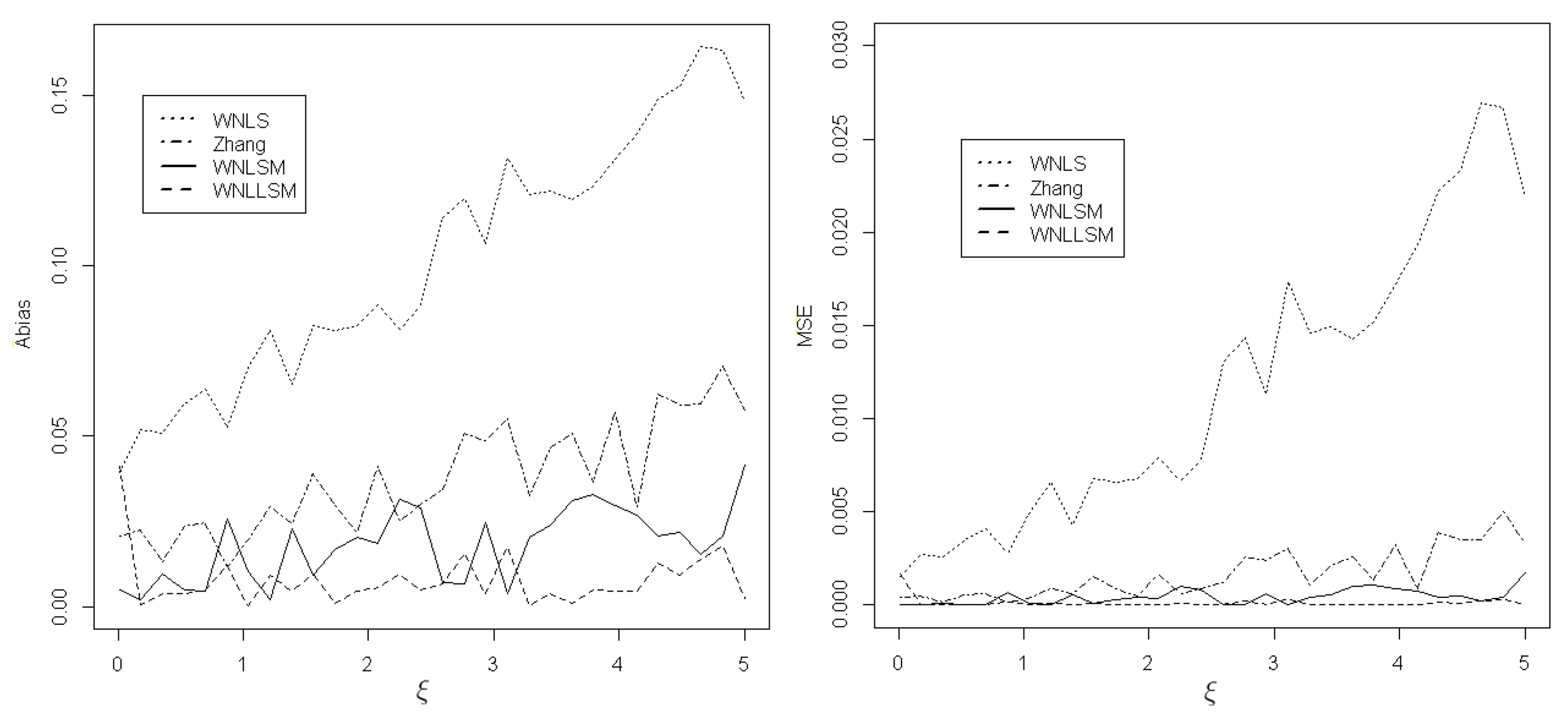
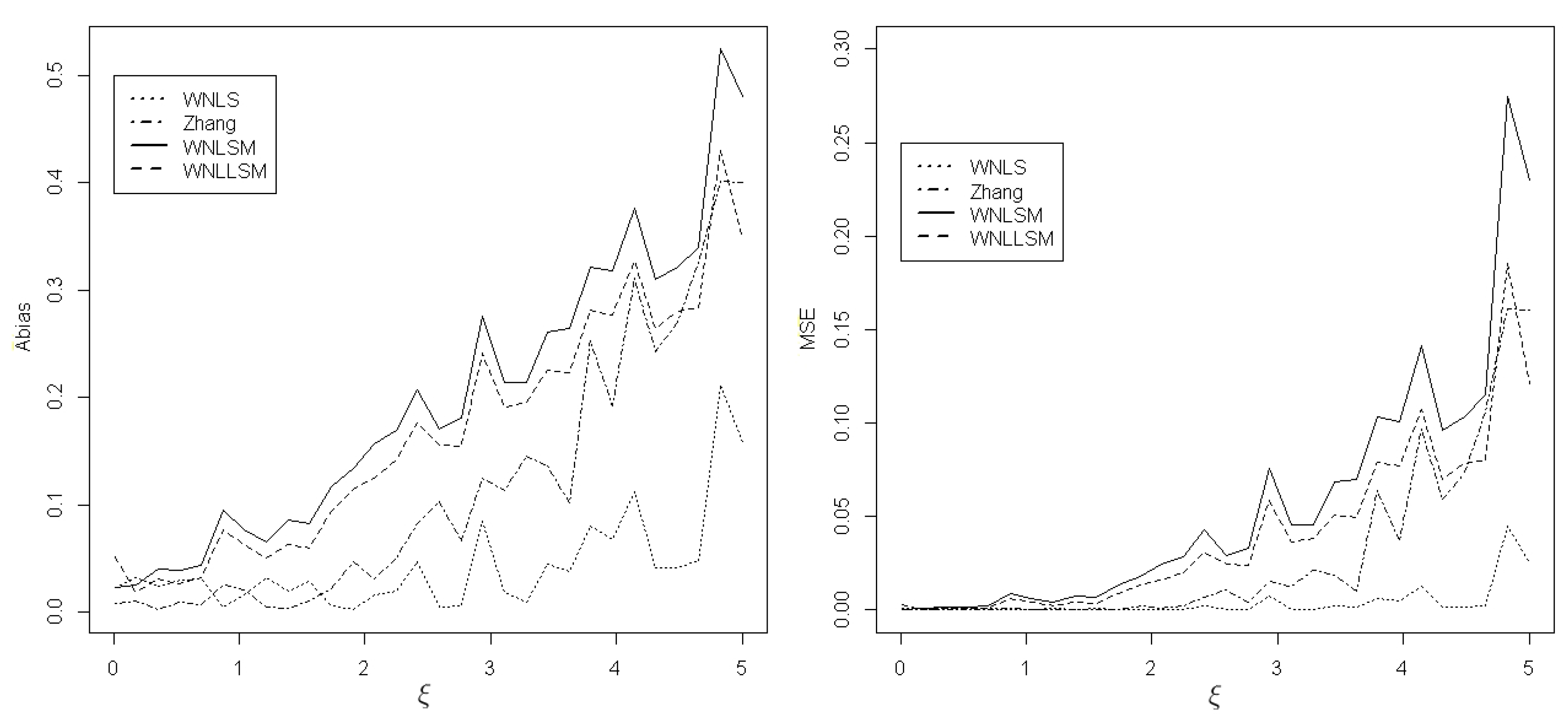
3.1. Simulation Study of the Parameter Estimation
- Generate i.i.d observations following the GPD(). We discuss the results for three different pairs of parameters under the GPD: () = (0.5, 1), (1, 10), and (2, 1).
- Use four methods to estimate , where .
- Repeat the above steps 100,000 times to compute the bias and MSE of estimators and b.
3.2. Simulation Study of the Threshold Selection
- (a)
- Fix , where i ranges from 1 to m, and m is a fixed positive integer.
- (b)
- Test proposed by [36], and compute the corresponding p-values .
- (c)
- Compute cutoff such thatwhere is a significance level. In this case, the selected threshold is .
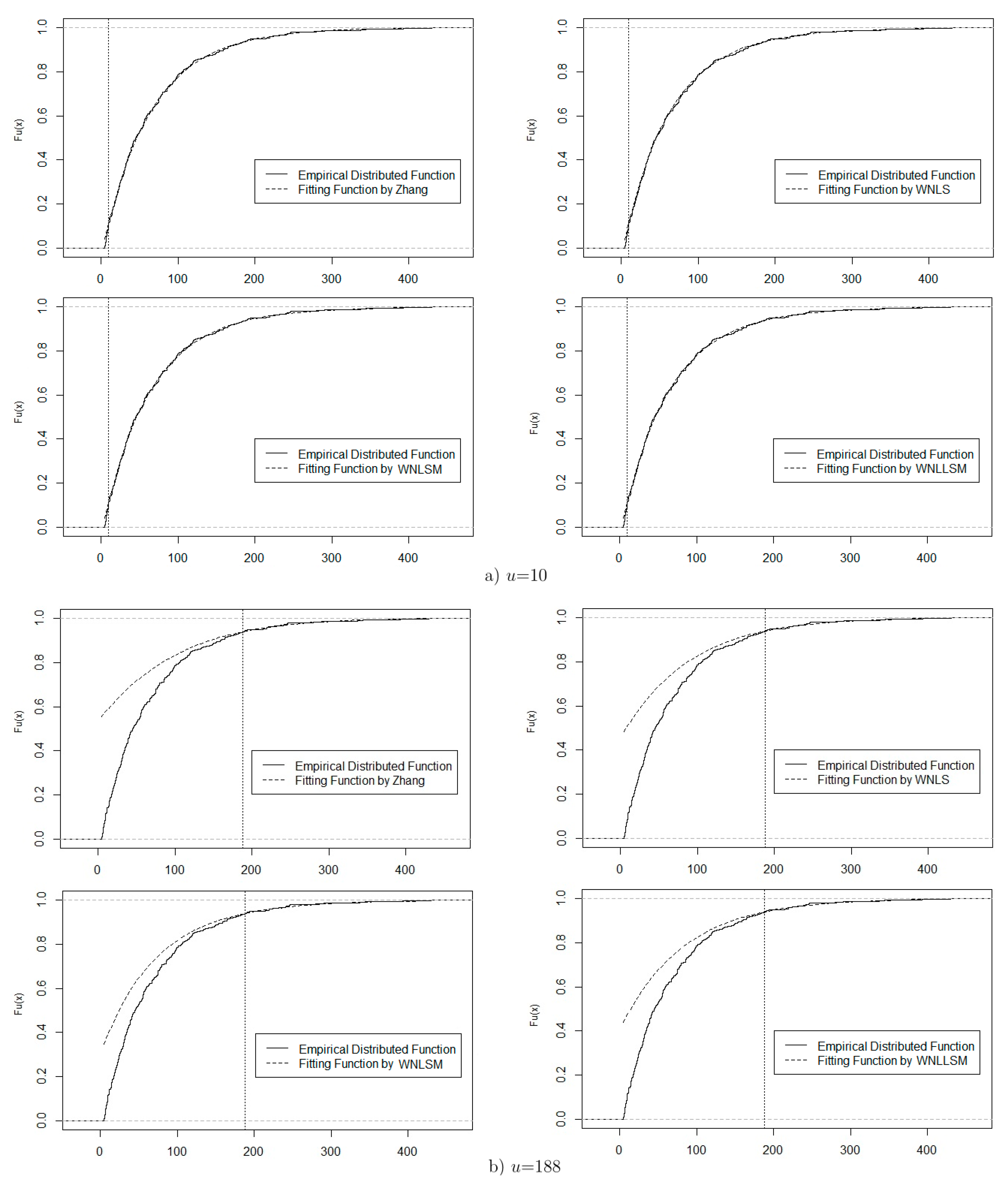
3.3. Application
- Use Raw Up, Raw Down, and ForwardStop rules to select the appropriate thresholds , , and , respectively.
- Obtain exceedances above the chosen threshold.
- Based on the exceedances, obtain parameter estimations of and by different methods.
4. Conclusions
Author Contributions
Funding
Acknowledgments
Conflicts of Interest
Appendix A
- #to estimate the weighted nonlinear least squares moments (WNLSM) of a
- sample X by GPD(xi, mu, sigma). For~the GPD, threshold u is equal to zero.
- sum_i <- function(i) sum(1/(n-seq(i)+1))
- WNLSM1 <- function(beta1){
- sum2 <- 0
- for (i in (nu0+1):n)
- { sum2 <- sum2 + (sum_i(i)+log(1-F0)-log(1+beta1[2]*(x[i]-u))/beta1[1]
- )^2 } #equation (10)
- sum2}
- #WNLSM1 searches for the initial WNLSM estimator (\hat(xi_1),\hat(b_1)),
- #where beta1=(xi, b), b=xi/sigma.
- WNLSM <- function(beta1){
- sum2 <- 0
- for (i in (nu0+1):n)
- {sum2 <- sum2 + ((n+1)^2*(n+2)/(i*(n-i+1)))*((i-n-1)/((n+1)*(1-F0))
- +(1+beta1[2]*(x[i]-u))^(-1/beta1[1]))^2} #equation (11)
- sum2}
- #WNLSM searches for the final WNLSM estimator (\hat(xi_2),\hat(b_2)).
- #to estimate the weighted nonlinear least squares likelihood moments
- (WNLLSM) of a sample X by GPD(xi, mu, sigma).
- WNLLSM1 <- function(b){
- sum1 <- mean(log(1+b*z))#z is the excess loss X-u|X>u and sum1=xi(b)
- #given in equation (4)
- sum2 <- 0
- for (i in (nu0+1):n){
- sum2 <- sum2 + (sum_i(i)+log(1-F0)-log(1+b*(x[i]-u))/sum1)^2}
- #equation (13)
- sum2}
- #WNLLSM1 searches for the initial WNLLSM estimator (\hat(xi_1),\hat(b_1)).
- WNLLSM <- function(b){
- sum1 <- mean(log(1+b*z)) #xi(b)
- sum2 <- 0
- for (i in (nu0+1):n){
- sum2 <- sum2 + ((n+1)^2*(n+2)/(i*(n-i+1)))*((i-n-1)/((n+1)*(1-F0))
- +(1+b*(x[i]-u))^(-1/sum1))^2} #equation (14)
- sum2}
- #WNLLSM searches for the final WNLLSM estimator (\hat(xi_2),\hat(b_2)).
- #Real data used in Section~3.3
References
- Ferreira, A.; de Haan, L. On the block maxima method in extreme value theory: PWM estimators. Ann. Stat. 2015, 43, 276–298. [Google Scholar] [CrossRef] [Green Version]
- Rolski, T.; Schmidli, H.; Schmidt, V.; Teugel, J. Stochastic Processes for Insurance and Finance; John Wiley & Sons: Hoboken, NJ, USA, 1999. [Google Scholar]
- Daouia, A.; Girard, S.; Stupfler, G. Estimation of tail risk based on extreme expectiles. J. R. Stat. Soc. Ser. B (Stat. Methodol.) 2018, 80, 263–292. [Google Scholar] [CrossRef]
- Park, M.H.; Kim, J.H.T. Estimating extreme tail risk measures with generalized Pareto distribution. Comput. Stat. Data Anal. 2016, 98, 91–104. [Google Scholar] [CrossRef]
- Hosking, J.; Wallis, J. Parameter and quantile estimation for the Generalized Pareto distribution. Technometrics 1987, 29, 339–349. [Google Scholar] [CrossRef]
- Grimshaw, S. Computing maximum likelihood estimates for the generalized Pareto distribution. Technometrics 1993, 35, 185–191. [Google Scholar] [CrossRef]
- Greenwood, J.A.; Landwehr, J.M.; Matalas, N.C.; Wallis, J.R. Probability weighted moments: definition and relation to parameters of several distributions expressible in inverse form. Water Resour. Res. 1979, 15, 1049–1054. [Google Scholar] [CrossRef]
- Moharram, S.H.; Gosain, A.K.; Kapoor, P.N. A comparative study for the estimators of the generalized Pareto distribution. J. Hydrol. 1993, 150, 169–185. [Google Scholar]
- Castillo, E.; Hadi, A.S. Fitting the generalized Pareto distribution to data. J. Am. Stat. Assoc. 1997, 92, 1609–1620. [Google Scholar] [CrossRef]
- Arnold, B.C.; Press, S.J. Bayesian estimation and prediction for Pareto data. J. Am. Stat. Assoc. 1989, 84, 1079–1084. [Google Scholar] [CrossRef]
- de Zea Bermudez, P.; Amaral Turkman, M.A. Bayesian approach to parameter estimation of the generalized Pareto distribution. Test 2003, 12, 259–277. [Google Scholar] [CrossRef]
- Diebolt, J.; El-Aroui, M.; Garrido, M.; Girard, S. Quasi-conjugate Bayes estimates for GPD parameters and application to heavy tails modelling. Extremes 2005, 8, 57–78. [Google Scholar] [CrossRef]
- Castellanos, M.E.; Cabras, S. A default Bayesian procedure for the generalized Pareto distribution. J. Stat. Plan. Inference 2007, 137, 473–483. [Google Scholar] [CrossRef]
- Hosking, J.R.M. L-Moments: Analysis and estimation of distributions using linear combinations of order statistics. J. R. Stat. Soc. Ser. B (Methodol.) 1990, 52, 105–124. [Google Scholar] [CrossRef]
- Wang, Q.J. LH moments for statistical analysis of extreme events. Water Resour. Res. 1997, 33, 2841–2848. [Google Scholar] [CrossRef] [Green Version]
- De Zea Bermudeza, P.; Kotz, S. Parameter estimation of the generalized Pareto distribution—Part I. J. Stat. Plan. Inference 2010, 140, 1353–1373. [Google Scholar] [CrossRef]
- Rasmussen, P.F. Generalized probability weighted moments: Application to the generalized Pareto distribution. Water Resour. Res. 2001, 37, 1745–1751. [Google Scholar] [CrossRef]
- Chen, H.; Cheng, W.; Zhao, J.; Zhao, X. Parameter estimation for generalized Pareto distribution by generalized probability weighted moment-equations. Commun. Stat.-Simul. Comput. 2017, 46, 7761–7776. [Google Scholar] [CrossRef]
- Deidda, R. A multiple threshold method for fitting the generalized Pareto distribution to rainfall time series. Hydrol. Earth Syst. Sci. 2010, 14, 2559–2575. [Google Scholar] [CrossRef] [Green Version]
- Zhang, J. Likelihood moment estimation for the generalized pareto distribution. Aust. N. Z. J. Stat. 2007, 49, 69–77. [Google Scholar] [CrossRef]
- del Castillo, J.; Serra, I. Likelihood inference for generalized pareto distribution. Comput. Stat. Data Anal. 2015, 83, 116–128. [Google Scholar] [CrossRef]
- Zhang, J.; Stephens, M.A. A New and Efficient Estimation Method for the Generalized Pareto Distribution. Technometrics 2009, 51, 316–325. [Google Scholar] [CrossRef]
- Zhang, J. Improving on estimation for the generalized pareto distribution. Technometrics 2010, 52, 335–339. [Google Scholar] [CrossRef]
- Song, J.; Song, S. A quantile estimation for massive data with generalized pareto distribution. Comput. Stat. Data Anal. 2012, 56, 143–150. [Google Scholar] [CrossRef]
- Kang, S.; Song, J. Parameter and quantile estimation for the generalized Pareto distribution in peaks over threshold framework. J. Korean Stat. Soc. 2017, 46, 487–501. [Google Scholar] [CrossRef]
- Beirlant, J.; Goegebeur, Y.; Segers, J.; Teugels, J. Statistics of Extremes: Theory and Applications; John Wiley & Sons: Hoboken, NJ, USA, 2006. [Google Scholar]
- De Haan, L.; Ferreira, A. Extreme Value Theory: An Introduction; Springer Science and Business Media: Berlin/Heidelberg, Germany, 2006. [Google Scholar]
- Embrechts, P.; Klüppelberg, C.; Mikosch, T. Modelling Extremal Events for Insurance and Finance; Springer Science and Business Media: Berlin/Heidelberg, Germany, 2013. [Google Scholar]
- Kim, J.H.T.; Ahn, S.; Ahn, S. Parameter estimation of the Pareto distribution using a pivotal quantity. J. Korean Stat. Soc. 2017, 46, 438–450. [Google Scholar] [CrossRef]
- Davison, A.C.; Smith, R.L. Models for exceedances over high thresholds. J. R. Stat. Soc. Ser. B (Stat. Methodol.) 1990, 52, 393–425. [Google Scholar] [CrossRef]
- Drees, H.; de Haan, L.; Resnick, S. How to make a hill plot. Ann. Stat. 2000, 28, 254–274. [Google Scholar] [CrossRef]
- Coles, S. An Introduction to Statistical Modeling of Extreme Values, 1st ed.; Springer: Berlin/Heidelberg, Germany, 2001. [Google Scholar]
- Scarrott, C.; MacDonald, A. A review of extreme value threshold estimation and uncertainty quantification. REVSTAT Stat. J. 2012, 10, 33–60. [Google Scholar]
- Bader, B.; Yan, J.; Zhang, X.B. Automated threshold selection for extreme value analysis via ordered goodness-of-fit tests with adjustment for false discovery rate. Ann. Appl. Stat. 2018, 12, 310–329. [Google Scholar] [CrossRef]
- G’Sell, M.G.; Wager, S.; Chouldechova, A.; Tibshirani, R. Sequential selection procedures and false discovery rate control. J. R. Stat. Soc. Ser. B (Stat. Methodol.) 2016, 78, 423–444. [Google Scholar]
- Choulakian, V.; Stephens, M.A. Goodness-of-fit tests for the generalized Pareto distribution. Technometrics 2001, 43, 478–484. [Google Scholar] [CrossRef]
- Dupuis, D.J. Exceedances over high thresholds: A guide to threshold selection. Extremes 1999, 1, 251–261. [Google Scholar] [CrossRef]
- Langousis, A.; Mamalakis, A.; Puliga, M.; Deidda, R. Threshold detection for the generalized Pareto distribution: Review of representative methods and application to the NOAA NCDC daily rainfall database. Water Resour. Res. 2016, 52, 2659–2681. [Google Scholar] [CrossRef]
- Pickands, J. Statistical inference using extreme order statistics. Ann. Stat. 1975, 3, 119–131. [Google Scholar]
- Balkema, A.A.; de Haan, L. Residual life time at great age. Ann. Probab. 1974, 2, 792–804. [Google Scholar] [CrossRef]
- Shevchenko, P.V. Implementing loss distribution approach for operational risk. Appl. Stoch. Model. Bus. Ind. 2010, 26, 277–307. [Google Scholar] [CrossRef]
- Bader, B.; Yan, J. eva: Extreme Value Analysis with Goodness-of-Fit Testing, R Package Version 0.2.5; 2018. Available online: https://cran.r-project.org/web/packages/eva/index.html (accessed on 18 March 2019).


| n | Methods | MSE | Bias | |||
|---|---|---|---|---|---|---|
| GPD(0.5, 1) | 50 | Zhang | 0.002 | −0.044 | −0.010 | |
| MLE | 0.002 | −0.047 | −0.009 | |||
| L-moments | 0.009 | 0.005 | −0.094 | −0.070 | ||
| GPWME | 0.001 | −0.037 | 0.007 | |||
| WNLS | 0.010 | 0.001 | −0.100 | −0.035 | ||
| WNLSM | 0.010 | 0.021 | 0.100 | |||
| WNLLSM | 0.005 | −0.001 | 0.068 | |||
| 100 | Zhang | −0.022 | −0.004 | |||
| MLE | −0.023 | −0.005 | ||||
| L-moments | 0.004 | 0.002 | −0.060 | −0.048 | ||
| GPWME | 0.018 | 0.003 | ||||
| WNLS | 0.003 | −0.059 | −0.029 | |||
| WNLSM | 0.002 | 0.006 | 0.042 | |||
| WNLLSM | −0.002 | 0.030 | ||||
| 200 | Zhang | −0.011 | −0.003 | |||
| MLE | −0.011 | −0.003 | ||||
| L-moments | 0.001 | 0.001 | −0.038 | −0.032 | ||
| GPWME | −0.009 | 0.001 | ||||
| WNLS | −0.031 | −0.017 | ||||
| WNLSM | 0.002 | 0.018 | ||||
| WNLLSM | −0.002 | 0.013 | ||||
| GPD(1, 10) | 50 | Zhang | 0.002 | −0.052 | ||
| MLE | 0.002 | −0.043 | 0.002 | |||
| L-moments | 0.100 | 0.002 | −0.316 | −0.047 | ||
| GPWME | 0.002 | −0.045 | 0.001 | |||
| WNLS | 0.014 | −0.120 | −0.002 | |||
| WNLSM | 0.001 | 0.027 | 0.015 | |||
| WNLLSM | 0.004 | 0.011 | ||||
| 100 | Zhang | −0.026 | ||||
| MLE | −0.021 | 0.001 | ||||
| L-moments | 0.069 | 0.002 | −0.263 | −0.043 | ||
| GPWME | −0.022 | |||||
| WNLS | 0.004 | −0.066 | −0.002 | |||
| WNLSM | 0.011 | 0.007 | ||||
| WNLLSM | −0.003 | 0.005 | ||||
| 200 | Zhang | −0.013 | ||||
| MLE | −0.011 | |||||
| L-moments | 0.049 | 0.002 | −0.222 | −0.039 | ||
| GPWME | −0.012 | |||||
| WNLS | 0.001 | −0.037 | −0.002 | |||
| WNLSM | 0.002 | 0.003 | ||||
| WNLLSM | −0.003 | 0.002 | ||||
| GPD(2, 1) | 50 | Zhang | 0.005 | 0.003 | −0.069 | 0.058 |
| MLE | 0.002 | 0.010 | −0.045 | 0.099 | ||
| L-moments | 1.212 | 3.252 | −1.101 | −1.803 | ||
| GPWME | 0.003 | 0.003 | −0.059 | 0.051 | ||
| WNLS | 0.027 | −0.165 | 0.021 | |||
| WNLSM | 0.002 | 0.087 | 0.041 | 0.296 | ||
| WNLLSM | 0.054 | −0.004 | 0.232 | |||
| 100 | Zhang | 0.001 | −0.033 | 0.028 | ||
| MLE | 0.002 | −0.021 | 0.046 | |||
| L-moments | 1.127 | 3.387 | −1.062 | −1.840 | ||
| GPWME | −0.028 | 0.024 | ||||
| WNLS | 0.008 | −0.089 | −0.009 | |||
| WNLSM | 0.016 | 0.016 | 0.126 | |||
| WNLLSM | 0.011 | −0.003 | 0.102 | |||
| 200 | Zhang | −0.016 | 0.014 | |||
| MLE | −0.010 | 0.022 | ||||
| L-moments | 1.076 | 3.486 | −1.037 | −1.867 | ||
| GPWME | −0.014 | 0.012 | ||||
| WNLS | 0.002 | −0.048 | −0.012 | |||
| WNLSM | 0.003 | 0.006 | 0.058 | |||
| WNLLSM | 0.002 | −0.002 | 0.048 | |||
| Method | MSE | Bias | |||||
|---|---|---|---|---|---|---|---|
| VaR 95% | VaR 98% | VaR 99% | VaR 95% | VaR 98% | VaR 99% | ||
| Mixture distribution based on the GPD(1,0.1) with | |||||||
| 0.01 | ForwardStop | 0.331 | 0.688 | 1.199 | −0.035 | 0.118 | 0.349 |
| Raw Up | 0.335 | 0.740 | 1.338 | −0.028 | 0.216 | 0.567 | |
| Raw Down | 0.368 | 0.620 | 1.018 | −0.042 | −0.034 | 0.031 | |
| 0.05 | ForwardStop | 0.328 | 0.617 | 1.009 | −0.036 | 0.004 | 0.087 |
| Raw Up | 0.329 | 0.664 | 1.136 | −0.039 | 0.100 | 0.310 | |
| Raw Down | 0.387 | 0.598 | 0.912 | −0.034 | −0.133 | −0.203 | |
| 0.1 | ForwardStop | 0.331 | 0.595 | 0.955 | −0.034 | −0.043 | −0.015 |
| Raw Up | 0.327 | 0.634 | 1.053 | −0.040 | 0.050 | 0.195 | |
| Raw Down | 0.390 | 0.601 | 0.906 | −0.030 | −0.143 | −0.232 | |
| Mixture distribution based on the GPD(1, 0.4) with | |||||||
| 0.01 | ForwardStop | 0.816 | 2.380 | 5.043 | 0.083 | 0.897 | 2.354 |
| Raw Up | 0.840 | 2.573 | 5.594 | 0.127 | 1.183 | 3.045 | |
| Raw Down | 0.840 | 1.972 | 3.926 | −0.006 | 0.096 | 0.446 | |
| 0.05 | ForwardStop | 0.782 | 2.117 | 4.346 | 0.031 | 0.469 | 1.311 |
| Raw Up | 0.816 | 2.383 | 5.086 | 0.072 | 0.839 | 2.220 | |
| Raw Down | 0.882 | 1.813 | 3.420 | −0.038 | −0.218 | −0.279 | |
| 0.1 | ForwardStop | 0.780 | 1.983 | 4.001 | 0.005 | 0.252 | 0.807 |
| Raw Up | 0.795 | 2.265 | 4.761 | 0.048 | 0.669 | 1.810 | |
| Raw Down | 0.889 | 1.812 | 3.465 | −0.042 | −0.251 | −0.324 | |
| Threshold | Method | VaR | ||||
|---|---|---|---|---|---|---|
| 97% | 98% | 99% | ||||
| = = 10 | Zhang | 0.041 | 63.4 | 240.5 | 270.3 | 322.5 |
| WNLS | 0.063 | 61.4 | 241.5 | 272.7 | 327.8 | |
| WNLSM | 0.061 | 62.6 | 245.6 | 277.2 | 333.1 | |
| WNLLSM | 0.053 | 62.7 | 242.5 | 273.2 | 327.3 | |
| Zhang | −0.108 | 82.5 | 244.3 | 274.6 | 323.4 | |
| WNLS | −0.035 | 71.3 | 237.9 | 265.9 | 312.9 | |
| WNLSM | 0.058 | 79.2 | 245.3 | 279.2 | 338.9 | |
| WNLLSM | 74.6 | 240.9 | 271.2 | 322.9 | ||
© 2019 by the authors. Licensee MDPI, Basel, Switzerland. This article is an open access article distributed under the terms and conditions of the Creative Commons Attribution (CC BY) license (http://creativecommons.org/licenses/by/4.0/).
Share and Cite
Zhao, X.; Zhang, Z.; Cheng, W.; Zhang, P. A New Parameter Estimator for the Generalized Pareto Distribution under the Peaks over Threshold Framework. Mathematics 2019, 7, 406. https://doi.org/10.3390/math7050406
Zhao X, Zhang Z, Cheng W, Zhang P. A New Parameter Estimator for the Generalized Pareto Distribution under the Peaks over Threshold Framework. Mathematics. 2019; 7(5):406. https://doi.org/10.3390/math7050406
Chicago/Turabian StyleZhao, Xu, Zhongxian Zhang, Weihu Cheng, and Pengyue Zhang. 2019. "A New Parameter Estimator for the Generalized Pareto Distribution under the Peaks over Threshold Framework" Mathematics 7, no. 5: 406. https://doi.org/10.3390/math7050406
APA StyleZhao, X., Zhang, Z., Cheng, W., & Zhang, P. (2019). A New Parameter Estimator for the Generalized Pareto Distribution under the Peaks over Threshold Framework. Mathematics, 7(5), 406. https://doi.org/10.3390/math7050406