Hedging Risks in the Loss-Averse Newsvendor Problem with Backlogging

Abstract

This paper studies the optimal order decisions for the loss-averse newsvendor problem with backordering and contributes to the risk hedging issue in the newsvendor model. The Conditional Value-at-Risk (CVaR) measure is applied to quantify the potential risks for the loss-averse newsvendor in a backordering setting, and we obtain the optimal order quantity for a loss-averse newsvendor to maximize the CVaR of utility. It is found that the optimal order quantity to maximize the CVaR objective could be bigger or smaller than the expected profit maximization (EPM) order quantity, which provides an alternative explanation on decision bias in the newsvendor model. This study also reveals that the optimal order quantity for a loss-averse newsvendor to maximize expected utility with backordering is smaller than the EPM order quantity, which implies that backordering encourages the loss-averse newsvendor to order fewer items. Sensitivity analyses are performed to investigate the properties of the optimal order quantities and managerial insights are suggested. This paper provides a novel method for the risk management of the loss-averse newsvendor model and presents several new ordering policies for the retailers in practice.

1. Introduction

Evidence-based practice has proven that stockouts always bring the retailer great supply risks, and the shortage cost ranging from profit loss to goodwill loss of the unsatisfied customers has an important influence on the benefit of the retailer. In the stockout situation of practice, while some unsatisfied customers leave the retailer and fill their demands from other sources, some other loyal customers are able to wait for the demands to be backlogged. According to the study of the Efficient Consumer Response of Europe, 15% of customers will accept the backorder invitation of the retailer in a stockout situation (Gruen and Corsten [1]). As another example, there was a worldwide study of more than 71,000 customers, which was conducted in a series of 29 studies across 20 countries. It showed that about 20% of the unsatisfied customers would like to accept the backorders in a stockout situation (Gruen and Corsten [1]). Since such a backordering is helpful to rescue the lost sales, some researchers give full consideration to the study on backordering in newsvendor model (see [2,3,4,5,6,7,8,9,10,11,12]). Montgomery et al. [2] introduced an exact solution procedure to select the optimal order quantity of a newsvendor model with fixed partial backordering. Pando et al. [3] investigated the newsvendor model where the backorders can be filled by an emergency lot. San josé et al. [4] studied an inventory model with partial backlogging and developed a general approach to obtain the optimal order policy. Lodree et al. [5,6] investigated the backorder case in which all the excess demands are backlogged through an emergency procurement process. Zhou and Wang [7] studied the backorder case where the excess demand after the first order can be partially backlogged. Chen et al. [8] designed two compensation mechanisms to control backordering in a stockout situation. Liu et al. [9] developed an innovative two-step approach by the certainty equivalence principle to solve the inventory problem with backordering. Hsu and Hsu [10] developed economic production quantity models to select the optimal production lot size and backorder quantity. Braglia et al. [11] considered the continuous-review inventory policy with complete backordering. Bao et al. [12] studied a dynamic inventory rationing problem of a single item with multiple demand classes and backorder. The above literature shows that backordering offers an effective mechanism to save the lost sales for a newsvendor. However, it is pointed out that there are certain costs associated with backordering that should be taken into account in the optimal ordering decision process of the newsvendor. For example, a study from F. Curtis Barry & Company showed that, for some backlogged products, the backordering cost could range from $7 to $12 or more for each item, which included the customer service cost, the labor cost for picking, packing and shipping the backorders, the freight costs, and so on http://www.fcbco.com/blog/bid/156174/The-True-Cost-of-a-Back-Order. It implies that backlogging the excess demands may lead to other risks and costs to the retailer in reality. Therefore, how to hedge against potential risks in the newsvendor model with backordering develops into an interesting issue. However, to the best of our knowledge, there are no studies addressing this issue.

Nowadays, with rapid changes of the trade model, some basic assumptions of the classical newsvendor model can not meet customers’ real demands. Therefore, some researchers have paid attention to the extensions of the newsvendor model (Khouja [13] and Qin et al. [14]). In recent years, some unpredictable disasters (e.g., earthquakes and hurricanes) disrupt supply chain operations and bring important influences on the optimal order decisions of the newsvendor model. As a result, there often exists excess orders or excess demands that cannot be fulfilled when the selling time is due. In practice, some newsvendors are more averse to the losses from the excess demands of the unsatisfied customers, which can be seen as loss aversion in the newsvendor model. Indeed, as an important branch of the Prospect Theory proposed by Kahneman and Tversky [15], the loss aversion theory has been applied to many fields, such as portfolio optimization and supply chain management. Therefore, people have introduced the loss aversion theory into the study on the newsvendor model [16,17,18,19,20,21]. For example, Schweitzer and Cachon [16] studied the optimal order quantity for the loss-averse newsvendor to maximize the expected utility when shortage cost is not considered. The authors found that the loss-averse newsvendor should choose a smaller order quantity than the EPM order quantity to maximize expected utility. Wang and Webster [17] obtained the optimal order quantity to maximize expected utility for the loss-averse newsvendor when shortage cost is considered. It is found that the loss-averse newsvendor should give a bigger order quantity than the loss-neutral newsvendor when the shortage cost is sufficiently large. Zhang et al. [18] studied the impact of capital constraint and loss aversion on operational decisions in supply chains. It is shown that the retailer’s loss aversion has a significant impact on the capital constraint problem. He et al. [19] developed a dynamic model that incorporates the effects of the reference quality and reference price on the demand function of a supply chain. Vipin and Amit [20] introduced loss aversion to model the choice preference of the decision maker in the newsvendor problem under recourse option and proved that loss aversion can predict the rational ordering behavior of the newsvendor with respect to the changes in price and cost parameters. Xu et al. [21] studied the fill rate problem of the loss-averse newsvendor problem and proved that an increase in the degree of loss aversion leads to a decrease in the fill rate. In general, the existing studies on the loss-averse newsvendor model focus mainly on selecting the optimal order quantity to maximize expected utility for the loss-averse newsvendor and pay little attention to the risk management of the loss-averse newsvendor. On the other hand, the above studies show that the newsvendor’s loss aversion has an important influence on the ordering policy in the newsvendor model. However, the existing literature on the loss-averse newsvendor model does not consider the backordering case while backordering becomes more and more common in reality.

In view of the above issues, this paper revisits the loss-averse newsvendor model with backordering. The purpose of this study is to analyze the optimal order decisions for the loss-averse newsvendor to hedge against potential risks in a backorder setting. We introduce a novel utility function for the loss-averse newsvendor with backordering and this loss-averse utility function can characterize the newsvendor’s loss aversion preference in selecting the optimal order quantity. Then, we incorporate the well-known CVaR measure to hedge against potential risks for the loss-averse newsvendor. The CVaR measure is a downside risk measure and can effectively quantify the risks of the loss-averse newsvendor. To the best of our knowledge, this is the first paper to consider both loss aversion preference and risk management in the loss-averse newsvendor model with backordering. Our study obtains some interesting results; for example, we find that: (i) The optimal order quantity for a loss-averse newsvendor to maximize expected utility with backordering is smaller than the EPM order quantity, which is similar to the results in Schweitzer and Cachon [16]. It implies that backordering encourages the loss-averse newsvendor to order fewer items. (ii) The optimal order quantity for a loss-averse newsvendor to maximize the CVaR objective could be bigger or smaller than the EPM order quantity. It is different from the results of Schweitzer and Cachon [16] and indicates that the newsvendor should first weigh the under-ordering risks against over-ordering risks and then decide the optimal order quantity. (iii) The optimal order quantity for a loss-averse newsvendor to maximize CVaR objective of utility can be decreasing in the retail price and increasing in the wholesale price. This is different from the result in the traditional study on the newsvendor model. These results have rarely occurred in the previous literature and can help to explain the decision bias in the newsvendor model.

This paper is concerned with both the loss aversion preference and risk control problem in the newsvendor model with backordering. By introducing the CVaR measure, the potential risks of the loss-averse newsvendor in selecting the optimal order quantity can be effectively reduced. Therefore, this paper provides some new ordering policies for the loss-averse newsvendor model. Based on the results, we provide several management insights for the risk management of the loss-averse retailer in practice.

The rest of this paper is organized as follows. In Section 2, we give a detailed description on the newsvendor model and present some preliminaries about the CVaR measure. Section 3 studies the optimal order quantities for the loss-averse newsvendor to maximize the expected utility and CVaR objective about utility, and provides some management insights. Section 4 gives a comparison between this study and the related literature. Section 5 concludes this paper.

2. Materials and Methods

In this section, we introduce the loss-averse newsvendor model with a backorder case and present some preliminaries about the CVaR measure.

2.1. Presentation and Motivation

Consider the newsvendor model with a backorder case. It is supposed that the market demand $\xi$ is a random variable, and its probability density function and cumulative distribution function are given as $f(·)$ and $F(·)$, respectively. Without loss of generality, it is supposed that $F(·)$ is continuously differentiable. For an order quantity q and the realized market demand D, the newsvendor’s profit $P\left(q\right)$ in a backorder setting can be given as

$$P\left(q\right)=(p-c)min\{q,D\}+(p-c)w{(D-q)}^{+},$$

(1)

where p is the retail price, c is the wholesale price and $w\in [0,1]$ is the backorder rate. The backorder rate $w\in [0,1]$ represents the percentage of the excess demands that can be backlogged. The bigger the backorder rate w is, the more percentage of the excess demands can be backlogged. $w=0$ implies there are no backorders and all the excess demands will be lost, and $w=1$ implies all the excess demands can be backlogged and there are no lost sales. For example, the statistics of the Efficient Consumer Response of Europe show that 15% of the excess demands can be backlogged in a stockout situation. Then, the backorder rate w is 15% in this situation. In Equation (1), $X^{+}=max\{0,X\}$ and therefore ${(D-q)}^{+}=max\{D-q,0\}$. If $(D-q)>0$, it implies that the realized market demand exceeds the order quantity. Then, ${(D-q)}^{+}=max\{D-q,0\}=(D-q)$ and there are $(D-q)$ items of product needed to be backlogged. Otherwise, if $(D-q)<0$, it implies that the realized market demand does not exceed the order quantity. Then, ${(D-q)}^{+}=max\{D-q,0\}=0$ and there are no excess demands needed to be backlogged. On the right hand of Equation (1), the first term $(p-c)min\{q,D\}$ represents the profit of the newsvendor from the products which were sold. The second term $(p-c)w{(D-q)}^{+}$ in the right hand of Equation (1) represents the profit of the newsvendor obtained from the backlogged products. In this term, $w{(D-q)}^{+}$ represents the amount of items that can be backlogged and $(p-c)$ represents the unit profit of each backlogged item. On the other hand, the newsvendor’s loss $L\left(q\right)$ from the excess orders or the lost sales can be given as

$$L\left(q\right)=(c-r){(q-D)}^{+}+s(1-w){(D-q)}^{+}.$$

(2)

Here, r is the salvage price and s is the shortage cost for each lost sale. On the right hand of Equation (2), the first term $(c-r){(q-D)}^{+}$ represents the newsvendor’s loss from the excess orders. The second term $s(1-w){(D-q)}^{+}$ in the right hand of Equation (2) represents the newsvendor’s loss coming from the lost sales. In this term, $(1-w){(D-q)}^{+}$ represents the amount of items that are lost and s represents the shortage cost of each lost sale. Without loss of generality, it is assumed that $p\ge c\ge r\ge 0$ holds. Based on the above results, we introduce the following utility function to characterize the loss-aversion of the newsvendor in a backorder setting

$$\begin{array}{c}\hfill U\left(q\right)=P\left(q\right)-\lambda L\left(q\right)=(p-c)min\{q,D\}+(p-c)w{(D-q)}^{+}\\ \hfill -\lambda [(c-r){(q-D)}^{+}+(1-w)s{(D-q)}^{+}],\end{array}$$

(3)

where $\lambda \ge 1$ is the loss aversion coefficient which describes the newsvendor’s degree of loss aversion. The utility function in Equation (3) considers the profit from the backordering and the shortage cost from the lost sales, which is different from that of Schweitzer and Cachon [16]. A bigger value of the loss aversion coefficient indicates that the newsvendor becomes more loss-averse. This utility function implies that, the loss from the excess orders or lost sales has a more severe influence on the satisfaction of the newsvendor. In the following section, we focus on finding the optimal order quantities for the loss-averse newsvendor to maximize different objectives about this utility function.

2.2. Risk Measure: CVaR

The CVaR measure is based on the Value-at-Risk (VaR) measure, thus we first introduce the definition of VaR measure. For a decision x and a random variable $\xi$, let $P\left(x\right)$ be the profit from the decision x. The VaR about $P\left(x\right)$ can be given as

$$Va{R}_{\alpha }\left[P\left(x\right)\right]=sup\{y\in R|Pr\{P\left(x\right)\ge y\}\ge \alpha \},$$

(4)

where $Pr\left\{P\right(x)\ge y\}$ denotes the probability of $P\left(x\right)$ exceeding the value y (Artzner et al. [22]). $Va{R}_{\alpha }\left[P\left(x\right)\right]$ represents the maximum profit of the decision maker under the confidence level $\alpha$. VaR measure is an important risk measure in financial risk management. However, it is pointed out that the VaR measure has some undesirable characteristics which always hinders its efficient usage in the applications [22,23]. Therefore, Rockafellar and Uryasev [24,25] introduced the CVaR measure. For a decision x, the CVaR about $P\left(x\right)$ is defined as

$$CVa{R}_{\alpha }\left[P\left(x\right)\right]=E\left[P\left(x\right)\right|P\left(x\right)\le Va{R}_{\alpha }\left[P\left(x\right)\right]],$$

where E is the expectation operator. The $CVa{R}_{\alpha }\left[P\left(x\right)\right]$ represents the expected value of the profit below the quantile $Va{R}_{\alpha }\left[P\left(x\right)\right]$ which is defined by Equation (4). CVaR measure has some attractive properties such as coherence and convexity, which makes it widely used in financial risk management. To compute, Rockafellar and Uryasev [24] introduced the following auxiliary function $F(x,u)$:

$$F(x,u)=u-{\displaystyle \frac{1}{1-\alpha }}E{[u-P\left(x\right)]}^{+}.$$

In the function of $F(x,u)$, u represents the given target profit of $Va{R}_{\alpha }\left[P\left(x\right)\right]$. It follows from the definition of $Va{R}_{\alpha }\left[P\left(x\right)\right]$ that the probability of $P\left(x\right)$ not exceeding the target level $Va{R}_{\alpha }\left[P\left(x\right)\right]$ is $(1-\alpha )$. Therefore ${\displaystyle \frac{1}{1-\alpha }}E{[u-P\left(x\right)]}^{+}$ represents the conditional expectation of the gap between $P\left(x\right)$ and the given target level $Va{R}_{\alpha }\left[P\left(x\right)\right]$ when $P\left(x\right)$ cannot reach to $Va{R}_{\alpha }\left[P\left(x\right)\right]$. Thus, $F(x,u)=u-{\displaystyle \frac{1}{1-\alpha }}E{[u-P\left(x\right)]}^{+}$ quantifies the conditional expected value of the profit $P\left(x\right)$ below the quantile $Va{R}_{\alpha }\left[P\left(x\right)\right]$. It is proved that the maximum of $CVa{R}_{\alpha }\left[P\left(x\right)\right]$ can be obtained by maximizing this auxiliary function $F(x,u)$ (Rockafellar and Uryasev [24]).

2.3. The Model

In this study, we introduce the CVaR measure into the optimal order decisions of the loss-averse newsvendor model with backordering. The aim of this paper is to devise the optimal order strategies for the loss-averse newsvendor to hedge against potential risks in a backorder setting. The steps of this study are given as follows. First, for the loss-averse newsvendor model with backordering, we decide the loss-averse newsvendor’s loss-averse utility $U\left(q\right)$. Then, we incorporate the CVaR measure to obtain the CVaR of utility for the loss-averse newsvendor, and solve the optimal order quantity to maximize the CVaR of utility. Further, based the optimal order quantity to the CVaR objective, we perform sensitivity analysis to investigate the relationships between the optimal order quantity and the decision parameters (e.g., the loss aversion coefficient and the backorder rate). Finally, based on the results of sensitivity analysis, we present several management insights for the loss-averse newsvendor model with backordering.

3. Results

In this section, we investigate the optimal order decisions of the loss-averse newsvendor in a backorder setting. First, we solve the optimal order quantities to maximize the expected utility and CVaR about utility, respectively. Then, based on the optimal order quantities, we perform sensitivity analysis to analyze the properties of the optimal order quantities. Finally, we present management insights based the obtained results. The flowchart of the research is given in Figure 1.

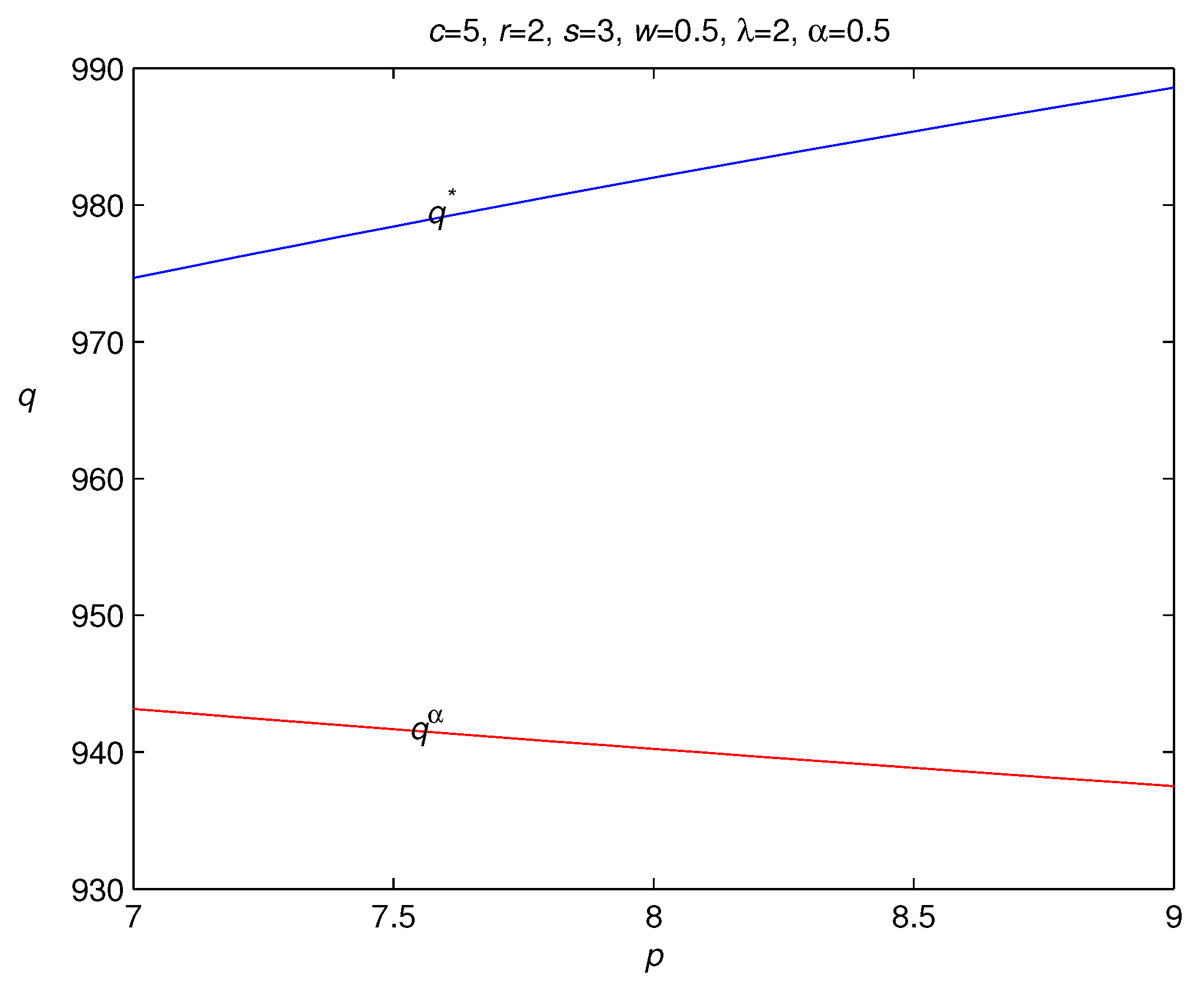
3.1. Optimal Order Quantity to Maximize Expected Utility

Since the realized market demand cannot be observed when the order quantity is decided, the realized utility from the given order quantity cannot be computed either. As a conventional method, we first study the optimal order quantity for the loss-averse newsvendor to maximize expected utility.

Theorem 1.

For the newsvendor model with backordering, the optimal order quantity for a loss-averse newsvendor to maximize expected utility is given as

$$q^{*}=F^{-1}\left[{\displaystyle \frac{(1-w)(p-c+\lambda s)}{(1-w)(p-c+\lambda s)+\lambda (c-r)}}\right].$$

Proof. 

For a given order quantity q and the realized market demand D, it follows from Equation (3) that

$$\begin{array}{c}\hfill U\left(q\right)=P\left(q\right)-\lambda L\left(q\right)=(p-c)min\{q,D\}+(p-c)w{(D-q)}^{+}\\ \hfill -\lambda [(c-r){(q-D)}^{+}+(1-w)s{(D-q)}^{+}].\end{array}$$

It follows from $min\{q,D\}=q-{(q-D)}^{+}$ and ${(D-q)}^{+}=D-q+{(q-D)}^{+}$ that

$$\begin{array}{c}\hfill U\left(q\right)=(1-w)(p-c+\lambda s)q+\left(w\right(p-c)-\lambda s(1-w\left)\right)D\\ \hfill -[(1-w)(p-c+\lambda s)+\lambda (c-r)]{(q-D)}^{+}.\end{array}$$

(5)

It follows from Equation (5) that the expected utility $E\left[U\right(q\left)\right]$ can be given as

$$\begin{array}{c}\hfill E\left[U\right(q\left)\right]=(1-w)(p-c+\lambda s)q+\left(w\right(p-c)-\lambda s(1-w\left)\right)E\left(\xi \right)\\ \hfill -[(1-w)(p-c+\lambda s)+\lambda (c-r)]{\int }_0^q(q-t)dF\left(t\right).\end{array}$$

(6)

Therefore, the first derivative of $E\left[U\right(q\left)\right]$ with respect to q is given as

$${\displaystyle \frac{\partial E\left[U\right(q\left)\right]}{\partial q}}=(1-w)(p-c+\lambda s)-[(1-w)(p-c+\lambda s)+\lambda (c-r)]F\left(q\right).$$

(7)

It follows form Equation (7) that the second derivative of $E\left[U\right(q\left)\right]$ with respect to q is given as

$${\displaystyle \frac{{\partial }^{2}E\left[U\left(q\right)\right]}{\partial q^2}}=-[(1-w)(p-c+\lambda s)+\lambda (c-r)]f\left(q\right)<0,$$

which implies that $E\left[U\right(q\left)\right]$ is concave in q and $E\left[U\right(q\left)\right]$ can attain the maximum value. Therefore, it follows from Equation (7) and the first-order condition that the optimal order quantity $q^{*}$ to maximize the expected utility $E\left[U\right(q\left)\right]$ satisfies

$$(1-w)(p-c+\lambda s)-[(1-w)(p-c+\lambda s)+\lambda (c-r)]F\left(q^{*}\right)=0,$$

which implies

$$q^{*}=F^{-1}\left[{\displaystyle \frac{(1-w)(p-c+\lambda s)}{(1-w)(p-c+\lambda s)+\lambda (c-r)}}\right].$$

This completes the proof.  □

In Theorem 1, $q^{*}$ is the optimal order quantity of q to maximize the expected utility of $E\left[U\right(q\left)\right]$. This result gives the optimal order quantity for a loss-averse newsvendor to maximize expected utility. When $\lambda =1$ and $w=0$, it means the loss-averse newsvendor turns to be loss-neutral and there are no backorders. It follows with $\lambda =1$ and $w=0$ in $q^{*}$ that

$$q^1=q^{*}{|}_{w=0,\lambda =1}=F^{-1}\left[{\displaystyle \frac{p-c+s}{p-r+s}}\right],$$

where $q^1$ represents the optimal order quantity of the loss-neutral newsvendor with no backorders. It is the same as the result obtained by Xu et al. [26], Gotoh and Takano [27] and Xu and Li [28].

Moreover, when $w=0$ and $s=0$, it means there are no backorders and no shortage cost for the lost sales. It follows with $w=0$ and $s=0$ in $q^{*}$ that

$$q^2=q^{*}{|}_{w=0,s=0}=F^{-1}\left[{\displaystyle \frac{p-c}{p-c+\lambda (c-r)}}\right],$$

where $q^2$ represents the optimal order quantity of the loss-averse newsvendor with no backorders and no shortage cost. It can be found that some existing results are the special cases of the optimal order quantity $q^{*}$. To study the properties of the optimal order quantity $q^{*}$, we have the following results.

Corollary 1.

For the newsvendor model with backordering, the optimal order quantity $q^{*}$ for a loss-averse newsvendor to maximize expected utility satisfies that

(i) 

$q^{*}$ is increasing in the retail price p;

(ii) 

$q^{*}$ is increasing in the salvage price r;

(iii) 

$q^{*}$ is increasing in the shortage cost s; and

(iv) 

$q^{*}$ is decreasing in the wholesale price c.

Proof. 

The proof is similar to that of Corollary 1 in the work of Xu and Li [28].

The above results are the same as the existing results on the traditional newsvendor model with expected profit maximization objective. The increase in the retail price and the shortage cost will increase the loss from lost sales, therefore the loss-averse newsvendor should order more items in such a case. However, the increase in the wholesale price can increase the order cost, and the loss-averse newsvendor should order fewer items in such a case.  □

Corollary 2.

For the newsvendor model with a backorder case, the optimal order quantity $q^{*}$ for a loss-averse newsvendor to maximize expected utility is decreasing in the backorder rate w.

Proof. 

It follows from Theorem 1 that the optimal order quantity $q^{*}$ is given as

$$q^{*}=F^{-1}\left[{\displaystyle \frac{(1-w)(p-c+\lambda s)}{(1-w)(p-c+\lambda s)+\lambda (c-r)}}\right].$$

The first derivative of $q^{*}$ with respect to w is given as

$${\displaystyle \frac{\partial q^{*}}{\partial w}}=-{\displaystyle \frac{1}{f\left[F^{-1}\left({\displaystyle \frac{(1-w)(p-c+\lambda s)}{(1-w)(p-c+\lambda s)+\lambda (c-r)}}\right)\right]}}{\displaystyle \frac{\lambda (p-c+\lambda s)(c-r)}{{[(1-w)(p-c+\lambda s)+\lambda (c-r)]}^2}}\le 0,$$

which implies $q^{*}$ is decreasing in the backorder rate w. This completes the proof. □

The intuition for this result is clear: if the backorder rate increases, more excess demands can be backlogged, therefore the loss comes more from the over-ordering items and then the loss-averse newsvendor should order fewer items to avoid the loss from over-ordering. In other words, backordering encourages the newsvendor to select a smaller order quantity. The bigger the backordering rate is, the fewer items the newsvendor orders.

Corollary 3.

For the newsvendor model with a backorder case, the optimal order quantity $q^{*}$ for a loss-averse newsvendor to maximize expected utility is decreasing in the loss aversion coefficient λ.

Proof. 

The proof is similar to that of Corollary 2.

When the loss aversion coefficient increases, the newsvendor becomes more loss-averse. According to this result, the loss-averse newsvendor who becomes more loss-averse should order fewer items. It is similar to the result presented by Schweitzer and Cachon [16]. Therefore, the loss aversion induces the newsvendor to order fewer items. The more loss-averse the newsvendor takes, the fewer items the newsvendor orders.  □

Corollaries 2 and 3 show that both backordering and loss aversion lead to a smaller order quantity. Therefore, the optimal order quantity $q^{*}$ is smaller than the optimal order quantities $q^1$ and $q^2$ obtained by Xu et al. [26], Gotoh and Takano [27] and Xu and Li [28]. This provides some interesting management insights for the loss-averse retailer in practice. For example, if more percentage of excess demands of the unsatisfied customers can be backlogged, the newsvendor should order fewer items to avoid the loss from over-ordering. Moreover, if the newsvendor becomes more loss-averse, he/she should order fewer items as well.

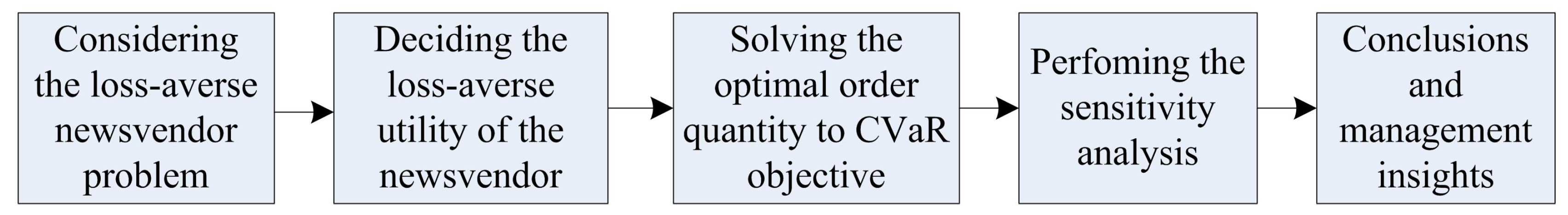
3.2. Risk Hedging in Loss-Averse Newsvendor Model with Backordering

In the above subsection, we derive the optimal order quantity for a loss-averse newsvendor to maximize expected utility. However, the expected utility maximization order quantity is not sufficient for the newsvendor to decide the optimal order decision in reality. In recent years, some unpredictable disasters have disrupted the supply chain operations repeatedly and the retailers in reality become more sensitive to loss. In 2011, Sony reported a loss of 1.99 billion dollars in its first quarter for supply chain disruptions caused by the earthquake in Japan in March 2011 https://www.supplychaindigital.com/procurement/sonys-supply-chain-hit-hard-japan-disaster. Toyota also announced a loss of 1.2 billion dollars in product revenue because of parts shortages resulting from this catastrophic earthquake-induced tsunami https://www.ebnonline.com/. Thus, many researchers have paid attention to risk hedging in the newsvendor model. For example, many researchers introduced the CVaR measure to cope with risk management in the newsvendor model (see [26,27,28,29,30,31,32,33,34,35,36,37]). However, to the best of our knowledge, the existing studies addressing risk management in the loss-averse newsvendor model do not consider the backorder case, while backlogging the excess demands in a stock-out situation becomes more and more common in reality. On the other hand, although backordering offers an effective mechanism to save the lost sales for a newsvendor, there are certain costs from backordering should be considered in the optimal decision process. When the backordering cost is very high, the cost from backlogging the excess demands will be very large. Therefore, it can also be a risky strategy if a newsvendor heavily relies on backordering to save the profit from the lost sales. In view of these issues, to hedge against potential risks in the loss-averse newsvendor model with backordering, we incorporate the CVaR measure into the decision framework of the loss-averse newsvendor model with a backorder case.

For the loss-averse newsvendor’s utility $U\left(q\right)$, we can define VaR about $U\left(q\right)$ for the loss-averse newsvendor as follows

$$Va{R}_{\alpha }\left[U\left(q\right)\right]=sup\{y\in R|Pr\{U\left(q\right)\ge y\}\ge \alpha \},$$

(8)

where $Pr\left\{U\right(q)\ge y\}$ denotes the probability of $U\left(q\right)$ exceeding value y. $Va{R}_{\alpha }\left[U\left(q\right)\right]$ represents the maximum profit the loss-averse newsvendor can obtain under the confidence level $\alpha$. Taking $Va{R}_{\alpha }\left[U\left(q\right)\right]$ as the targeted utility, the CVaR about utility $U\left(q\right)$ for a loss-averse newsvendor can be given as

$$CVa{R}_{\alpha }\left[U\left(q\right)\right]=E\left[U\left(q\right)\right|U\left(q\right)\le Va{R}_{\alpha }\left[U\left(q\right)\right]].$$

It represents the expected value of the utility which is below the target level $Va{R}_{\alpha }\left[U\left(q\right)\right]$. Then, we have the following result about the optimal order quantity to maximize the CVaR objective.

Theorem 2.

For the newsvendor model with a backorder case, the optimal order quantity for a loss-averse newsvendor to maximize CVaR about utility is given by

$$q^{\alpha }=\left\{\begin{array}{cc}M\hfill & s\le {\displaystyle \frac{w(p-c)}{\lambda (1-w)}},\hfill \\ {\displaystyle \frac{(p-c+\lambda (c-r\left)\right)M+\left(\lambda s\right(1-w)-w(p-c\left)\right)N}{(1-w)(p-c+\lambda s)+\lambda (c-r)}}\hfill & s>{\displaystyle \frac{w(p-c)}{\lambda (1-w)}},\hfill \end{array}\right.$$

where

$$M=F^{-1}\left[{\displaystyle \frac{(1-\alpha )(1-w)(p-c+\lambda s)}{(1-w)(p-c+\lambda s)+\lambda (c-r)}}\right],N=F^{-1}\left[{\displaystyle \frac{(1-\alpha )(1-w)(p-c+\lambda s)}{(1-w)(p-c+\lambda s)+\lambda (c-r)}}+\alpha \right].$$

Proof. 

See the Appendix A.  □

In Theorem 2, $q^{\alpha }$ represents the optimal order quantity for a loss-averse newsvendor to maximize the CVaR about utility. It is checked that, when $\alpha =0$, the risk-averse newsvendor becomes risk-neutral, and $q^{\alpha }$ is reduced to $q^{*}$ in Theorem 1. When $w=0$ and $\lambda =1$, the newsvendor becomes loss-neutral and there are no backorders; then, it follows with $w=0$ and $\lambda =1$ in $q^{\alpha }$ that

$$q^3=q^{\alpha }{|}_{w=0,\lambda =1}={\displaystyle \frac{(p-r)F^{-1}\left[{\displaystyle \frac{(1-\alpha )(p-c+s)}{(p-r+s)}}\right]+s{F}^{-1}[{\displaystyle \frac{(1-\alpha )(p-c+s)}{(p-r+s)}}+\alpha ]}{p-r+s}},$$

which is the same as the result presented by Gotoh and Takano [27] and Xu and Li [28].

Similar to Corollaries 1–3, we have the following results to show the properties of the optimal order quantity $q^{\alpha }$.

Corollary 4.

For the newsvendor model with backordering, the optimal order quantity $q^{\alpha }$ satisfies that

(i) 

$q^{\alpha }$ is increasing in the salvage price r; and

(ii) 

$q^{\alpha }$ is increasing in the shortage cost s.

Proof. 

First, it follows from Theorem 2 that

$$q^{\alpha }=\left\{\begin{array}{cc}M\hfill & s\le {\displaystyle \frac{w(p-c)}{\lambda (1-w)}},\hfill \\ {\displaystyle \frac{(p-c+\lambda (c-r\left)\right)M+\left(\lambda s\right(1-w)-w(p-c\left)\right)N}{(1-w)(p-c+\lambda s)+\lambda (c-r)}}\hfill & s>{\displaystyle \frac{w(p-c)}{\lambda (1-w)}}.\hfill \end{array}\right.$$

When $s\le {\displaystyle \frac{w(p-c)}{\lambda (1-w)}}$, we have

$$q^{\alpha }=M=F^{-1}\left[{\displaystyle \frac{(1-\alpha )(1-w)(p-c+\lambda s)}{(1-w)(p-c+\lambda s)+\lambda (c-r)}}\right].$$

Then, the first derivative of $q^{\alpha }$ with respect to r is given as

$${\displaystyle \frac{\partial q^{\alpha }}{\partial r}}={\displaystyle \frac{1}{f\left(M\right)}}{\displaystyle \frac{\lambda (1-\alpha )(1-w)(p-c+\lambda s)}{{[(1-w)(p-c+\lambda s)+\lambda (c-r)]}^2}}\ge 0.$$

(9)

Moreover, we have

$$F^{-1}\left[{\displaystyle \frac{(1-\alpha )(1-w)(p-c+\lambda s)}{(1-w)(p-c+\lambda s)+\lambda (c-r)}}\right]{|}_{s={\displaystyle \frac{w(p-c)}{\lambda (1-w)}}}=F^{-1}\left[{\displaystyle \frac{(1-\alpha )(p-c)}{p-c+\lambda (c-r)}}\right].$$

(10)

Otherwise, when $s>{\displaystyle \frac{w(p-c)}{\lambda (1-w)}}$, we have

$$q^{\alpha }={\displaystyle \frac{(p-c+\lambda (c-r\left)\right)M+\left(\lambda s\right(1-w)-w(p-c\left)\right)N}{(1-w)(p-c+\lambda s)+\lambda (c-r)}}.$$

The first derivative of $q^{\alpha }$ with respect to r is given as

$${\displaystyle \frac{\partial q^{\alpha }}{\partial r}}={\displaystyle \frac{\lambda (1-\alpha )(1-w)(p-c+\lambda s)}{{[(1-w)(p-c+\lambda s)+\lambda (c-r)]}^3}}[{\displaystyle \frac{p-c+\lambda (c-r)}{f\left(M\right)}}$$

$$+{\displaystyle \frac{\lambda s(1-w)-w(p-c)}{f\left(N\right)}}]+{\displaystyle \frac{\lambda \left(\lambda s\right(1-w)-w(p-c\left)\right)(N-M)}{{[(1-w)(p-c+\lambda s)+\lambda (c-r)]}^2}}\ge 0.$$

(11)

Moreover, it satisfies

$${\displaystyle \frac{(p-c+\lambda (c-r\left)\right)M+\left(\lambda s\right(1-w)-w(p-c\left)\right)N}{(1-w)(p-c+\lambda s)+\lambda (c-r)}}{|}_{s={\displaystyle \frac{w(p-c)}{\lambda (1-w)}}}=F^{-1}\left[{\displaystyle \frac{(1-\alpha )(p-c)}{p-c+\lambda (c-r)}}\right].$$

It follows from Equations (9)–(12) that ${\displaystyle \frac{\partial q^{\alpha }}{\partial r}}\ge 0$, which implies that $q^{\alpha }$ is increasing in the salvage price r. Similarly, we can prove that the optimal order quantity $q^{\alpha }$ is increasing in the shortage cost s. This completes the proof.  □

These results and explanations are the same as those in Corollary 1. However, we have the following results about the monotonicity of the optimal order quantity $q^{\alpha }$ regarding to the retail price and the wholesale price, which are different from the results in Section 3.1.

Remark 1.

It is pointed out that the optimal order quantity $q^{\alpha }$ might be increasing or decreasing in the retail price p. It follows from Theorem 2 that, when $s>{\displaystyle \frac{w(p-c)}{\lambda (1-w)}}$, we have

$$q^{\alpha }={\displaystyle \frac{(p-c+\lambda (c-r\left)\right)M+\left(\lambda s\right(1-w)-w(p-c\left)\right)N}{(1-w)(p-c+\lambda s)+\lambda (c-r)}}.$$

Therefore, the first derivative of $q^{\alpha }$ with respect to p is given as

$$\begin{array}{c}{\displaystyle \frac{\partial q^{\alpha }}{\partial p}}={\displaystyle \frac{\lambda (1-\alpha )(1-w)(c-r)}{{[(1-w)(p-c+\lambda s)+\lambda (c-r)]}^3}}\left[{\displaystyle \frac{p-c+\lambda (c-r)}{f\left(M\right)}}+{\displaystyle \frac{\lambda s(1-w)-w(p-c)}{f\left(N\right)}}\right]\\ -{\displaystyle \frac{\lambda \left[s\right(1-w)+w(c-r\left)\right](N-M)}{{[(1-w)(p-c+\lambda s)+\lambda (c-r)]}^2}}.\end{array}$$

(12)

If ${\displaystyle \frac{\partial q^{\alpha }}{\partial p}}>0$, the optimal order quantity $q^{\alpha }$ is increasing in the retail price p. Otherwise, ${\displaystyle \frac{\partial q^{\alpha }}{\partial p}}<0$ and the optimal order quantity $q^{\alpha }$ is decreasing in the retail price p. Moreover, it is also noted that the optimal order quantity $q^{\alpha }$ may be increasing, or decreasing in the wholesale price c. Similar to the above analysis, when $s>{\displaystyle \frac{w(p-c)}{\lambda (1-w)}}$, we can obtain the first derivative of $q^{\alpha }$ with respect to c as

$$\begin{array}{c}{\displaystyle \frac{\partial q^{\alpha }}{\partial c}}=-{\displaystyle \frac{\lambda (1-\alpha )(1-w)(p-r+\lambda s)}{{[(1-w)(p-c+\lambda s)+\lambda (c-r)]}^3}}\left[{\displaystyle \frac{p-c+\lambda (c-r)}{f\left(M\right)}}+{\displaystyle \frac{\lambda s(1-w)-w(p-c)}{f\left(N\right)}}\right]\\ +{\displaystyle \frac{\lambda \left[w\right(p-r)-(\lambda -1\left)\right(1-w\left)s\right](N-M)}{{[(1-w)(p-c+\lambda s)+\lambda (c-r)]}^2}}.\end{array}$$

If ${\displaystyle \frac{\partial q^{\alpha }}{\partial c}}>0$, the optimal order quantity $q^{\alpha }$ is increasing in the wholesale price c. Otherwise, ${\displaystyle \frac{\partial q^{\alpha }}{\partial c}}<0$ and the optimal order quantity $q^{\alpha }$ is decreasing in the wholesale price c. The above results show that the change directions of the optimal order quantity with regard to the retail price and the wholesale price are indefinite. These results are different from the previous study on the newsvendor model, where the optimal order quantity is definitely increasing in the retail price and decreasing in the wholesale price. We have the following management insights from these results. The increase in the retail price may lead to the decrease in the market demand, and it is better for the loss-averse newsvendor to order fewer items to avoid the risks from over-ordering. However, the previous study on the newsvendor model always results in the conclusion that a newsvendor should order more items when the retail price increases (Gotoh and Takano [27]; Xu and Li [28]; Chen et al. [29]), which contradicts this common fact. Therefore, our result presents a new ordering policy that is consistent with this common fact, and provides theoretical evidence to explain it for the loss-averse newsvendor. That is, a bigger retail price leads to a smaller market demand, and the loss-averse newsvendor should order fewer items to reduce the over-ordering loss when the retail prices increases. To illustrate this result, we have the following example.

Example 1.

Consider the newsvendor model with a backorder case. Suppose the market demand ξ follows the normal distribution $N(1000,{100}^2)$. Let $c=5$, $r=2$, $s=3$, $w=0.5$, $\lambda =2$ and $\alpha =0.5$. We compute the newsvendor’s optimal order quantities $q^{*}$ and $q^{\alpha }$ with different retail price p in Figure 2. Figure 2 shows that the optimal order quantity $q^{*}$ is increasing in the retail price, while the optimal order quantity $q^{\alpha }$ is decreasing in the retail price. Let $p=8$, $r=2$, $s=3$, $w=0.5$, $\lambda =2$ and $\alpha =0.5$; we compute the newsvendor’s optimal order quantities $q^{*}$ and $q^{\alpha }$ with different wholesale price c in Figure 3. Figure 3 shows that the optimal order quantity $q^{*}$ is decreasing in the wholesale price, while the optimal order quantity $q^{\alpha }$ is increasing in the wholesale price. These numerical results verify the results in Remark 1.

Corollary 5.

For the newsvendor model with a backorder case, the optimal order quantity $q^{\alpha }$ is decreasing in the backorder rate w.

Proof. 

The proof is similar to that of Corollary 4.

This result is similar to that in Corollary 2, where the newsvendor’s optimal order quantity to maximize expected utility is decreasing in the backorder rate. In other words, the newsvendor should order fewer items to hedge against potential risks when more percentage of excess demands in a stockout situation can be backlogged.  □

Corollary 6.

For the newsvendor model with a backorder case, the optimal order quantity $q^{\alpha }$ may be increasing or decreasing in the loss aversion coefficient λ.

Proof. 

The proof is similar to that of Corollary 4.

It is found that this result is different from that in Corollary 3, where the newsvendor’s optimal order quantity to maximize expected utility is decreasing in the loss aversion coefficient. Besides, this result is also different from that in Xu et al. [21], where the newsvendor’s optimal order quantity to maximize CVaR about utility without shortage cost is decreasing in the loss aversion coefficient. Indeed, if shortage cost is not considered, the loss comes only from the possible excess orders, therefore the newsvendor should order fewer items when he/she becomes more loss-averse. However, if the shortage cost is considered, the loss comes from the excess orders or the lost sales. If the loss from excess orders is bigger than that from lost sales, the newsvendor should order fewer items when he becomes more loss-averse. Otherwise, he/she should order more items. Therefore, the loss-averse should weigh the loss from over-ordering against that from lost sales and then choose the optimal order quantity to minimize the total loss. In the following, we give an example to illustrate this result.  □

Example 2.

Consider the newsvendor model with a backorder case. Suppose the market demand ξ follows the normal distribution $N(1000,{100}^2)$. It is assumed that the parameters are given as $p=8$, $c=5$, $r=4$, $s=6$, $w=0.4$ and $\alpha =0.5$. We compute the newsvendor’s optimal order quantities $q^{*}$ and $q^{\alpha }$ with different loss aversion coefficient in Figure 4. Figure 4 shows that the optimal order quantity $q^{*}$ is decreasing in the loss aversion coefficient, while the optimal order quantity $q^{\alpha }$ is increasing in the loss aversion coefficient. It is also found that when the loss aversion coefficient is small, the optimal order quantity $q^{*}$ is bigger than $q^{\alpha }$. However, when the loss aversion coefficient is sufficiently large, the optimal order quantity $q^{*}$ is smaller than $q^{\alpha }$.

Corollary 7.

For the newsvendor model with a backorder case, the optimal order quantity $q^{\alpha }$ may be increasing or decreasing in the confidence level α.

Proof. 

The proof is similar to that of Corollary 4.

A bigger confidence level means that the newsvendor tends to be more risk-averse. This result shows that, if the loss-averse newsvendor becomes more risk-averse, the optimal order quantity $q^{\alpha }$ may be bigger or smaller than the expected utility maximization order quantity. As we all know, a newsvendor’s potential risk comes from the excess orders or the lost sales that can not be backlogged. If the potential risks from excess orders is bigger than that from the lost sales, the newsvendor should choose a smaller order quantity. Otherwise, the newsvendor should choose a bigger order quantity to hedge against the potential risks. Therefore, the newsvendor should weigh the risk from over-ordering against that from under-ordering and then choose the optimal order quantity to hedge against possible risks. In the following, we give an example to show this result.  □

Example 3.

Consider the newsvendor model with a backorder case. Suppose the market demand ξ follows the normal distribution $N(1000,{100}^2)$. Let $p=8$, $c=5$, $r=4$, $s=6$, $w=0.1$ and $\lambda =2$. We calculate the newsvendor’s optimal order quantities $q^{*}$ and $q^{\alpha }$ with different confidence level α in Figure 5. It shows that the optimal order quantity $q^{\alpha }$ is first decreasing and then increasing in the confidence level. Correspondingly, the optimal order quantity $q^{\alpha }$ is first smaller and then bigger than the optimal order quantity $q^{*}$. Since the loss from lost sales $(p-c+s=9)$ is bigger than that from the excess order ($c-r=1$) and the backorder rate is small ($w=0.1$), the potential risks comes more from the lost sales. Therefore, a bigger order quantity is suggested when the confidence level is big.

4. Discussion

In the above sections, we study the optimal order quantity for a loss-averse newsvendor to maximize the CVaR of utility. The properties of the optimal order quantities for the loss-averse newsvendor with backordering are also discussed. Especially, we perform the sensitivity analysis on the optimal order quantities with respect to different decision variables. We also give the relationships between the optimal order quantities and the optimal order quantities in the existing papers. The conclusions reveal that we obtain some interesting results that are different from the existing papers and some management insights can be suggested for the loss-averse retailer in practice.

Now, we first give a comparative summary about these variables and corresponding results obtained in this paper and other existing studies in

Table 1. Signs of partial derivative of the optimal order quantities.

	Optimal Order Quantity (OOQ) q	${\displaystyle \frac{\mathit{\partial }\mathit{q}}{\mathit{\partial }\mathit{p}}}$	${\displaystyle \frac{\mathit{\partial }\mathit{q}}{\mathit{\partial }\mathit{c}}}$	${\displaystyle \frac{\mathit{\partial }\mathit{q}}{\mathit{\partial }\mathit{r}}}$	${\displaystyle \frac{\mathit{\partial }\mathit{q}}{\mathit{\partial }\mathit{s}}}$	${\displaystyle \frac{\mathit{\partial }\mathit{q}}{\mathit{\partial }\mathit{\alpha }}}$	${\displaystyle \frac{\mathit{\partial }\mathit{q}}{\mathit{\partial }\mathit{\lambda }}}$	${\displaystyle \frac{\mathit{\partial }\mathit{q}}{\mathit{\partial }\mathit{w}}}$
	EPM order quantity in newsvendor model	+	−	+	+	n/a	n/a	n/a
	OOQ in Chen et al. [29]	+	−	+	n/a	−	n/a	n/a
	OOQ in Gotoh and Takano [27]	+	−	+	+	$+/-$	n/a	n/a
	OOQ in Schweitzer and Cachon [16]	+	−	+	n/a	n/a	−	n/a
	OOQ in Wang and Webster [17]	$+/-$	$+/-$	+	+	n/a	$+/-$	n/a
	$q^{*}$ in this paper	+	−	+	+	n/a	−	−
	$q^{\alpha }$ in this paper	$+/-$	$+/-$	+	+	$+/-$	$+/-$	−

. Table 1 describes the signs of the partial derivative of some optimal order quantities in the newsvendor model with respect to different decision variables. It is found that, when loss aversion is not considered, all the signs of the sensitivity to decision variables p, c, r and s remain the same as those of the EPM order quantity in the classical newsvendor model. However, when loss aversion and shortage cost are considered, the optimal order quantity may be decreasing in the retail price p and increasing in the wholesale price c, which is different from those results in the classical newsvendor model. In essence, since shortage cost is considered, the loss-averse newsvendor should consider both over-ordering loss and under-ordering loss in choosing the optimal order quantity. By Table 1, our study shows that the optimal order quantity for the loss-averse newsvendor to maximize the CVaR of utility can be decreasing in the retail price and increasing in the wholesale price, which is different from the previous newsvendor literature.

In Table 1, it is also observed that all signs of the sensitivity to r and s remain the same as those of the EPM order quantity in the classical newsvendor model, whereas the sensitivity to the confidence level $\alpha$ can differ from model to model as illustrated above. It can also be explained by over-ordering loss and under-ordering loss. For example, when the over-ordering loss is bigger than the under-ordering loss, the newsvendor should order fewer items as the confidence level $\alpha$ increases, otherwise, the newsvendor should order more items when he/she becomes more risk-averse. In particular, our study shows that, when s is sufficiently large and the loss from lost sales is bigger than the loss from over-ordering, the newsvendor should order more items when he/she becomes more loss-averse or risk-averse. These results aare illustrated in Example 3.

Table 1 also shows that the sign of the optimal order quantity with the sensitivity to $\lambda$ is not deterministic, especially when shortage cost is considered. In fact, when the shortage cost is included, the under-ordering loss becomes bigger with the increase of the shortage cost, therefore the sign of the optimal order quantity with the sensitivity to $\lambda$ may be changed in such a case. However, when shortage cost is not considered, the loss comes only from the possible lost sales, and the newsvendor should take a smaller order quantity when he/she becomes more loss-averse. The above analysis reveals that loss aversion and risk aversion may explain the decision bias in newsvendor model (Schweitzer and Cachon [16]). That is, the risk or loss preference induces the newsvendor to give a bigger or smaller order quantity than the EPM order quantity. This is consistent with the experimental results presented by Schweitzer and Cachon [16], i.e., subjects often order too few high-profit products and too many low-profit products. Table 1 also shows that the loss-averse newsvendor should order fewer items when the the backorder rate increases, which has never been studied in the existing literature. Our analysis shows that risk preference or loss preference can be alternative choices to explain the above experimental results of Schweitzer and Cachon [16].

The above results present some management insights for the loss-averse retailer in practice to hedge against potential risks. First, when backordering is considered, the loss-avers newsvendor should order fewer items as backordering can save all or part of the lost sales. The greater the percentage of lost sales that can be backlogged, the fewer items the retailer should order. Second, for a loss-averse retailer who becomes more risk-averse, he/she should first weigh the over-ordering risk against with the under-ordering risk and then choose the order quantity. That is, the retailer should select a smaller order quantity when the over-ordering risk is bigger than the under-ordering risk, and select a bigger order quantity when the over-ordering risk is smaller than the under-ordering risk. Third, when the salvage price and shortage penalty price increases, the loss-averse newsvendor should increase the order quantity to hedge against potential risks. Fourth, when the backorder rate increases, the loss-averse newsvendor should order fewer items to decrease the backorder cost. This study thus contributes to the risk management of the loss-averse newsvendor model and also lends insight into how backordering influences the optimal ordering policies of the loss-averse retailer in reality.

5. Conclusions

In this paper, we study the optimal ordering decisions of the loss-averse newsvendor model with a backorder case. To hedge against potential risks, we introduce the CVaR measure and obtain the optimal order quantity for a loss-averse newsvendor to maximize CVaR about utility. Our paper obtains some interesting results on the loss-averse newsvendor model with backordering. It is found that a newsvendor should order fewer items in a backordering setting to hedge against potential risks since backordering can save some lost sales. Moreover, it is shown that the optimal order quantity for a loss-averse newsvendor to maximize CVaR about utility may be decreasing in the retail price and increasing in the wholesale price, which is different from the results in the traditional newsvendor literature. Indeed, the previous study on the newsvendor model always suggests a bigger order quantity when the retail price increase. It is explained that a bigger retail price implies a bigger unit profit for each item for this result. However, it is a common fact that a bigger retail price usually comes with a smaller market demand. Therefore, when the retail price increases, the market demand decreases and the increase in the order quantity may lead to a bigger over-ordering risk. Moreover, since the excess demands can be all or partially backlogged and it is no need to order more items of product in a backorder setting, especially when the backorder rate is large. Similar arguments can be obtained on the change direction of the optimal order quantity with regard to the variation of the wholesale price. From this viewpoint, our result presents a more reasonable ordering policy for the loss-averse newsvendor in a backorder setting to hedge against potential risks and reduce possible losses. Further, we study the optimal order quantity for a loss-averse newsvendor to maximize the expected loss-averse utility, and it is found that the newsvendor should weigh the loss from over-ordering against that from lost sales and then choose the optimal order quantity. It is also found that this optimal order quantity may be increasing or decreasing in the confidence level in different cases. Therefore, the newsvendor needs to weigh the risk from over-ordering against that from under-ordering before deciding the optimal order quantity. Our paper thus provides some management insights for the risk management of the loss-averse newsvendor with backordering and lends insights into how backordering influences the optimal order decisions of the loss-averse newsvendor.

Some future studies are possible. To encourage the unsatisfied customers to accept the backorder invitation, some newsvendors provide price discount on retail price for the backlogged items [38,39,40]. Thus, a possible extension on this study would be introducing price discount on retail price into this research. Another possible extension is to consider a random backorder rate, which is more popular in practice. It is a more interesting but complicated case.

References

1. Gruen, T.; Corsten, D. Rising to the challenge of out-of-stocks. ECR J. 2002, 2, 45–58. [Google Scholar]
2. Montgomery, D.C.; Bazaraa, M.S.; Keswani, A.K. Inventory models with a mixture of backorders and lostsales. Naval Res. Logist. Q. 1973, 20, 255–263. [Google Scholar] [CrossRef]
3. Pando, V.; San, J.L.A.; García-Laguna, J.; Sicilia, J. A newsboy problem with an emergency order under a general backorder rate function. Omega 2013, 41, 1020–1028. [Google Scholar] [CrossRef]
4. San José, L.A.; Sicilia, J.; Garciá-Laguna, J. Analysis of an inventory system with exponential partial backordering. Int. J. Prod. Econ. 2006, 100, 76–86. [Google Scholar] [CrossRef]
5. Lodree, J.E.J. Advanced supply chain planning with mixture of backorders, lost sales, and lost contract. Eur. J. Oper. Res. 2007, 181, 168–183. [Google Scholar] [CrossRef]
6. Lodree, J.E.J.; Kim, Y.; Jang, W. Time and quantity dependent waiting costs in a newsvendor problem with backlogged shortages. Math. Comput. Model. 2008, 47, 60–71. [Google Scholar] [CrossRef]
7. Zhou, Y.; Wang, S. Manufacturer-buyer coordination for newsvendor-type-products with two ordering opportunities and partial backorders. Eur. J. Oper. Res. 2009, 198, 958–974. [Google Scholar] [CrossRef]
8. Chen, J.; Huang, S.; Hassin, R.; Zhang, N. Two backorder compensation mechanisms in inventory systems with impatient customers. Prod. Oper. Manag. 2015, 24, 1640–1655. [Google Scholar] [CrossRef]
9. Liu, S.D.; Song, M.; Tan, K.C.; Zhang, C.Y. Multi-class dynamic inventory rationing with stochastic demands and backordering. Eur. J. Oper. Res. 2015, 244, 153–163. [Google Scholar] [CrossRef]
10. Hsu, L.F.; Hsu, J.T. Economic production quantity (EPQ) models under an imperfect production process with shortages backordered. Int. J. Syst. Sci. 2016, 47, 852–867. [Google Scholar] [CrossRef]
11. Braglia, M.; Castellano, D.; Gallo, M. Approximate d close d-form minimum-cost solution to the (r,q) policy with complete backordering and further developments. Appl. Math. Model. 2016, 40, 8406–8423. [Google Scholar] [CrossRef]
12. Bao, L.N.; Liu, Z.Y.; Yu, Y.M.; Zhang, W. On the decomposition property for a dynamic inventory rationing problem with multiple demand classes and backorder. Eur. J. Oper. Res. 2018, 265, 99–106. [Google Scholar] [CrossRef]
13. Khouja, M. The single-period (news-vendor) problem: Literature review and suggestions for further research. Omega 1999, 27, 537–553. [Google Scholar] [CrossRef]
14. Qin, Y.; Wang, R.; Vakharia, A.J.; Chen, Y.; Michelle, M.H.S. The newsvendor problem: Review and directions for further research. Eur. J. Oper. Res. 2011, 213, 361–374. [Google Scholar] [CrossRef]
15. Kahneman, D.; Tversky, A. Prospect theory: An analysis of decision under risk. Econometrica 1979, 47, 263–291. [Google Scholar] [CrossRef]
16. Schweitzer, M.E.; Cachon, G.P. Decision bias in the newsvendor problem with a known demand distribution: Experimental evidence. Manag. Sci. 2000, 46, 404–420. [Google Scholar] [CrossRef]
17. Wang, C.X.; Webster, S. The loss-averse newsvendor problem. Omega 2009, 37, 93–105. [Google Scholar] [CrossRef]
18. Zhang, B.F.; Wu, D.S.; Liang, L.; Olson, D.L. Supply chain loss averse newsboy model with capital constraint. IEEE Trans. Syst. Man Cybern. Syst. 2016, 46, 646–658. [Google Scholar] [CrossRef]
19. He, Y.; Xu, Q.Y.; Xu, B.; Wu, P.K. Supply chain coordination in quality improvement with reference effects. J. Oper. Res. Soc. 2016, 67, 1158–1168. [Google Scholar] [CrossRef]
20. Vipin, B.; Amit, R.K. Loss aversion and rationality in the newsvendor problem under recourse option. Eur. J. Oper. Res. 2017, 261, 563–571. [Google Scholar] [CrossRef]
21. Xu, X.; Chan, C.K.; Langevin, A. Coping with risk management and fill rate in the loss-averse newsvendor model. Int. J. Prod. Econ. 2018, 195, 296–310. [Google Scholar] [CrossRef]
22. Artzner, P.; Delbaen, F.; Eber, J.M.; Heath, D. Coherent measures of Risk. Math. Finance 1999, 9, 203–228. [Google Scholar] [CrossRef]
23. Mauser, H.; Rosen, D. Beyond VaR: From measuring risk to managing risk. ALGO Res. Q. 1999, 1, 5–20. [Google Scholar]
24. Rockafellar, R.T.; Uryasev, S. Optimization of Conditional Value-at-Risk. J. Risk 2000, 2, 21–41. [Google Scholar] [CrossRef]
25. Rockafellar, R.T.; Uryasev, S. Conditional value-at-risk for general loss distributions. J. Bank. Finance 2002, 26, 1443–1471. [Google Scholar] [CrossRef] [Green Version]
26. Xu, M.; Yu, G.; Zhang, H. CVaR in a newsvendor model with lost sale penalty cost. Syst. Eng. Theory Pract. 2006, 26, 1–8. (In Chinese) [Google Scholar]
27. Gotoh, J.; Takano, Y. Newsvendor solutions via conditional value-at-risk minimization. Eur. J. Oper. Res. 2007, 179, 80–96. [Google Scholar] [CrossRef]
28. Xu, M.; Li, J. Optimal decisions when balancing expected profit and conditional value-at-risk in newsvendor models. J. Syst. Sci. Complex. 2010, 23, 1054–1070. [Google Scholar] [CrossRef]
29. Chen, X.; Sim, M.; Simichi-levi, D.; Sun, P. Risk Aversion in Inventory Management; MIT: Cambridge, MA, USA, 2003. [Google Scholar]
30. Chen, Y.; Xu, M.; Zhang, Z.G. A risk-averse newsvendor model under the CVaR criterion. Oper. Res. 2009, 57, 1040–1044. [Google Scholar] [CrossRef]
31. Li, Y.; Lin, Q.; Ye, F. Pricing and promised delivery lead time decisions with a risk-averse agent. Int. J. Prod. Res. 2014, 52, 3518–3537. [Google Scholar] [CrossRef]
32. Alonso-Ayuso, A.; Escudero, L.F.; Guignard, M.; Weintraub, A. Risk management for forestry planning under uncertainty in demand and prices. Eur. J. Oper. Res. 2018, 267, 1051–1074. [Google Scholar] [CrossRef]
33. Xie, Y.; Wang, H.W.; Lu, H. Coordination of supply chains with a retailer under the mean-CVaR criterion. IEEE Trans. Syst. Man Cybern. Syst. 2018, 48, 1039–1053. [Google Scholar] [CrossRef]
34. Xu, X.; Meng, Z.; Shen, R. A tri-level programming model based on Conditional Value-at-Risk for three-stage supply chain management. Comput. Ind. Eng. 2013, 66, 470–475. [Google Scholar] [CrossRef]
35. Xu, X.; Meng, Z.; Shen, R.; Jiang, M.; Ji, P. Optimal decisions for the loss-averse newsvendor problem under CVaR. Int. J. Prod. Econ. 2015, 164, 146–159. [Google Scholar]
36. Xu, X.; Meng, Z.; Ji, P.; Dang, C.; Wang, H. On the newsvendor model with conditional Value-at-Risk of opportunity loss. Int. J. Prod. Res. 2016, 54, 2449–2458. [Google Scholar] [CrossRef]
37. Xu, X.; Wang, H.; Dang, C.; Ji, P. The loss-averse newsvendor model with backordering. Int. J. Prod. Econ. 2017, 188, 1–10. [Google Scholar] [CrossRef]
38. Johansen, S.G.; Thorstenson, A. Emergency orders in the periodic-review inventory system with fixed ordering costs and compound Poisson demand. Int. J. Prod. Econ. 2014, 157, 147–157. [Google Scholar] [CrossRef]
39. Ruan, J.; Wang, Y.; Chan, F.T.S.; Hu, X.; Zhao, M.; Zhu, F.; Shi, B.; Shi, Y.; Lin, F. A life-cycle framework of green IoT based agriculture and its finance, operation and management issues. IEEE Commun. Mag. 2019, 57, 90–96. [Google Scholar] [CrossRef]
40. Xu, X.; Chan, F.T.S.; Chan, C.K. Optimal option purchase decision of a loss-averse retailer under emergent replenishment. Int. J. Prod. Res. 2019. [Google Scholar] [CrossRef]
Figure 1. The flowchart of this research.
Mathematics 07 00429 g001
Figure 2. Optimal order quantities q * and q α with different retail price p.
Mathematics 07 00429 g002
Figure 3. Optimal order quantities q * and q α with different wholesale price c.
Mathematics 07 00429 g003
Figure 4. Optimal order quantities q * and q α with different loss aversion coefficient λ .
Mathematics 07 00429 g004
Figure 5. Optimal order quantities q * and q α with different confidence level α .
Mathematics 07 00429 g005