Data-Driven Iron and Steel Inventory Control Policies


1
Department of Business Administration, Chung Yuan Christian University, 200 Chung Pei Road, Chung Li District, Taoyuan City 32023, Taiwan
2
Department of Information Technology, Walsin Lihwa Corporation, 25F, No.1, Songzhi Rd., Taipei 11047, Taiwan
*
Author to whom correspondence should be addressed.
Mathematics 2019, 7(8), 718; https://doi.org/10.3390/math7080718
Submission received: 12 July 2019
/
Revised: 3 August 2019
/
Accepted: 5 August 2019
/
Published: 7 August 2019
Abstract
:In this study, we investigated the optimal material inventory policy with regard to the iron and steel industry’s effort to reduce massive overstocking issues in the face of increased corporate competitiveness. We gathered actual data, including sales and inventory numbers, from a steel and iron company over a period of 216 weeks between January 2010 and February 2014. We then utilized the Markov decision process (MDP) to analyze this data for inventory problems, such as relevant reorder points and reorder quantity issues as they relate to lead time, stock on hand and the limitations of having stock in-transit. The purpose of the study was to determine the most effective method for minimizing costs by using the optimal inventory policy to calculate and verify the effectiveness of the results. The final 52 weeks of data were put aside, while the initial 164 weeks were used to create an inbound material receipt system to ultimately establish a yearly (52-week) policy based on the inventory and sales data for weeks 113–164. Finally, we verified the effectiveness of the policy using the data from the final 52 weeks. The results showed that our proposed categorization method was effective for reducing the quantity of inventory while still meeting quarterly demands.
1. Introduction
Product diversification is a prominent aspect of today’s business environment, which makes it more of a challenge to maintain an adequate supply of materials on hand to satisfy downstream customers. The costs of storing these materials include management, holding, and land costs as well as damage liability and risk, which decrease the profits of a company [1]. However, insufficient product supply can lead to delays or extended delivery schedules and loss of many customers. When developing a market, effective inventory management strategies are essential to maximize profits.
The most pressing issue on every manager’s mind is determining exactly how much stock to order and when (also known as reorder point and reorder quantity). Although the more traditional economic order quantity (EOQ) model [2] and the material requirement planning (MRP) method [3] can be of help when facing these issues, the (s,S) policy [4,5,6,7,8,9,10] and the Markov decision process (MDP) [11,12] have also been touted by many scholars as more modern and effective techniques for solving inventory management issues. These methods are all based on set parameters for the purpose of finding the optimal policy that minimizes costs and maximizes profits. The problem is that many scholars have based their analyses on mock data rather than actual data from real businesses [13,14,15,16,17], resulting in a great disparity between theoretical results and practical applications of these methods [18].
The issues of inventory management must be dealt with over a long period of time; [11] however, the EOQ, MRP, and (s,S) policies for simplified optimal solutions are only able to meet short-term goals when faced with unpredictable levels of demand. When we look at the larger picture, we realize that only the MDP is able to adapt to changing circumstances and offer new policy recommendations to satisfy quarterly demands [19]. This strategy has also been widely used to analyze complicated, long-term strategy issues in many diverse areas, including queuing theory [20], inventory [12], maintenance [21], finance [22], disease treatment [23], and water reservoir maintenance [24].
An analysis of Taiwan Industry Economics Services on April, 2014 [25]) makes it clear that the overstocking of materials during a period of falling steel prices eroded the company’s profits. Global trends over the last two years have made it essential for the iron and steel industry to solve inventory management issues. Isotupa [26] studied the critical elements of lead time and safety stock via probability distribution within set parameters by feeding data into the ARENA program and using probability distribution to interpret it. The surprising results revealed that regardless of the data used, the probability distribution (including the common index distributions) and the use of actual company data within set parameters highlights many modern inventory management issues.
We decided to further test this method by utilizing it to develop an optimal inventory policy. We obtained permission from a steel and iron manufacturer to gather inventory data including dates, initial inventory, sales figures, and ending inventory over a period of 216 weeks from January 2010 to February 2014. Numerous production processes and longer manufacturing times in the steel industry mean that orders are usually received up to six months in advance. This makes the sales volume more predictable and relatively stable, although actual delivery times might be affected. After utilizing the MDP to establish an optimal inventory policy, we then compared the results to those obtained via EOQ, MRP, and (s,S) policies.
In Section 2, we introduce the MDP model and describe all the states, actions, and transition probabilities involved. In Section 3, we discuss the company case study and outcome of each action. In Section 4, we present the results of our analysis of the case study. Our conclusions and suggestions for future research are presented in Section 5.
2. Literature Review
2.1. Definition and Function of Inventory
In a complete production process, the inventory policy directly affects the profitability of a company. Upon arrival at a manufacturing plant, raw materials are processed at one or many work stations, sent to the warehouse for storage, and later used to manufacture the product. The efficiency of this process depends not only on the quantity of raw materials in inventory, but on the timing of their arrival so as to avoid having too much or too little material in inventory at any given time. Too little inventory in stock leads to sales losses and declining customer satisfaction, which ultimately leads to shortage costs. Too much inventory in stock brings about unnecessary holding costs. As such, inventory managers must guarantee low-inventory standards and satisfy customers in the face of uncertain demand.
Render and Heizer [27] argue that the objective of inventory management is to achieve a balance between inventory costs and customer service. In addition, a suitable amount of inventory not only provides a company with greater operating flexibility but it also reduces demand fluctuations for the company’s product, offers customers an adequate range of product options, and reduces transportation costs for products via bulk purchases. Offering discounts for buying in bulk can counter inflation and adjust upstream prices.
2.2. Major Factors Affecting Inventory
2.2.1. Lead Time
Although the value of lead time in many models is zero, [28] it is important for more highly competitive companies. Hoque [29] proposes that lead time is one of the major factors that affect inventory management because it encompasses time spent on reviewing orders, the ordering process, supplier lead time, transport time, and time spent receiving goods. Basically, lead time includes employee hours spent on all processes from the initial ordering of materials from the supplier to when the materials arrive at the warehouse. Too little lead time directly affects profits and makes buying the correct quantities for safety stock even more difficult.
Other related research on lead time includes a study by Rossi et al. [30] who utilized random lead times to analyze inventory management issues. In a related study, Sajadieh et al. [31] analyzed lead time via index distribution and found that it has a significant effect on company efficiency and profitability, the degree of which varies from industry to industry. Arikan et al. [32] argued that the economic environment affects lead time, which is vital, particularly in the iron and steel industry. After much consultation with various companies, we used actual data to analyze lead time, which we believe will be more effective for helping companies to reduce the uncertainties associated with both the external environment and internal factors.
2.2.2. Safety Stock
Generally, it is necessary to maintain a certain level of inventory to be able to effectively respond to changing demands during the production process and fill unexpected orders that may be placed during the lead time. This level of inventory is known as safety stock, which is generally calculated based on the fluctuations of stock levels, including in-transit stock, at the end of each quarter. This formula is normally safety stock = internal base safety stock + average demand * lead time.
2.2.3. Inventory Costs
The quantity of materials ordered directly affects the company’s profitability by significantly changing costs that include ordering materials from a supplier, internal setup costs, holding fees for materials that have not been used, and shortage costs for materials kept in insufficient quantities. The following definitions are from Render and Heizer [27].
- Ordering costs are associated with suppliers, forms, order and purchase processing, and record keeping.
- Setup costs involve the machinery and production processes. They are closely related to setup time.
- Holding costs are associated with inventory maintenance.
- Shortage costs include all potential profit sacrificed due to a loss of business opportunities and customers, which arise from a shortage of materials.
In our study, ordering, setup, and holding costs were all closely related to the quantities of iron and steel, and costs were calculated per kilogram of material. Since setup costs involve machinery, preparation for production processes are closely related to production quantity. The amount of scheduled production will also affect safe inventory levels. Thus, all analyses of cost considerations in this paper are in the form of “number of kilograms.” The company we studied avoided inventory shortages at all costs. The product categories analyzed in this paper are for mainstream products. If a product is in short supply, cost to the company in compensation can be huge and late deliveries can irreparably damage the reputation of the company. Hence, we set aside a great deal of money in our model to cover potential shortage costs. Therefore, shortage costs were defined as limitless and were included in the actual calculations at a value of +99,999,999 to eliminate the possibility of shortages from the analysis process, discussed in Section 4.
2.3. Methods of Inventory Control
Analysis of inventory management issues, which require many different methods of research, often focus on reorder points and quantities. The objective is always to determine the appropriate times and quantities to reorder so as to minimize total inventory-related costs. The most well-known theories, ABC analysis and the economic order quantity model (EOQ Model), are used to assist company managers with material requirement planning (MRP).
2.3.1. ABC Analysis
ABC analysis, also known as cycle counting, is an early simple method used in the field of inventory management. It only defines the classification method for products and does not specify the order quantity. Therefore, in this study, we used the MDP method for analysis. In the case of most large-scale products (A-type products), company executives must find the optimal policy for each period, a method that utilizes the concept of ABC analysis. Thus, it was not implemented for analyzing this value. This method, which is often used in materials management, involves dividing the inventory into various categories. Also known as optional inventory management, it offers an effective basis for categorization and significantly reduces warehousing costs [33]. Wild [34] defines the categories used in this method based on yearly revenue as follows:
- A: 10% of inventory items yield 66.6% of revenue.
- B: 20% of inventory items garner 23.3% of revenue.
- C: 70% of inventory items are worth 10.1% of the total revenue.
According to ABC analysis, a higher percentage of resource purchasing should be invested in Category A items from the supplier than on Category B and C items. In addition, Category A items should be subjected to stricter inventory controls than the other items, meaning that popularity of Category A items should be seen as more predictive of future demand. Therefore, it is essential to accurately record these items and subject them to continuous checks and inspections, known as cycle counting. The following shows the count frequencies for each category:
- Category A items are counted frequently (e.g., once a month).
- Category B items are counted slightly less often than those of Category A (e.g., once a quarter).
- Category C items are rarely counted (e.g., once every six months or less).
2.3.2. The Economic Order Quantity Model
The oldest quantity method of inventory management is Harris’ [2] economic order quantity (EOQ) model, which reduces inventory holding and order costs by minimizing the optimal order quantity. It is based on the following assumptions: (1) Order costs are constant, (2) annual product demand is both constant and known ahead of time, (3) no discounts are available for bulk purchases, and (4) there is no lead time. The optimal ordering quantity was calculated using the equation Q * = , where A represents ordering costs, D signifies demand, and h represents holding costs within a particular unit of time.
The traditional economic order quantity model is still relevant today as its concepts are simple and easy to implement, factors which have led to its widespread adoption. However, the four assumptions described above are not necessarily applicable to real-world situations, which intensifies the search for a more comprehensive and realistic method of analysis. Many scholars have proposed improvements to the model but none of the new approaches have been able to rise above these inherent limitations.
2.3.3. Material Requirement Planning
MRP, a type of business management software born primarily from the traditional order point system, is aimed at effective management of company production processes, including warehousing and manufacturing.
In this system, all materials, half-finished products, and equipment used in the production process are separated into bills of material (BOM) based on their structure and demand. The purpose of MRP is to implement demand-based ordering of materials.
2.3.4. (s,S) Policy
A large number of business owners and researchers currently use the (s,S) policy to manage their inventory. This policy requires managers to regularly check their current inventory and purchase an S-s quantity of material from suppliers whenever their inventory falls below s. Implementation of this method allows managers to determine reorder points (s) and order quantities (Q = S−s), allowing for effective control of inventory.
2.4. Markov Decision Process
2.4.1. Dynamic Programming Concepts
Although many companies have their own internal mechanisms for selecting order quantities, they will still occasionally have a sudden need for larger amounts or will face a sudden drop in demand. This makes using a single ordering model impractical. Instead, utilizing several different policies simultaneously can greatly reduce the inherent risks of relying on a single ordering model.
Dynamic programming concepts are, therefore, particularly important. This method involves breaking problems down into their smallest and simplest components and seeking resolutions for them first. The purpose of these techniques is to create policy solutions for single-chain production. The spirit of dynamic programming is based on the principle of optimality, proposed by Bellman [35], which states, “An optimal policy has the property that whatever the initial state and initial decisions are, the remaining decisions must constitute an optimal policy with regard to the state resulting from the first decision.”
Dynamic programming utilizes repetitive features to uncover an overall resolution for issues and resolve complicated, multi-level policy problems while maximizing (or minimizing) objective function forecasts to actively maximize total profits (or minimize total costs) with a single-chain policy known as the optimal technique. As inventory management problems are single-chain issues, in this study, we sought solutions using the dynamic programming model.
2.4.2. Markov Decision Process Elements
The Markov decision process, named for the Russian mathematician Andrey Markov, offers a mathematical analysis of circumstances that are partly random and partly determined by the policy-maker. This technique has been widely adopted and continues to be in demand to this day.
In addition, many scholars have used it for inventory management to determine optimal order points and quantities, to implement sensitivity analyses, to measure fluctuations of policy variables, and to determine final overall changes in profit. Its main purpose is to provide a value analysis using given probability distribution assumptions and to expand inventory control analysis results [36]. Four major elements are required to employ the MDP:
- State is a collection of all possible circumstances at each stage in the system.
- Transition probability matrix is defined by the current states and selected policies. This is completely separate from the variables of past states and past selected policies.
- Action is defined as a collection of all policies that form the options available to the decision-maker at each state. The system will happen the following two events when the decision-maker chooses any action in any state: (1) The decision-maker will receive the appropriate profits associated with that action, and (2) the system will exchange one of the states in the collection for the following states based on this action.
- Rewards are defined as evaluations of the performance of the Markov process based on the profits or costs related to a particular action.
3. Study Overview and Research Methods
3.1. Study Overview
The data used in this study came from a well-known Taiwanese iron and steel company that has been listed among Taiwan’s top 1000 manufacturers by Common Wealth Magazine. This particular company was established in July 1988 and sells mainly plastic mold steel, cold and hot work steel, as well as PM high speed and breathable steel. It supplies specialized materials for optics and medical components as well as electronic parts for the automotive industry, semiconductors, and all high-, medium-, and low-end product molds for automation. It must be noted that this company has a large client base all over the world.
This company was established during a period of rising steel prices and was able to minimize costs by purchasing large quantities of steel and holding them in stock, which gave it a significant competitive advantage. This technique slowly became the company’s main method of inventory management; however, the price of steel has continued to fall in recent years, making it cheaper to delay purchases and negating the need to stockpile in advance. Due to these falling prices, excess inventory now negatively affects the company profits in intangible ways in addition to the more concrete holding costs. Competition is fierce in the industry and a shortage of materials would immediately result in customers switching to another supplier, which obviously would negatively impact both the immediate profits and future business opportunities. Ordering policies cannot be changed without proper planning, as the company cannot risk an inventory shortage. For this reason, the development of an appropriate inventory policy has been a major hurdle for this company.
3.2. Data Properties and Model Establishment
3.2.1. Data Properties
There are many types of inventory and just as many inventory analysis tools that focus on various aspects of this complex business. Table 1 shows the average values and standard deviation for the ending inventory. The data period examined in this study was 216 weeks from January 2010 to February 2014. This paper stands for the minimum cost in 52 weeks, first retains the last 52 weeks of data, and the previous 164 weeks of data was used for inventory. We formulated the policy and validated it with the information from the 52-week period. The descriptive statistics of the data such as the average number and standard deviation were calculated based on data from the first 164 weeks, January 2010 to February 2013. As seen below, the properties of the data are represented by the coefficient of variation (Cv), which is a comparison of the standard deviation and average value, indicating unit risk. When comparing two or more groups of data with different averages, the standard deviation will provide an accurate description of the data [3]. To examine the inventory management, the coefficients of the highs and lows mainly fall at the edges of different types of data areas and are used to observe whether or not these trends can be applied to the optimal data policy [37]. Table 1 shows an analysis of the basic data. The average ending inventory was 47,531.64 kg, the standard deviation was 26,145.70 kg, and the coefficient of the variation was 0.55.
3.2.2. Actions, States, Transitions, and Rewards
As stated above, the four major elements for the Markov decision process are action, state, transition probability, and rewards, the definitions of which can be found below.
● Actions
The policy action formulas can be divided into three levels of order quantities: Low, medium, and high. For example, the average product demand was 1675 kg, the standard deviation was 1258 kg, and the average ending inventory quantity was 48,377 kg with a standard deviation of 26,206 kg. With an average lead time of three months (12 weeks) in the iron and steel industry, this means that the difference between the three actions could be calculated via the average demand plus one to three times the standard deviation. Safety stock would be an internal inventory level that is targeted to reach 40,000 kg.
Based on the information above, action 1 can be defined as ordering a quantity of 20,000 kg of current inventory when safety stock (including current ending inventory and in-transit stock) levels fall below 75,196 kg ((1675 + 1258 × 1) × 12 + 40,000 = 75,196). Action 2 can be defined as ordering a quantity of 5000 kg of current inventory when safety stock levels fall below 90,292 kg ((1675 + 1258 × 2) × 12 + 40,000 = 90,292). Action 3 can be defined as ordering a quantity of 100,000 kg of current inventory when the safety stock level falls below 105,388 kg ((1675 + 1258 × 3) ×12 + 40,000 = 105,388), and ordering a quantity of 0 kg for the quarter if the calculated order quantity is less than zero.
● Setting States
After setting the states, we defined all actions before purchase and averaged all ending inventory quantities into 10 categories from highest to lowest to create States 1 through 10, as shown in Table 2.
● Transition Probability Matrix
After defining the above three policy actions, we applied action 1 to the data from week 1 and ran a simulation up to week 164. We then divided the subsequent ending inventory data into 10 categories from smallest to largest and labeled them states 1–10. We followed the same process for actions 2 and 3. Once the states were established, we calculated the number of transitions for each state. First, we determined the frequency of state 1 and divided this number by the sum of the total frequency to produce the transition probability for that state. Table A1, Table A2 and Table A3 show the transition probability matrix for each action, and Figure A1, Figure A2 and Figure A3 show individual inventory trends. Figure A1 shows that action 1 reduced inventory, which resulted in repeated shortages. Figure A2 and Figure A3 show that while actions 2 and 3 did not result in shortages, as action 1 did, rather, inventory quantities tended to be higher (see Appendix A for more details).
● Rewards
Table 3 shows the rewards interval generated by each action for each state. The profit is shown in each interval.
3.3. Value Iteration Algorithm
We utilized the value iteration algorithm, which is a type of backward induction algorithm [38]. The product data analyzed in this study had both a start and end date—meaning that there were finite states and finite policy actions, resulting in a finite Markov decision process. The purpose of the study was to minimize total costs. For example, Equation (1) can be used to evaluate the target values of the system.
and represents the immediate increase in rewards when action a is implemented for state i, and when is the accumulation of all rewards forecasts, with being the probability that state i would transition to state j in the system. However, the algorithm does not directly use π in its calculations. Instead, it replaces it with V(s) to calculate the costs incurred each quarter. Initial assumptions of our study were . See Appendix B for the actual implementation of the value iteration algorithm.
4. Results and Analysis
This section explains the optimal inventory policy calculated via the MDP-a policy that helps managers to minimize order quantities while still meeting quarterly demands. Results for comparison were calculated using the EOQ, MRP, and (s,S) models. In addition. the ABC analysis is an early simple method in the field of inventory management. It is also called the cycle counting method, which only defines the product classification method and does not specify the calculation of order quantity. On the other hand, this paper uses MDP method for analysis. In the case of most large-scale products (belonging to the A-type products), the company has to find the optimal policy for each period, which already contains the concept of ABC analysis. So, in this comparison of subsequent empirical analysis, the ABC method is not implemented for analyzing this value.
Table 4 shows the data from the steel company that were obtained using the EOQ model. The final optimal order quantity was calculated at Q * = 7640.86, which would be enough to fill 15 orders.
The material requirement planning (MRP) model, based on the traditional order point system, categorizes materials into bills of material (BOM) according to their structure and demand. It then uses this information to increase the efficiency of the manufacturing process. Put simply, the purpose of the MRP is to implement demand-based ordering of materials.
The (s,S) policy model is also commonly used in inventory control investigations for determining reorder points and quantities by defining minimum and maximum inventory quantities. Table 5 shows the calculations which provided the optimal inventory maximum and minimum limits of s = 27,271.7 and S = 28,211.5 in kilograms.
Table 6 shows the optimal policy as calculated using the MDP. The data show that actions 2 and 3 are optimal if inventory levels are similar to state 1; however, action 1 is optimal only if inventory levels are similar to state 10. The other states are best calculated using a combination of actions 1 and 2. The actual data show that inventory levels at week 113 were similar to state 9 and levels at week 165 were most similar to state 4, making this the optimal policy to handle these individual differences.
A comparison of each inventory control method using inventory and sales information for weeks 113 through 164 showed that only the (s,S) policy and MDP could be used to effectively manage inventory quantities; however, use of the (s,S) policy occasionally led to inventory shortages (see Figure 1). As such, in the face of ever-changing demand this policy proved to be more precise than either the EOQ or MRP. However, it was more effective for short-term intervals because over the course of an entire year, its single minimum and maximum values become inaccurate. This means that the MDP was more effective for creating a flexible policy able to adapt to changes in demand at different times with no inventory shortages.
In order to verify the effectiveness of the results discussed in the previous section, we applied the policy to the 52 weeks of data from week 165 to 216. Figure 2 shows that all four models were able to effectively reduce inventory levels during this period without shortages. However, the differences between each inventory control method become clear when actual ending inventory figures were removed from the equation (as shown in Figure 3). Demand was relatively stable throughout the year, resulting in more accurate results across the board for each model; however, even under these optimal circumstances, the (s,S) and MDP models produced more useful results than the others. It must be noted that fluctuations were greater with (s,S) than MDP, making MDP the better choice for creating an optimal inventory control policy. We believe that more useful results could be obtained if more actions were added to the MDP model for future analyses.
Based on our results, we suggest that inventory managers determine the quantity of materials ordered based on long-term trends from six months to a year ahead. This will be far more effective for long-term success than simply considering the current inventory level over a week or a month. If decisions are made based on the current inventory only, this may cause a decrease in the inventory level, which may cause the company to suffer supply shortages. This may lead to huge compensation claims for late deliveries and irreparable damage to the company’s reputation.
It is also recommended that purchases be made more frequently. Stock inspections should be carried out regularly and orders placed once a week. If the quantity of purchases can be split up, inventory level reduction can be achieved. Multiple orders result in wasted manpower and extra cost. Therefore, the company may coordinate with the supplier to maintain one-time orders that are delivered in batches to avoid everything being delivered at once. The optimum strategy obtained from MDP analysis may serve as a reference for delivery quantities. However, when the results of this study are actually applied, recalculating the settings of MDP such as the transaction probability based on actual situations and values would be necessary, which is also a limitation of this paper.
5. Conclusions
We utilized the Markov decision process to investigate the optimal inventory policy for the iron and steel industry. Actual data from a company were used to analyze three different policy actions with low, medium, and high ordering quantities, with a focus on safety stock. Subsequent tests and simulations were used to validate the effectiveness of the optimal inventory policy and its ability to minimize costs. We found that when a company requires medium-to-low ordering criteria (as seen in actions 1 and 2), it was able to meet quarterly demand without shortages, which effectively reduced inventory quantity and released capital for other uses.
The MDP was able to offer flexible optimal policy options for each inventory state. We found that of all the methods tested, it was the most appropriate for analyzing inventory management issues. In addition, most previous research on the Markov decision-making process involved the use of probability distribution models to test hypotheses [39,40]. Several probability distribution models were used to calculate the transition probability matrix and construct an optimum inventory strategy. However, when changes in actual inventory level do not comply with specific probability distributions, the reliability of the strategy is called into question. This study is based on the actual production data of the enterprise. It is the most appropriate to describe the real situation of the case company based on the change of the inventory level in the different periods. Also, in the past, researchers have mostly focused on the retail [12] or logistics industries [41], while analyses of the steel industry remain scarce. The main reason for this was the difficulty of acquiring data. At the same time, one must keep in mind that the data characteristics of various industries are not the same.
The use of actual business data in this study made it clear that the inventory management policy can be improved, and further investigation showed that the main responsibility of purchasers is to prevent inventory shortages. Large quantities of material are purchased at one time to increase the flow of operations, while repurchases are made only once the inventory quantity falls below a certain level (determined by experience), as seen in Figure A1 and Figure A2.
In conclusion, based on the results of the study, we recommend that the company we studied change its purchasing quantity and frequency from a “large quantity low frequency” model to a “high frequency average quantity” model in order to greatly reduce current inventory levels. Additional data and study will allow for more effective analyses in the future and provide more contemporary and precise policy recommendations, which will allow company executives to better customize policies in response to unstable demand.
Author Contributions
The contributions of authors are as follows: Conceptualization, S.-H.T.; Methodology, S.-H.T.; Software, J.-C.Y.; Validation, S.-H.T.; Formal analysis, S.-H.T. and J.-C.Y.; Investigation, S.-H.T. and J.-C.Y.; Resources, J.-C.Y.; Data curation, S.-H.T.; Writing—original draft preparation, S.-H.T. and J.-C.Y.; Writing—review and editing, S.-H.T.; Visualization, S.-H.T. and J.-C.Y.; Supervision, S.-H.T.
Funding
This research received no external funding.
Conflicts of Interest
The authors declare no conflict of interest.
Appendix A
Figure A1.
Inventory charts of action 1.


Table A1.
Transitions probability matrix of action 1.
| Action 1 * | Period t + 1 | ||||||||||
|---|---|---|---|---|---|---|---|---|---|---|---|
| State 1 | State 2 | State 3 | State 4 | State 5 | State 6 | State 7 | State 8 | State 9 | State 10 | ||
| t | State 1 | 0 | 0 | 0 | 0 | 0 | 0 | 0 | 0 | ||
| State 2 | 0 | 0 | 0 | 0 | 0 | 0 | 0 | ||||
| State 3 | 0 | 0 | 0 | 0 | 0 | 0 | 0 | ||||
| State 4 | 0 | 0 | 0 | 0 | 0 | 0 | |||||
| State 5 | 0 | 0 | 0 | 0 | 0 | 0 | |||||
| State 6 | 0 | 0 | 0 | 0 | 0 | 0 | 0 | ||||
| State 7 | 0 | 0 | 0 | 0 | 0 | 0 | 0 | 0 | |||
| State 8 | 0 | 0 | 0 | 0 | 0 | 0 | 0 | 0 | 0 | ||
| State 9 | 0 | 0 | 0 | 0 | 0 | 0 | 0 | 0 | 0 | 0 | |
| State 10 | 0 | 0 | 0 | 0 | 0 | 0 | 0 | 0 | 0 | 0 | |
* Action 1: If safety stocks ≤ 75,196, reorder quantity = (20,000-current inventory).
Table A2.
Transitions probability matrix of action 2.
| Action 2 * | Period t + 1 | ||||||||||
|---|---|---|---|---|---|---|---|---|---|---|---|
| State 1 | State 2 | State 3 | State 4 | State 5 | State 6 | State 7 | State 8 | State 9 | State 10 | ||
| t | State 1 | 0 | 0 | 0 | 0 | 0 | 0 | 0 | 0 | 0 | 0 |
| State 2 | 0 | 0 | 0 | 0 | 0 | 0 | 0 | 0 | |||
| State 3 | 0 | 0 | 0 | 0 | 0 | 0 | 0 | ||||
| State 4 | 0 | 0 | 0 | 0 | 0 | 0 | |||||
| State 5 | 0 | 0 | 0 | 0 | 0 | 0 | |||||
| State 6 | 0 | 0 | 0 | 0 | 0 | 0 | 0 | ||||
| State 7 | 0 | 0 | 0 | 0 | 0 | ||||||
| State 8 | 0 | 0 | 0 | 0 | 0 | 0 | 0 | 0 | |||
| State 9 | 0 | 0 | 0 | 0 | 0 | 0 | 0 | 0 | |||
| State 10 | 0 | 0 | 0 | 0 | 0 | 0 | 0 | 0 | |||
* Action 2: If safety stocks ≤90,292, reorder quantity = (50,000-current inventory).
Figure A2.
Inventory charts of action 2.

Table A3.
Transitions probability matrix of action 3.
| Action 3 * | Period t + 1 | ||||||||||
|---|---|---|---|---|---|---|---|---|---|---|---|
| State 1 | State 2 | State 3 | State 4 | State 5 | State 6 | State 7 | State 8 | State 9 | State 10 | ||
| t | State 1 | 0 | 0 | 0 | 0 | 0 | 0 | 0 | 0 | 0 | 0 |
| State 2 | 0 | 0 | 0 | 0 | 0 | 0 | 0 | 0 | 0 | 0 | |
| State 3 | 0 | 0 | 0 | 0 | 0 | 0 | 0 | 0 | 0 | 0 | |
| State 4 | 0 | 0 | 0 | 0 | 0 | 0 | 0 | 0 | 0 | 0 | |
| State 5 | 0 | 0 | 0 | 0 | 0 | 0 | 0 | 0 | 0 | 0 | |
| State 6 | 0 | 0 | 0 | 0 | 0 | 0 | 0 | ||||
| State 7 | 0 | 0 | 0 | 0 | 0 | 0 | |||||
| State 8 | 0 | 0 | 0 | 0 | 0 | 0 | |||||
| State 9 | 0 | 0 | 0 | 0 | 0 | 0 | |||||
| State 10 | 0 | 0 | 0 | 0 | 0 | 0 | 0 | 0 | |||
* Action 3: If safety stocks ≤105,388, reorder quantity = (100,000-current inventory).
Figure A3.
Inventory charts of action 3.

Appendix B
| Algorithms 1. Value Iteration | |
| 1 | For each state i: |
| 2 | V0(j) = 0 |
| 3 | For t = 1 to 52: |
| 4 | For each state i: |
| 5 | For each action a: |
| 6 | Compute |
| 7 | Compute and store |
| 8 | Compute and store |
| 9 | Return < > |
References
- Hu, X.; Wang, H.; Wang, Y. Inventory decisions with decreasing purchasing costs. Asia Pac. J. Oper. Res. 2012, 29, 1–14. [Google Scholar] [CrossRef]
- Harris, F.W. How many parts to make at once. Oper. Res. 1990, 38, 947–950. [Google Scholar] [CrossRef]
- Jacobs, F.R.; Whybark, D.C. A Comparison of Reorder Point and Material Requirements Planning Inventory Control Logic. Decis. Sci. 1992, 23, 332–342. [Google Scholar] [CrossRef]
- Heisig, G. Comparison of (s,S) and (s,nQ) inventory control rules with respect to planning stability. Int. J. Prod. Econ. 2001, 73, 59–82. [Google Scholar] [CrossRef]
- Heisig, G. Planning stability under (s,S) inventory control rules. OR Spectr. 1998, 20, 215–228. [Google Scholar] [CrossRef]
- Fleischmann, M.; Kuik, R. On optimal inventory control with independent stochastic item returns. Eur. J. Oper. Res. 2003, 151, 25–37. [Google Scholar] [CrossRef]
- Ouyang, H.; Zhu, X. A Simple Algorithm for the Basic (R,Q) Inventory Control Model with Return Flow. Asia Pac. J. Oper. Res. 2009, 26, 383–398. [Google Scholar] [CrossRef]
- Bijvank, M. Periodic review inventory systems with a service level criterion. J. Oper. Res. Soc. 2014, 65, 1853–1863. [Google Scholar] [CrossRef]
- Noblesse, A.M.; Boute, R.N.; Lambrecht, M.; Van Houdt, B. Characterizing Order Processes of (s,S) and (r,nQ) Policies. SSRN Electron. J. 2013. [Google Scholar] [CrossRef] [Green Version]
- Wang, P.; Wen, Y.; Xu, Z. What inventories tell us about aggregate fluctuations—A tractable approach to (S,s) policies. J. Econ. Dyn. Control. 2014, 44, 196–217. [Google Scholar] [CrossRef]
- Rong, K. Research on Multi-Stage Inventory Model by Markov Decision Process. Phys. Procedia 2012, 33, 1074–1077. [Google Scholar] [CrossRef] [Green Version]
- Ahiska, S.S.; Appaji, S.R.; King, R.E.; Warsing, D.P., Jr. A Markov decision process-based policy characterization approach for a stochastic inventory control problem with unreliable sourcing. Int. J. Prod. Econ. 2013, 144, 485–496. [Google Scholar] [CrossRef]
- Dai, Y.; Chao, X.; Fang, S.-C.; Nuttle, H.L.W. Capacity Allocation and Inventory Policy in A Distribution System. Asia Pac. J. Oper. Res. 2006, 23, 543–571. [Google Scholar] [CrossRef]
- Robb, D.J.; Silver, E.A. Inventory management under date-terms supplier trade credit with stochastic demand and leadtime. J. Oper. Res. Soc. 2006, 57, 692–702. [Google Scholar] [CrossRef]
- Sato, K.; Sawaki, K. Optimal ordering policies with stochastic demand and price processes. Asia Pac. J. Oper. Res. 2012, 29, 1–21. [Google Scholar] [CrossRef]
- Surti, C.; Hassini, E.; Abad, P. Pricing and inventory decisions with uncertain supply and stochastic demand. Asia Pac. J. Oper. Res. 2013, 30, 1–25. [Google Scholar] [CrossRef]
- Rego, J.R.D.; De Mesquita, M.A. Demand forecasting and inventory control: A simulation study on automotive spare parts. Int. J. Prod. Econ. 2015, 161, 1–16. [Google Scholar] [CrossRef]
- Bacchetti, A.; Saccani, N. Spare parts classification and demand forecasting for stock control: Investigating the gap between research and practice. Omega 2012, 40, 722–737. [Google Scholar] [CrossRef]
- Puterman, M.L. Markov decision processes: Discrete stochastic dynamic programming. J. Oper. Res. Soc. 1995, 46, 792. [Google Scholar]
- Akar, N.; Sohraby, K. System-theoretical algorithmic solution to waiting times in semi-Markov queues. Perform. Eval. 2009, 66, 587–606. [Google Scholar] [CrossRef] [Green Version]
- Zhang, X.; Gao, H. Road maintenance optimization through a discrete-time semi-Markov decision process. Reliab. Eng. Syst. Saf. 2012, 103, 110–119. [Google Scholar] [CrossRef]
- Bäuerle, N.; Rieder, U. Markov Decision Processes with Applications to Finance; Springer Science and Business Media: Berlin, Germany, 2011. [Google Scholar]
- Tilson, V.; Tilson, D.A. Use of a Markov decision process model for treatment selection in an asymptomatic disease with consideration of risk sensitivity. Socio-Economic Plan. Sci. 2013, 47, 172–182. [Google Scholar] [CrossRef]
- Giuliani, M.; Galelli, S.; Soncini-Sessa, R. A dimensionality reduction approach for many-objective Markov Decision Processes: Application to a water reservoir operation problem. Environ. Model. Softw. 2014, 57, 101–114. [Google Scholar] [CrossRef] [Green Version]
- Taiwan Industry Economics Services. Current Situation and Prospects of iron and steel industries. Available online: http://tie.tier.org.tw/db/article/list.asp?code=IND18-11&ind_type=midind (accessed on 1 April 2014).
- Isotupa, K.S. An (s,Q) Markovian inventory system with lost sales and two demand classes. Math. Comput. Model. 2006, 43, 687–694. [Google Scholar] [CrossRef]
- Heizer, J.H.; Render, B. Principles of Operations Management: With Tutorials; Prentice-Hall: Upper Saddle River, NJ, USA, 1997. [Google Scholar]
- Chang, C.-T. Inventory models with stock-dependent demand and nonlinear holding costs for deteriorating items. Asia Pac. J. Oper. Res. 2004, 21, 435–446. [Google Scholar] [CrossRef]
- Hoque, M. A vendor–buyer integrated production–inventory model with normal distribution of lead time. Int. J. Prod. Econ. 2013, 144, 409–417. [Google Scholar] [CrossRef]
- Rossi, R.; Tarim, S.A.; Hnich, B.; Prestwich, S. Computing the non-stationary replenishment cycle inventory policy under stochastic supplier lead-times. Int. J. Prod. Econ. 2010, 127, 180–189. [Google Scholar] [CrossRef] [Green Version]
- Sajadieh, M.S.; Jokar, M.R.A.; Modarres, M. Developing a coordinated vendor–buyer model in two-stage supply chains with stochastic lead-times. Comput. Oper. Res. 2009, 36, 2484–2489. [Google Scholar] [CrossRef]
- Arıkan, E.; Fichtinger, J.; Ries, J.M.; Arikan, E. Impact of transportation lead-time variability on the economic and environmental performance of inventory systems. Int. J. Prod. Econ. 2014, 157, 279–288. [Google Scholar] [CrossRef]
- Vollmann, T.E.; Berry, W.L.; Whybark, D.C. Manufacturing Planning and Control Systems; Irwin: New York, NY, USA, 1988. [Google Scholar]
- Wild, T. Best Practice in Inventory Management; Informa UK Limited: Colchester, UK, 2017. [Google Scholar]
- Bellman, R. The theory of dynamic programming. Bull. Am. Math. Soc. 1954, 60, 503–515. [Google Scholar] [CrossRef] [Green Version]
- Liu, M.; Feng, M.; Wong, C.Y. Flexible service policies for a Markov inventory system with two demand classes. Int. J. Prod. Econ. 2014, 151, 180–185. [Google Scholar] [CrossRef]
- Bobko, P.B.; Whybark, D.C. The coefficient of variation as a factor in MRP research. Decis. Sci. 1985, 16, 420–427. [Google Scholar] [CrossRef]
- Bellman, R. A Markovian decision process. J. Math. Mech. 1957, 6, 679–684. [Google Scholar] [CrossRef]
- Gowsalya, G.; Selvakumar, V.; Elango, C. Finite Source Retrial Queue with Inventory Management: Semi MDP. J. Comput. Math. Sci. 2019, 10, 1488–1498. [Google Scholar] [CrossRef]
- Feinberg, E.A.; Lewis, M.E. On the convergence of optimal actions for Markov decision processes and the optimality of (s,S) inventory policies. Nav. Res. Logist. (NRL) 2018, 65, 619–637. [Google Scholar] [CrossRef]
- Ferreira, G.O.; Arruda, E.F.; Marujo, L.G. Inventory management of perishable items in long-term humanitarian operations using Markov Decision Processes. Int. J. Disaster Risk Reduct. 2018, 31, 460–469. [Google Scholar] [CrossRef]
Figure 1.
Inventory charts (period 113 to 164).

Figure 2.
Inventory charts (period 165 to 216).

Figure 3.
Inventory charts (period 165 to 216, excluding actual ending inventory).
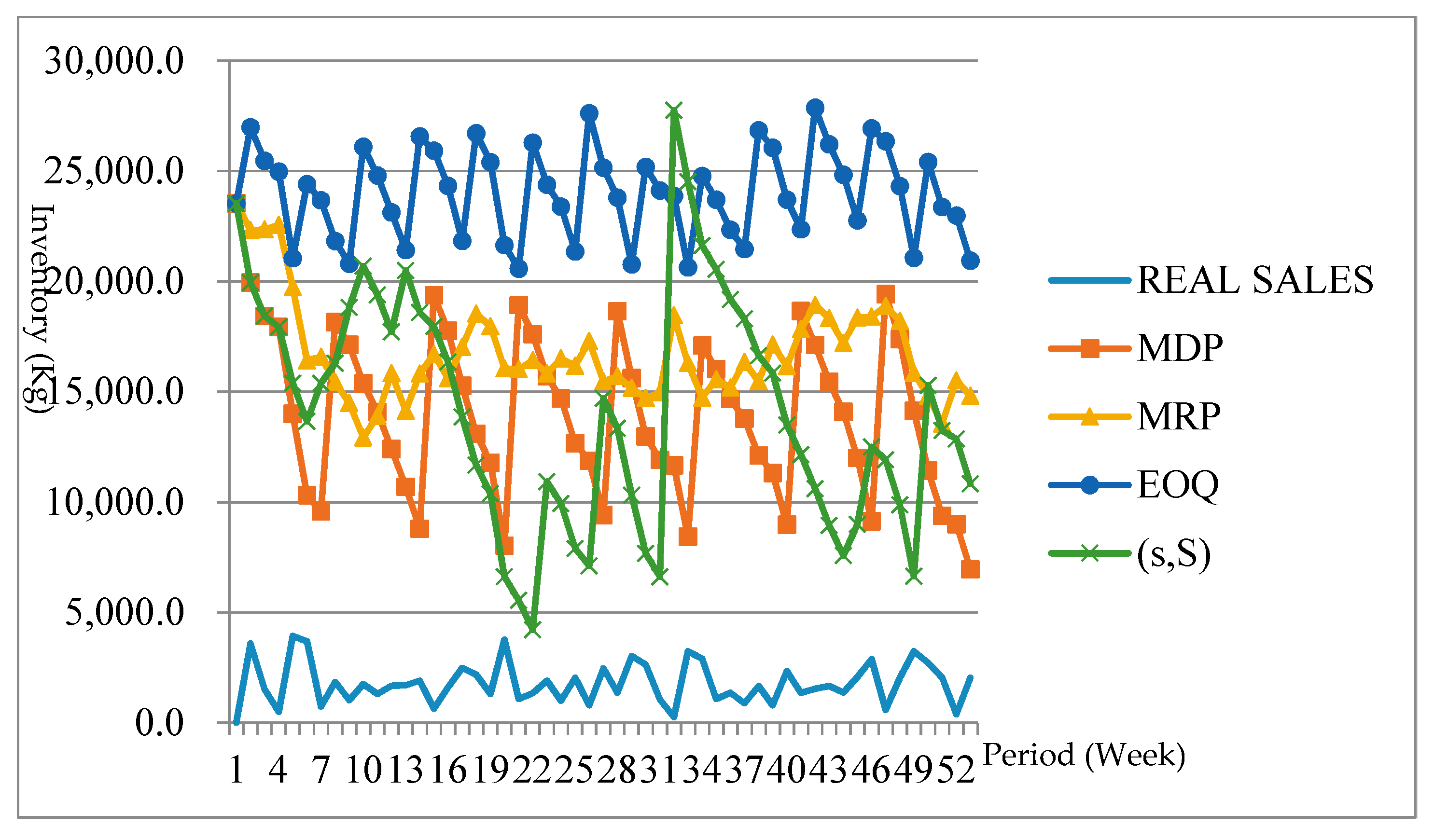
Table 1.
Basic data for product analyzed.
| Ending Inventory | Mean | Standard Deviation | Coefficient of Variation | |
|---|---|---|---|---|
| Item | ||||
| Real Item | 47,531.64 | 26,145.70 | 0.55 | |
Table 2.
States set.
| State | Low | Inventory | High |
|---|---|---|---|
| State 1 | −11,903.9 | ≤X< | 847.9 |
| State 2 | 847.9 | ≤X< | 13,599.7 |
| State 3 | 13,599.7 | ≤X< | 26,351.5 |
| State 4 | 26,351.5 | ≤X< | 39,103.3 |
| State 5 | 39,103.3 | ≤X< | 51,855.1 |
| State 6 | 51,855.1 | ≤X< | 64,606.9 |
| State 7 | 64,606.9 | ≤X< | 77,358.7 |
| State 8 | 77,358.7 | ≤X< | 90,110.5 |
| State 9 | 90,110.5 | ≤X< | 102,862.3 |
| State 10 | 102,862.3 | ≤X<= | 115,615.1 |
Table 3.
Rewards interval for each action.
| Action1 | Low | High | Action2 | Low | High | Action3 | Low | High |
|---|---|---|---|---|---|---|---|---|
| State 1 | 19,152.1 | 31,903.9 | State 1 | 49,152.1 | 61,903.9 | State 1 | 99,152.1 | 111,903.9 |
| State 2 | 6400.3 | 19,152.1 | State 2 | 36,400.3 | 49,152.1 | State 2 | 86,400.3 | 99,152.1 |
| State 3 | 0 | 6400.3 | State 3 | 23,648.5 | 36,400.3 | State 3 | 73,648.5 | 86,400.3 |
| State 4 | 0 | 0 | State 4 | 10,896.7 | 23,648.5 | State 4 | 60,896.7 | 73,648.5 |
| State 5 | 0 | 0 | State 5 | 0 | 10,896.7 | State 5 | 48,144.9 | 60,896.7 |
| State 6 | 0 | 0 | State 6 | 0 | 0 | State 6 | 35,393.1 | 48,144.9 |
| State 7 | 0 | 0 | State 7 | 0 | 0 | State 7 | 22,641.3 | 35,393.1 |
| State 8 | 0 | 0 | State 8 | 0 | 0 | State 8 | 9889.5 | 22,641.3 |
| State 9 | 0 | 0 | State 9 | 0 | 0 | State 9 | 0 | 9889.5 |
| State 10 | 0 | 0 | State 10 | 0 | 0 | State 10 | 0 | 0 |
Table 4.
Economic order quantity (EOQ) model.
| Input Dataset | |||
|---|---|---|---|
| Item | Holding Cost | Fixed Cost | Year of Demand |
| B | 132.76 | 35,000 | 110,726 |
Q * =7640.86.
Table 5.
(s,S) policy.
| Input Dataset | ||||||
|---|---|---|---|---|---|---|
| Item | Holding Cost | Fixed Cost | Lead Time | Mean of Demand | Variance of Demand | Service Level |
| B | 132.76 | 35,000 | 12 | 1675.1 | 1258.42 | 0.95 |
S = 28,211.5. s = 27,271.7
Table 6.
Optimal policy.
| Period | States | 1–43 | 44–46 | 47–49 | 50 | 51–52 |
|---|---|---|---|---|---|---|
| Optimal Actions | state 1 | 3 | 3 | 2 | 2 | 2 |
| state 2 | 3 | 2 | 2 | 1 | 1 | |
| state 3 | 3 | 2 | 1 | 1 | 1 | |
| state 4 | 3 | 2 | 1 | 1 | 1 | |
| state 5 | 2 | 2 | 1 | 1 | 1 | |
| state 6 | 2 | 2 | 1 | 1 | 1 | |
| state 7 | 2 | 2 | 1 | 1 | 1 | |
| state 8 | 2 | 1 | 1 | 1 | 1 | |
| state 9 | 2 | 1 | 1 | 1 | 1 | |
| state 10 | 1 | 1 | 1 | 1 | 1 |
© 2019 by the authors. Licensee MDPI, Basel, Switzerland. This article is an open access article distributed under the terms and conditions of the Creative Commons Attribution (CC BY) license (http://creativecommons.org/licenses/by/4.0/).
Share and Cite
MDPI and ACS Style
Tseng, S.-H.; Yu, J.-C. Data-Driven Iron and Steel Inventory Control Policies. Mathematics 2019, 7, 718. https://doi.org/10.3390/math7080718
AMA Style
Tseng S-H, Yu J-C. Data-Driven Iron and Steel Inventory Control Policies. Mathematics. 2019; 7(8):718. https://doi.org/10.3390/math7080718
Chicago/Turabian StyleTseng, Shih-Hsien, and Jia-Chen Yu. 2019. "Data-Driven Iron and Steel Inventory Control Policies" Mathematics 7, no. 8: 718. https://doi.org/10.3390/math7080718
Note that from the first issue of 2016, this journal uses article numbers instead of page numbers. See further details here.