Article

Sparse Recovery Algorithm for Compressed Sensing Using Smoothed l0 Norm and Randomized Coordinate Descent

1
Central South University, CAD/CAM Institute, Changsha 410075, China
2
Zhengzhou Railway Vocational & Technical College, College of Railway Engineering, Zhengzhou 450000, China
3
Zhengzhou Railway Vocational & Technical College, Department of Foreign Affairs & Scientific Research, Zhengzhou 450000, China
*
Author to whom correspondence should be addressed.
Mathematics 2019, 7(9), 834; https://doi.org/10.3390/math7090834
Submission received: 12 August 2019 / Revised: 3 September 2019 / Accepted: 6 September 2019 / Published: 9 September 2019
(This article belongs to the Section Engineering Mathematics)

Abstract

:
Compressed sensing theory is widely used in the field of fault signal diagnosis and image processing. Sparse recovery is one of the core concepts of this theory. In this paper, we proposed a sparse recovery algorithm using a smoothed l0 norm and a randomized coordinate descent (RCD), then applied it to sparse signal recovery and image denoising. We adopted a new strategy to express the (P0) problem approximately and put forward a sparse recovery algorithm using RCD. In the computer simulation experiments, we compared the performance of this algorithm to other typical methods. The results show that our algorithm possesses higher precision in sparse signal recovery. Moreover, it achieves higher signal to noise ratio (SNR) and faster convergence speed in image denoising.

1. Introduction

In recent years, compressed sensing (CS) has become an essential mathematical tool in the field of information theory [1,2]. It has been widely used in the field of fault diagnosis [3], image processing [4], data compression [5,6], and so on. CS theory suggests that a signal can be recovered from fewer samples than suggested by the Shannon–Nyquist sampling rate given that the original signal is sparse or approximately sparse in certain representation domains.
As shown in Figure 1, assuming that signal f (n × 1) will be recovered from incomplete sampling values, the sampled value of the signal f is as follows:
y = Φ f
where Φ (m × n, m << n) is the measurement matrix, and y (m × 1) is an measurement vector. When the dimension of y is much lower than that of f, Equation (1) becomes an underdetermined equation and f is unable to be calculated. However, if the number of non-zero elements in f is K (Km), f can be calculated, in which case K is called sparsity.
Most natural signals are not sparse in practical applications. The sparse representation of f is obtained by a specific mathematical transformation Ψ, as shown in Equation (2) and Figure 2.
f = Ψ s
where Ψ is the sparse dictionary, and s is the sparse representation coefficient, such that signal f can then be recovered indirectly by constructing the sparse coefficients, which is shown in Equation (3) and Figure 3.
y = Φ Ψ s
Here we set A = ΦΨ, then Equation (3) changes to y = As. If A satisfies restricted isometry property (RIP), s can be accurately recovered [1].
The CS theory consists of two parts. The first is the sparse representation. Because a natural signal is not sparse in a usual case, we need to first make it sparse by mathematical transformation. The second is sparse recovery, which means to recover the sparse signal. Among the two parts, the sparse recovery method directly determines the quality of signal recovery [7]. In this paper, we focus on proposing a sparse recovery algorithm for CS. In the following sections, signal s is set to be a sparse signal vector.
Generally speaking, the purpose of sparse recovery is to solve the l0 norm minimization problem, as shown in Equation (4):
{ min s 0 s . t .     y = A s
Equation (4) aims at seeking the minimal s 0 solution of y = A s , which is also called the (P0) problem. However, if m << n, the (P0) problem becomes the NP-hard, which means that we cannot solve Equation (4) directly in that condition [8,9,10].
One way to solve such (P0) problems are greedy algorithms, which include matching pursuit (MP) [11], orthogonal matching pursuit (OMP) [12], stage-wise orthogonal matching pursuit (StOMP) [13], compressive sampling matching pursuit (CoSaMP) [14], subspace pursuit (SP) [15], gradient pursuit (GP) [16], and so on. These algorithms are widely used in sparse recovery, but there are strict requirements for the sparsity. For instance, the OMP algorithm, only when K < n or A satisfies certain conditions, s can be recovered successfully [10].
In addition, we considered the following optimization problem:
{ min s p p s . t .     y = A s
According to the literature [10], there are notably different properties of lp norms for different values of p. As is shown in Figure 4, when p > 1, Equation (5) is a convex optimization problem and its solution is not sparse (the elements of the intersection point are all not 0). While when 0 ≤ p < 1, it becomes a non-convex optimization problem and its solution is sparse (only one element of the intersection point is 0). In particular, when p = 1, Equation (5) is called a basis pursuit (BP) algorithm and under certain conditions its solution is also sparse, but may not result in the sparsest solution compared to the case when 0 ≤ p < 1 [9].
In a term, if 0 ≤ p < 1, the solution of Equation (5) is more sparse. Unfortunately, this results in a non-convex optimization problem. In order to resolve this problem, researchers adopt the sum of a set of smooth concave functions to express the (P0) problem approximately, which is called the smooth l0 norm approximation algorithm.
For instance, literature [17] adopted an arctangent function as
f ( s i ) = π 2 arctan ( s i 2 2 σ )
where si is the elements in vector s. Then the (P0) problem can be approximately expressed as
{ min i = 1 n π 2 arctan ( s i 2 2 σ ) s . t .     y = A s
Similarly, some research [18] adopted a hyperbolic tangent function as
f ( s i ) = exp ( s i 2 2 σ 2 ) exp ( s i 2 2 σ 2 ) exp ( s i 2 2 σ 2 ) + exp ( s i 2 2 σ 2 )
The recovery algorithm based on a smoothed l0 norm and modified Newton method (L0MN) in the literature [19] adopted a function as
f ( s i ) = σ s i + σ
The recovery algorithm based on a smoothed l0 norm and gradient projection (L0GP) in the literature [20] adopted a function as
f ( s i ) = | s i | 2 | s i | 2 + σ 2
The smooth l0 norm approximation algorithms can be easily solved by Lagrange multiplier technique. However, because f(si) is non-convex, these algorithms have the possibility of falling into a local optimum.
In this paper, we have improved Equation (9) to establish a new strategy to express the (P0) problem approximately. However, the resulting optimization problem is still not a convex problem, hence finding a global optimal solution is not a trivial. For this, we selected a randomized coordinate descent (RCD) algorithm for solving the optimization, which does not guarantee one to find the global optimum, but it can avoid many local minima, and probably can land close to the global optimum.

2. Sparse Recovery Algorithm

2.1. Cost Function

Observing Equation (9), we find that it is a function with very simple structure. According to the literature [19], this equation can reduce the computational complexity while ensuring precision. However, as is shown in Figure 5, in very few cases, s i + σ = 0 will occur. This case can lead to the discontinuity of functions, which will affect the calculation results to a certain extent.
In order to avoid this defect, we give a continuous smooth fractional function as Equation (11),
f σ ( s i ) = σ s i 2 + σ
where σ > 0 . In this way, we guarantee the continuity of this function, which is shown in Figure 6.
As shown in Figure 7, when the value of σ decreases gradually, f σ ( s i ) gradually approaches the form of l0 norm, that is:
lim σ 0 f σ ( s i ) = { 1 ,     s i = 0 0 ,     s i 0
It should be noted that when σ 0 , although f σ ( s i ) and l0 norm look similar, they are essentially different. In order to use Equation (12) to express the (P0) problem, we make the following attempts:
{ min i = 1 n f σ ( s i ) s . t .     y = A s
As is shown in Equation (11), when σ 0 , the value f σ ( s i ) can only be 0 or −1. If we want to minimize i = 1 n f σ ( s i ) , we need to make as many terms as possible in this polynomial equal to −1. Then, according to Equation (11), this is equivalent to that which we need to make as many elements as possible in vector s equal to 0. Thus, this is consistent with the meaning of l0 norm minimization.
In a word, when σ 0 , the optimal solution of Equations (4) and (13) are identical. Therefore, we can adopt Equation (13) to express the (P0) problem approximately.
Equation (13) is a typical optimization problem with an equality constraint. The Lagrange multiplier method can transform such problems into unconstrained optimization problems. The cost function can be constructed as follows,
min L ( s ) = 1 2 A s y 2 2 + λ i = 1 N f σ ( s i )
where λ is the regularization parameter.

2.2. Solution

Generally, the gradient descent method (or the idea of gradient descent) can be used to solve Equation (14). The procedures of gradient descent method are as follows:
The gradient L ( s ) of L ( s ) at point s is:
L ( s ) = L s = A T ( A s y ) + λ ( f s 1 , f s 2 , , f s n ) T = A T ( A s y ) + λ ( 2 σ s 1 ( σ + s 1 2 ) 2 , 2 σ s 2 ( σ + s 1 2 ) 2 , , 2 σ s n ( σ + s 1 2 ) 2 ) T
If we want to minimize L ( s ) , we need to update s to the direction of negative gradient:
s ( k + 1 ) = s ( k ) h [ L ( s ( k ) ) ]
where h is the step size of the iterative process. When the initial value and termination condition are given, the optimal solution of Equation (14) can be obtained by iteration, and that is the standard gradient descent method.
However, the gradient descent method is not intended for non-convex problems, because it is easy to be trapped in local minima. Therefore, we need to adopt strategies to get it out of local minima. The common methods for this include the simulated annealing (SA) algorithm [21], the genetic algorithm (GA) [22], the randomized coordinate descent (RCD) [23] method, and so on. RCD is a special case of stochastic gradient descent (SGD) [24], which is widely used to optimize non-convex problems because of its simple principle and fast convergence speed.
Unlike the traditional gradient descent method, RCD adds random factors to the calculation of gradient. Therefore, even if it falls into the local minima, its gradient may not be zero, so it may jump out of the local minima and continue to iterate [23].
In each iteration process, RCD method does not derive partial derivatives of all variables, but derives partial derivatives of one (or several) variables. The detailed measures are as follows:
Let srand be a random element in vector s, and then we can calculate the gradient, as in Equation (17).
s rand L ( s ) = L s | s rand = a rand T ( A s y ) + λ ( 0 , , f s rand , , 0 ) T = a rand T ( A s y ) + λ ( 0 , , 2 σ s rand ( σ + s rand 2 ) 2 , , 0 ) T
where arand denotes the column corresponding to srand in matrix A. Then Equation (16) can be updated as:
s ( k + 1 ) = s ( k ) h [ s rand L ( s ( k ) ) ]
Now, we discuss how to choose the step size h. In the process of iteration, the value of the function is required to decrease, which is shown as Equation (19).
L [ s ( k + 1 ) ] < L [ s ( k ) ]
That is to say, when the direction of iteration is determined, we need to minimize L [ s ( k + 1 ) ] . This problem can be reduced to Equation (20).
{ min φ ( h ) s . t .     0 h h ( max )  
where φ ( h ) = s ( k ) h [ s rand L ( s ( k ) ) ] , and h ( max ) = 2 ( | s ( k ) T s ( k ) | ) 1 . Here we adopt Goldstein method to solve this problem, which can be referred to in the literature [25].
Because our method is to solve the smooth l0 norm based sparse recovery problem using RCD, we name it L0RCD.

2.3. Algorithm Description

Now, we summarize the sparse recovery algorithm in this paper, as in Table 1.
In Table 1, σ 0 and s0 are the initial values of σ and s, respectively. AT(AAT)−1y is the least square solution of y = As, and λ can be estimated by generalized cross-validation (GCV) method [26]. According to literature [17,18,19,20], in order to ensure that the search scope is more and more refined in the iteration process, we take a set of descending sequences of σ , where σ ( k + 1 ) = 0.7 σ ( k ) .

2.4. Computational Cost Analysis

The main computational complexity of L0RCD lies in the product of the vectors, as well as the calculation of partial derivatives in the iterative process. The computational burden of a rand T ( A s y ) is O(m2), while the burden of A T ( A s y ) is O(n2m). In addition, in the iteration process, our method only derives partial derivatives of one variable, while the general gradient descent methods derive partial derivatives of all variables. This means that, in a single iteration, the computational complexity of our method is much less than that of the general gradient descent method. Although adopting RCD will result in more iterations, its computational burden may still be lower [23].

3. Comparative Experiment

In this section, we will test the performance of the sparse recovery algorithms in the field of signal recovery and image denoising. All of the experiments are implemented in MATLAB R2012a on a personal computer with a 2.59 GHz Intel Pentium dual-core processor and 2 GB memory running the Microsoft Windows XP operating system.

3.1. Signal Recovery Experiment

In this section, for matrix A, we adopt a Gaussian random matrix with variance of 1, where the sizes of A are m × n, and m < n. The size of the sparse vector s is n × 1, and the 0 elements distribute randomly in s. The values of non-zero elements in vector s are also random. Vector y can be calculated by y = A s . Under the condition that y and A are known, we reconstruct s using the sparse recovery algorithm; the recovery result is denoted as s*.
Here we use precision to evaluate the performance of the algorithms. The precision is defined as follows:
p r e c i s i o n = 1 s s * 2 s 2

3.1.1. Comparison of RCD and the Modified Newton Method

In order to highlight the advantages of RCD, we compared it with the modified Newton (MN) method from the literature [19]. In addition, to give a fair comparison, we constructed the same l0 norm approximation by Equation (9). That is, we adopted the same cost function but different optimization methods in the signal recovery experiments of this section.
In the first experiment, m = 60 and n = 100 were fixed, and K varied between 5 and 40. The precisions are given in Figure 8.
From Figure 8, we see that when K ≤ 20, both RCD and MN can be used to recover s precisely. However, with the increase of K, RCD performs relatively better than MN. This shows that RCD is more appropriate under these conditions.
In the second experiment, K = 20 and n = 100 were fixed, and m varied from between 30 and 90. The precisions are given in Figure 9.
From Figure 9, we can see that when m ≥ 55, both the two methods perform well. However, with the decrease of m, RCD performs relatively better than MN.

3.1.2. Comparison of L0RCD and the Other Sparse Recovery Algorithms

In this section, we will compare the L0RCD with OMP, MP, basis pursuit(BP), and L0GP. Similarly to the first experiment, m = 60 and n = 100 were fixed, and K varied between 5 and 40. The precision of the five methods are given in Figure 10. From Figure 10, we see that with the increase of K, L0RCD performs better than the other four algorithms in precision.
In the second experiment, K = 20 and n = 100 are fixed, and m varies from between 30 and 90. The precision of the five methods are given in Figure 11. From Figure 11, we see that with the decrease of m, L0RCD performs better than the other four algorithms in precision.
In the rest of this subsection, we give a rough analysis for these sparse recovery algorithms. From Figure 10 and Figure 11, we find that when K ≤ 10 or m ≥ 65, the precision of the five algorithms are all 1 (or very close to 1). For the pursuit algorithms (OMP, MP and BP), they have stricter requirements for sparsity and measurements.
Here we do not intend to claim that the approximate l0 norm algorithms are “better” than the pursuit algorithms. In fact, approximate l0 norm algorithms need to appropriate parameters, and this often requires experience or a large number of repeated tests. In comparison, when the sparsity or measurements meet the requirements, the application of pursuit algorithms is more mature. For instance, the MOD (method of optimal directions) and K-SVD (K-singular value decomposition) used for the sparse representation of signals both employ the pursuit algorithms to implement sparse coding [10].

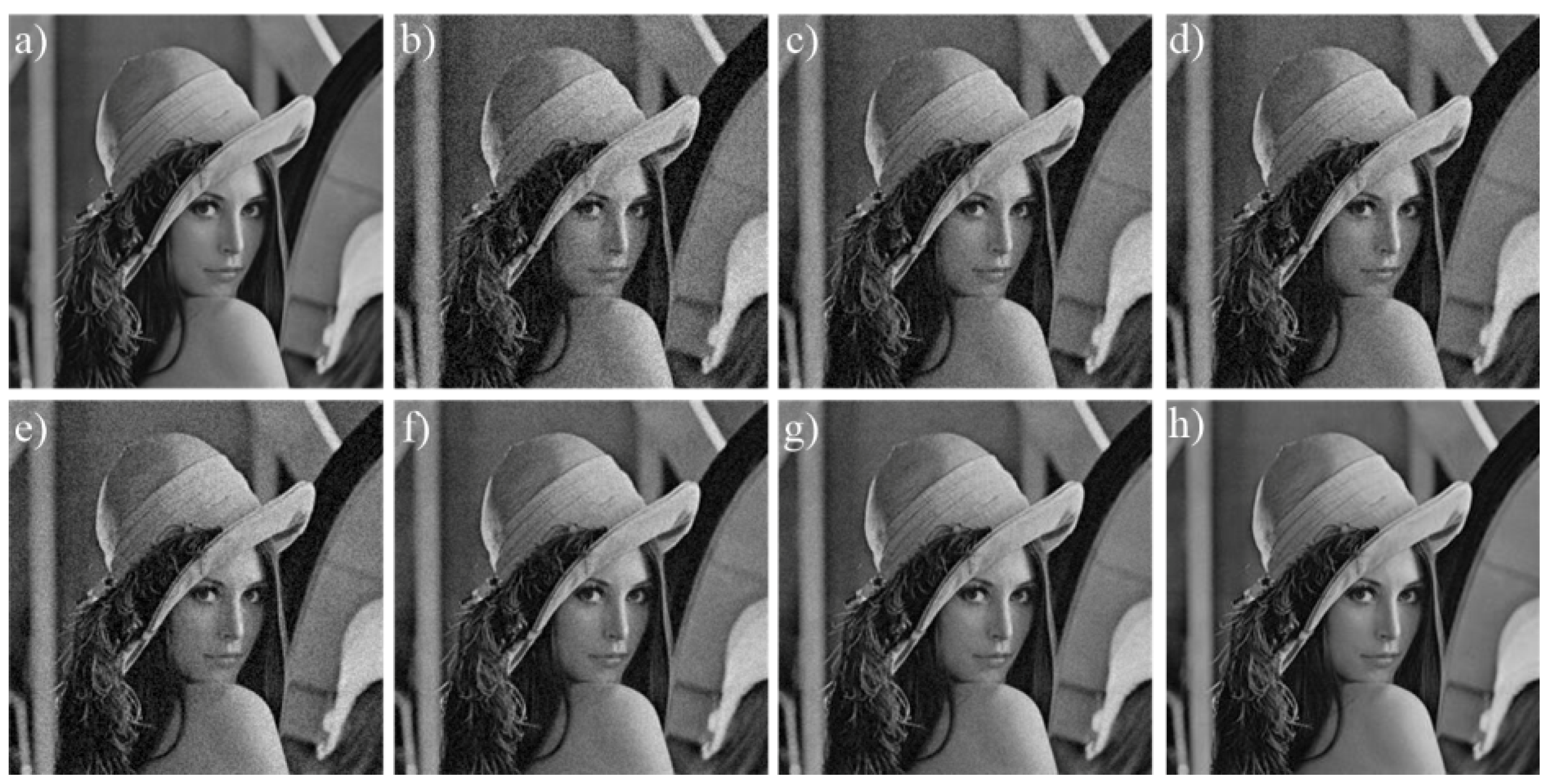
3.2. Image Denoising Experiment

When sparse recovery algorithm is applied to image denoising [27], Equation (4) should be changed to:
{ min s 0 s . t .   y A s 2 2 ϵ
where ϵ is a parameter related to noise level. The solution method of it is the same as that of (P0) problem, and y A s 2 2 ϵ can be regard as the relaxation of y = A s . According to literature [10], the pursuit algorithms are all applicable to Equation (22).
For approximate l0 norm method algorithms, the cost function for Equation (22) can be established as:
min ( s ) = 1 2 A s y 2 2 + λ s 0
In this section, we compared the image denoising performance of these methods under the same experimental conditions. We adopted signal to noise ratio (SNR) and time consumption to evaluate their performance, where SNR was defined as Equation (24).
SNR = 10 · lg i | s i | 2 i | s i * s i | 2
where s i * are the elements in s*. The higher the SNR, the better the image quality is.
We adopted three images named, respectively Lena, Cameraman, and Boat to test the denoising performance of the algorithms. The sizes of the three images are all 256 × 256 pixels. Gaussian noise with a mean of 0 and a standard deviation of 25 was added to the images.
Because an image is not a sparse signal, first, we used a two dimensional discrete cosine transform (2D-DCT) to represent these images sparsely. For matrix Φ, we adopted a Gauss random matrix with variance of 1, where the size of Φ was 128 × 256.
The intuitive denoising results are shown in Figure 12, Figure 13 and Figure 14. The SNR and time consumption are shown in Table 2.
From Figure 12, Figure 13 and Figure 14, we see that the image denoising performance of L0RCD is better than that of other five methods. From Table 2, we see that L0RCD only achieves higher SNR, but also consumes less time.

4. Conclusions

In this paper, a novel method based on RCD and approximate l0 norm is proposed to solve the optimization problem of sparse recovery. For the local minima defect of approximate l0 norm, we adopted a solution strategy with RCD. The simulations are carried out on sparse signal recovery and image denoising. Compared with the typical sparse recovery algorithms, our method performs better in precision. However, the success of the algorithm still depends on careful selection of the parameters, and how to overcome this defect is our further research goal.

Author Contributions

Conceptualization and writing, D.J.; project administration, G.Y.; funding acquisition, Z.L., software, H.L.

Funding

This research was funded by National Natural Science Foundation of China, grant number 61803086.

Acknowledgments

This research was supported by Yu.

Conflicts of Interest

The authors declare that there are no conflicts of interests regarding the publication of this paper.

References

  1. Donoho, D.L. Compressed sensing. IEEE Trans. Inf. Theory 2006, 52, 1289–1306. [Google Scholar] [CrossRef]
  2. Candes, E.J.; Wakin, M.B. An Introduction to Compressive Sampling. IEEE Signal Process. Mag. 2008, 25, 21–30. [Google Scholar] [CrossRef]
  3. Yuan, H.; Wang, X.; Sun, X.; Ju, Z. Compressive sensing-based feature extraction for bearing fault diagnosis using a heuristic neural network. Meas. Sci. Technol. 2017, 28, 065018. [Google Scholar] [CrossRef]
  4. Quan, T.M.; Nguyen-Duc, T.; Jeong, W.K. Compressed Sensing MRI Recovery Using a Generative Adversarial Network with a Cyclic Loss. IEEE Trans. Med. Imaging 2018, 37, 1488–1497. [Google Scholar] [CrossRef] [PubMed]
  5. Yi, S.; Cui, C.; Lu, J.; Wang, Q. Data compression and recovery of smart grid customers based on compressed sensing theory. Int. J. Electr. Power Energy Syst. 2016, 83, 21–25. [Google Scholar]
  6. Jin, D.; Yang, Y.; Luo, Y.; Liu, S. Lens distortion correction method based on cross-ratio invariability and compressed sensing. Opt. Eng. 2018, 57, 054103. [Google Scholar] [CrossRef]
  7. Ding, Y.; Selesnick, I.W. Artifact-Free Wavelet Denoising: Non-convex Sparse Regularization, Convex Optimization. IEEE Signal Process. Lett. 2015, 22, 1364–1368. [Google Scholar] [CrossRef]
  8. Lv, X.; Bi, G.; Wan, C. The Group Lasso for Stable Recovery of Block-Sparse Signal Representations. IEEE Trans. Signal Process. 2011, 59, 1371–1382. [Google Scholar] [CrossRef]
  9. Chen, S.S.; Donoho, D.L.; Saunders, M.A. Atomic Decomposition by Basis Pursuit. Siam Rev. 2001, 43, 129–159. [Google Scholar] [CrossRef] [Green Version]
  10. Elad, M. Sparse and Redundant Representations: From Theory to Applications in Signal and Image Processing; Springer: New York, NY, USA, 2010. [Google Scholar]
  11. Mcclure, M.R.; Carin, L. Matching pursuits with a wave-based dictionary. IEEE Trans. Signal Process. 1997, 45, 2912–2927. [Google Scholar] [CrossRef]
  12. Tropp, J.A.; Gilbert, A.C. Signal Recovery from Random Measurements Via Orthogonal Matching Pursuit. IEEE Trans. Inf. Theory 2007, 53, 4655–4666. [Google Scholar] [CrossRef]
  13. Donoho, D.L.; Tsaig, Y.; Drori, I.; Starck, J.L. Sparse Solution of Underdetermined Systems of Linear Equations by Stagewise Orthogonal Matching Pursuit. IEEE Trans. Inf. Theory 2012, 58, 1094–1121. [Google Scholar] [CrossRef]
  14. Karahanoglu, N.B.; Erdogan, H. A Orthogonal Matching Pursuit: Best-First Search for Compressed Sensing Signal Recovery. Digit. Signal Process. 2012, 22, 555–568. [Google Scholar] [CrossRef]
  15. Wei, D.; Milenkovic, O. Subspace Pursuit for Compressive Sensing Signal Recovery. IEEE Trans. Inf. Theory 2009, 55, 2230–2249. [Google Scholar]
  16. Vlachos, E.; Lalos, A.S.; Berberidis, K. Stochastic Gradient Pursuit for Adaptive Equalization of Sparse Multipath Channels. IEEE J. Emerg. Sel. Top. Circuits Syst. 2012, 2, 413–423. [Google Scholar] [CrossRef]
  17. Wang, J.H.; Huang, Z.T.; Zhou, Y.Y.; Wang, F.H. Robust sparse recovery based on approximate l0 norm. Acta Electron. Sin. 2012, 40, 1185–1189. [Google Scholar]
  18. Zhao, R.; Lin, W.; Li, H.; Hu, S. Recovery algorithm for compressive sensing based on smoothed l0 norm and revised Newton method. J. Comput.-Aided Des. Graph. 2014, 24, 478–484. [Google Scholar]
  19. Jin, D.; Yang, Y.; Ge, T.; Wu, D. A Fast Sparse Recovery Algorithm for Compressed Sensing Using Approximate l0 Norm and Modified Newton Method. Materials 2019, 12, 1227. [Google Scholar] [CrossRef]
  20. Wei, Z.; Zhang, J.; Xu, Z.; Huang, Y.; Liu, Y.; Fan, X. Gradient Projection with Approximate L 0 Norm Minimization for Sparse Recovery in Compressed Sensing. Sensors 2018, 18, 3373. [Google Scholar] [CrossRef]
  21. Bertsimas, D.; Tsitsiklis, J. Simulated Annealing. Stat. Sci. 1993, 8, 10–15. [Google Scholar] [CrossRef]
  22. Bender, M.A.; Muthukrishnan, S.; Rajaraman, R. Genetic algorithms: A survey. Computer 2002, 27, 17–26. [Google Scholar]
  23. Patrascu, A.; Necoara, I. Efficient random coordinate descent algorithms for large-scale structured nonconvex optimization. J. Glob. Optim. 2015, 61, 19–46. [Google Scholar] [CrossRef]
  24. Gardner, W.A. Learning characteristics of stochastic-gradient-descent algorithms: A general study, analysis, and critique. Signal Process. 1984, 6, 113–133. [Google Scholar] [CrossRef]
  25. Nocedal, J.; Wright, S.J. Numerical Optimization; Springer: Berlin, Germany, 2006. [Google Scholar]
  26. Lukas, M.A. Asymptotic optimality of generalized cross-validation for choosing the regularization parameter. Numer. Math. 1993, 66, 41–66. [Google Scholar] [CrossRef]
  27. Metzler, C.A.; Maleki, A.; Baraniuk, R.G. From Denoising to Compressed Sensing. IEEE Trans. Inf. Theory 2016, 62, 5117–5144. [Google Scholar] [CrossRef]
Figure 1. Incomplete sampling of signal f.
Mathematics 07 00834 g001
Figure 2. Sparse representation of signal f.
Mathematics 07 00834 g002
Figure 3. Basic principles of compressed sensing.
Mathematics 07 00834 g003
Figure 4. Properties of lp norms for different values of p.
Mathematics 07 00834 g004
Figure 5. Surface graph of σ / ( s i + σ ) .
Mathematics 07 00834 g005
Figure 6. Surface graph of σ / ( s i 2 + σ ) .
Mathematics 07 00834 g006
Figure 7. Diagram of σ / ( s i 2 + σ ) with different σ values.
Mathematics 07 00834 g007
Figure 8. Comparison of randomized coordinate descent (RCD) and modified Newton (MN) (changed K).
Mathematics 07 00834 g008
Figure 9. Comparison of RCD and MN (changed measurements).
Mathematics 07 00834 g009
Figure 10. Precision comparison of the five algorithms (changed K).
Mathematics 07 00834 g010
Figure 11. Precision comparison of the five algorithms (changed measurements).
Mathematics 07 00834 g011
Figure 12. Recovery effect of the six methods to the Lena image. (a) original image; (b) noisy image; (c) orthogonal matching pursuit (OMP); (d) stage-wise OMP (StOMP); (e) basis pursuit(BP); (f) l0 norm and gradient projection (L0GP); (g) l0 norm and modified Newton method (L0MN); (h) L0RCD.
Mathematics 07 00834 g012
Figure 13. Recovery effect of the six methods on the Cameraman image. (a) original image; (b) noisy image; (c) OMP; (d) StOMP; (e) BP; (f) L0GP; (g) L0MN; (h) L0RCD.
Mathematics 07 00834 g013
Figure 14. Recovery effect of the six methods on the Boat image. (a) original image; (b) noisy image; (c) OMP; (d) StOMP; (e) BP; (f) L0GP; (g) L0MN; (h) L0RCD.
Mathematics 07 00834 g014
Table 1. The description of the smooth l0 norm based sparse recovery algorithm using RCD (L0RCD).
Algorithm: L0RCD
Input:A, y, λ, h, K, and the termination condition: σ min = 10 3 σ 0 ;
Output: The recovery signal s*;
Initialization:s0 = AT(AAT)−1y, σ 0 = 1;
Step 1: Calculate gradient according to Equation 17;
Step 2: Iterate, s ( k + 1 ) = s ( k ) h [ s rand L ( s ( k ) ) ] ;
Step 3: If s ( k + 1 ) s ( k ) 2 σ , update s and σ , where σ ( k + 1 ) = 0.7 σ ( k ) , or else go to Step 1 and continue iterating.
Step 4: Take the updated s and σ as initial value, and repeat step 1 to step 3, stop iterating until σ < σ min and output to s*.
Table 2. The quantitative results (signal to noise ratio (SNR)/Time consumption(s)) of the six algorithms.
AlgorithmLenaCameramanBoat
OMP26.27/43.0225.98/44.5725.11/47.54
StOMP27.01/39.0727.33/42.1625.76/45.55
BP28.34/76.3728.97/78.3929.05/84.29
L0GP32.13/25.1433.14/27.3331.06/28.77
L0MN33.08/18.0434.59/20.2533.27/23.05
L0RCD34.95/17.1235.65/20.0134.05/21.86

