Abstract
Innovative solutions and techniques in the sports industry are commonly used and tested in real conditions. Elite athletes have to achieve their peak performance before the main competition of the year, which is the World Championship, and every fourth year before the Olympic Games, when the main competition of athletes takes place. The present study aims to analyze and evaluate the ability of elite kayakers to achieve the best form at the right times, with the Olympic Games taking the greatest importance. Target values for multiple measures of conditioning are compared to target values set by experts. A weighted least squares metric with weights varied by time period is developed as a measure of fulfillment of the athletes’ conditioning plans. The novelty of the paper is the idea of using linear combination of polynomials and trigonometric functions for approximating the target functions and application of the proposed methodology for the optimization and evaluation of athletic training.
1. Introduction
Sports are a phenomenon of global importance. The investment in professional athletes is a particularly important process. Sporting events promote the development of powerful worldwide industries. A key factor in sports is the ability to develop training schedules to optimize the athletes’ training conditions. The optimization and evaluation of athletic training is the most important problem for sports scientists, coaches, and athletes. Elite athletes are willing to perform more voluminous and high-quality training routines, and this process requires effective management. Elite athletes attain a world-class status in endurance sports after four to seven years of specialized training [1]. Over this period, they usually have 3000–7000 h of effective training and cover distances of 3000–4000 km/yr [2]. Winning medals in international competitions requires not only outstanding abilities and the long-term training of athletes, it is also crucial that they achieve peak performance at the right time.
The Olympic Games is the main competition for the Olympic sports athletes. There are four years of the Olympic training cycle, with its organizational structure and training methodology directed at making the successful start of athletes in the Olympic Games [3]. The elite athletes’ training must be carefully planned for several years in the future and based on individual indicators (training load specification and the athlete’s body adaptation to a particular training load). The process of the elite athletes’ training is complex and difficult to predict because of a number of unknown factors (i.e., accidents, acclimatization, illnesses, psychological changes, the pace of recovery, etc.) [4].
The Olympic training cycle consists of four one-year macro cycles, with the main competition, the World Championship, taking place in each of these cycles. The athletes make strenuous efforts to be in their best form before the World Championship. In the last year of the Olympic cycle, some of the athletes get a chance to participate in the Olympic Games during the World Championship. It means that athletes have to achieve their peak performance twice a year. In this case, the management of training is very complicated, because the athletes need to achieve their peak performance in a short time [5,6].
Monitoring the training load and athletes’ physiological adaptation is essential for optimizing training and minimizing the risk of overtraining, injuries, illnesses, etc. Usually, sports managers and scientists are restricted in publishing the data on the athletes’ condition before competitions. In elite sports, monitoring is extensive, but most of the data remain confidential [7].
Scientists are searching for novel approaches to visualize and analyze the data obtained in the training sessions. One of the most relevant research topics is visualization for motion analysis, which is important for training optimization, technical and tactical improvements, as well as the prevention of injuries [8]. However, not only motion optimization is required for achieving good results. The growing need causes the necessity for making a training process much more technologically advanced, and this is an important field of interest for athletes, coaches, and scientists. Massive amounts of data are generated and used in sports medicine, including preventative care and rehabilitation. Most major professional teams today make data-driven decisions and employ the analytical staff to help prepare training plans, predict athlete risks, and prescribe personalized recovery strategies. Most of the athletes use trackers to measure, accompany, and control the data (e.g., power, velocity, duration, altitude, and heart rate) obtained in training and later perform an individual analysis and online planning [9]. The present study focuses on the visualization of the training process based on the physiological condition of athletes.
The optimization of the athletic training process is an appropriate application of operational research (OR). Prediction management and decision making in athletic training should be based on objective data analysis and parameter estimation [10].
Reviewing the literature related to the application of mathematical models and methods used for solving similar problems has shown that the authors use various approaches. For example, Armstrong, Weidner, and Walker [11] have elaborated on the analysis of variance (ANOVA) and t-test of independent samples for clinical proficiency evaluation in athletic training. A qualitative analysis of the respondents’ comments has also been performed.
Li, Zhu, Chen, and Xue [12] have elaborated on the balanced approach of data envelopment analysis (DEA) to cross-efficiency evaluation. An iterative algorithm for obtaining the final optimal and balanced cross-efficiency score has been developed by the authors.
Four imbalance indicators for measuring the difference between standard distribution and the ideally balanced distribution have been proposed by Karsu and Morton [13]. The interesting phenomenon is the total componentwise proportional deviation because it is an individual-oriented measure, which is the weighted sum of fractional misallocations for each party.
The Delphi method has been used by Reefke and Sundaram [14] to identify a set of key sustainable supply chain management (SSCM) problems and the associated research opportunities. The data components have been synthesized, and the parameters have been estimated according to their relative importance based on the experts’ judgments. New insights into the potential dependencies between the factors and their influence on the success of SSCM have been provided in this work. The development of the schedule for the sporting activities of the Ecuadorian football federation under a set of constraints with the use of integer programming has been proposed by Recalde, Torres, and Vaca [15]. A heuristic three-phase approach has also been adjusted to solve the considered problem. The developed methodology provides more benefits than the empirical method.
Algorithms based on multiple criteria decision making are often used in solving various problems in sports management. Dadelo, Turskis, Zavadskas, and Dadelienė [16] have described a novel framework for practical assessment and the ranking of basketball players based on the adjusted well-known Technique for Order of Preference by Similarity to Ideal Solution (TOPSIS) method. The graphical visualization of similarities provides further insights [17,18]. Visualization solutions of processes are better understood, allowing one to intuitively select a more appropriate optimization method. The visualization of processes is particularly useful for the cases with a variety of large and small factors, which should be controlled [19]. This is particularly important for inexperienced (non-professional) users.
The present study aims to analyze the ability of elite kayakers to achieve peak performance at the right times, with the Olympic Games taking the greatest importance. Real data is collected from two Olympic kayakers, and regression analysis is used (a combination of polynomial and trigonometric functions) to model how well their conditioning fits the ideal. A weighted least squares metric with weights varied by time period is developed as a measure of fulfillment of the athletes’ conditioning plans.
In our knowledge, the proposed methodology for the first time was applied for sports management process optimization. However, the scope of the methodology is not limited to the field of athletic training analysis and optimization. Another challenge in this study is the limited amount of data available. The data of two athletes’ Olympic training cycles are available. In addition, the data are not independent, as both athletes compete in a pair. This complicates the application of other methods, such as statistical methods, to address this problem. Therefore, in this application, the visualization approach should be defined for monitoring the condition of top kayakers during the three-year macro cycles before the Olympic Games.
Except for the Introduction, the article is organized as follows. In Section 2, the description of the experiment and the measured and expected target values of the indicators set by experts are provided. Section 3 is focused on justifying the selection of the approximation function. In Section 4, the research methodology, based on the approximation of functions by using a linear combination of polynomials and trigonometric functions, is described, and the calculated unknown coefficients are given. Section 5 describes visualization of the approximation of the target and the measured functions, and presents a measure of the difference between the target and the measurement functions, which defines the athlete’s condition. Section 6 provides the discussion of the investigated problem and conclusions.
2. The Investigation Object and the Initial Data
2.1. The athletes’ Participation in the Study
The research was performed in the second, third, and the fourth year of the Olympic four-year cycle, at the time of athletic training for Rio de Janeiro Olympic Games in 2016. Two (1, 2) elite flat-water kayak paddlers (a racing team), performing at the international competitive level at the distance of 1000 m (whose ages were 27 and 26 years, and body mass were 88.5 and 84.5 kg, respectively), volunteered to take part in the investigation. These two athletes gained fifth place in a 1000 m event (K-2) in the 2016 Olympic Games in Rio de Janeiro.
2.2. The Description of the Experiment
A council, consisting of 22 Lithuanian kayaking elite experts (trainers and sports researchers), with no less than 10 years of experience in execution and organization in kayaking, have rated the competences and created the dynamics of the ideal curves of indicators based on correlations between indicators and sports outcomes [20].
The training volume and intensity were carefully controlled and quantified by using the Garmin Connect Forerunner 910 XT during each training session throughout the cycle. The data obtained from the devices were sent to three delegates from the sports science experts’ council, who are the creators of the athletes’ training programs. During the study, the athletes were encouraged to undertake their standard training sessions but not to train on the day before each test. The athletes were acquainted with the experimental procedures prior to testing and gave a written consent to participate in the study. All experimental procedures were approved by the Lithuanian Ethics Committee.
The testing lasted for three seasons (macro cycles): in each season, the training period lasted for 8 months, the competition period lasted for 3 months, and the transition period lasted for 1 month. Physiological testing of the athletes’ condition was performed at the Lithuanian University of Education Science. For each athlete, all tests were conducted at the same time of the day, between 09:00 and 11:00, and 24 h after the last training session. During the testing session, the tests were performed in the same order. Prior to beginning the study, the sports doctor examined the kayakers to exclude any medical disorders that could limit their participation in the investigation.
During the macro cycles (I, II, III), the athletes were tested in six periods of time: in (T1), in the first week of the introductory training period, in (T2), at the beginning of the general training period, in (T3), at the beginning of the specific training period, in (T4), at the beginning of the competitive training period, in (T5), at the beginning of the main competition period, and in (T6), at the time after the main competition period.
Standard methodologies were applied to determine the athletes’ physical parameters, i.e., their height (cm) and body mass (kg) [21].
The resting heart rate (b/min) was determined for each athlete in the supine position and in the period after the application of the standard physical load (30 squats within 45 s) by using the Garmin Connect Forerunner 910 XT.
Hemoglobin concentration (g/L) was determined by using a Hemocue analyzer. A trace amount of blood samples was taken from the fingertips of the athletes in the resting position.
The ergometer test was performed, using Oxycon Mobile 781023-052, version 5.2 (Cardinal Health Germany 234 GmbH, Höchberg, Germany). Gas analyzers were calibrated before and verified after each test. Each athlete performed the incremental submaximal ergometer test, using a calibrated kayak ergometer (Dansprint PRO, KE001 ergo, Hvidovre, Denmark) for determining the maximum oxygen uptake (VO2max) [22]. Five minutes before performing the submaximal ergometer test, the athletes completed a 15-min warm up. The incremental test began with the application of the initial workload of 100 W, and increments of 20 W were applied at the intervals of 30 s to bring the athlete to the limit of tolerance in 8–12 min. During the last minute, the athlete was encouraged to do as much work as he could. Then, the values were averaged over the intervals of 30 s. Pulmonary ventilation (PV) (1/min), oxygen uptake (VO2) (1/min, mL/min/kg), work capacity (W), and speed (km/h) were recorded at the point of the critical intensity limit (CIL).
For reaching the aim of the present study, all tests were arranged in hierarchical order by the experts’ board (from the most informative to the least informative indicator), which influenced the outcome of a sporting event, measured in percent (Table 1). In addition, all the testing sessions were also arranged in the hierarchical order. Their importance is shown in Table 2.

Table 1.
Test indicators presented in the hierarchical order set by the experts from the most to the least important indicator.

Table 2.
Importance of the testing sessions presented in the chronological order from the least (1) to the most (10) important session and their hierarchical order set by the experts.
In Table 3, the results of measurements of seven indicators for both athletes and the expected target values determined by the experts are presented. Here, denotes the athletes, is the number of the indicator, and is the number of the measurement. For example, . The expected target values differ for athletes 1 and 2 only in the case of because of the different lung volumes of the athletes.

Table 3.
Measurements of seven indicators for two athletes (the first row) and the expected target values (the second row).
3. The Selection of the Approximating Functions
The shape of the approximating functions was determined only for the target curves, which were created according to experts’ judgments. The available data were compared with the ideal (target) curves. The following factors were taken into account for the selection of the suitable functions for the curves:
- The approximation curve should not only describe the upward or downward trend, but also show the characteristic phase of the fall and the subsequent growth phase of the considered processes.
- The shape of the functions should be the same for all the curves and be simple enough. Its parameter values were determined by the least squares method.
Let us show how the ideal curve was constructed for the case of RN2. The values of the normalized data were as follows:
(0.0,1.0), (0.091,1.044), (0.186,1.094), (0.232,1.172), (0.290,1.150), (0.316,1.194), (0.346,1.056),
(0.438,1.094), (0.533,1.139), (0.576,1.167), (0.636,1.206), (0.663,1.222), (0.708,1.083), (0.788,1.128),
(0.857,1.167), (0.887,1.183), (0.976,1.239), (1.0,1.250).
The shape of the selected curve with the coefficients determined by the least squares method was as follows:
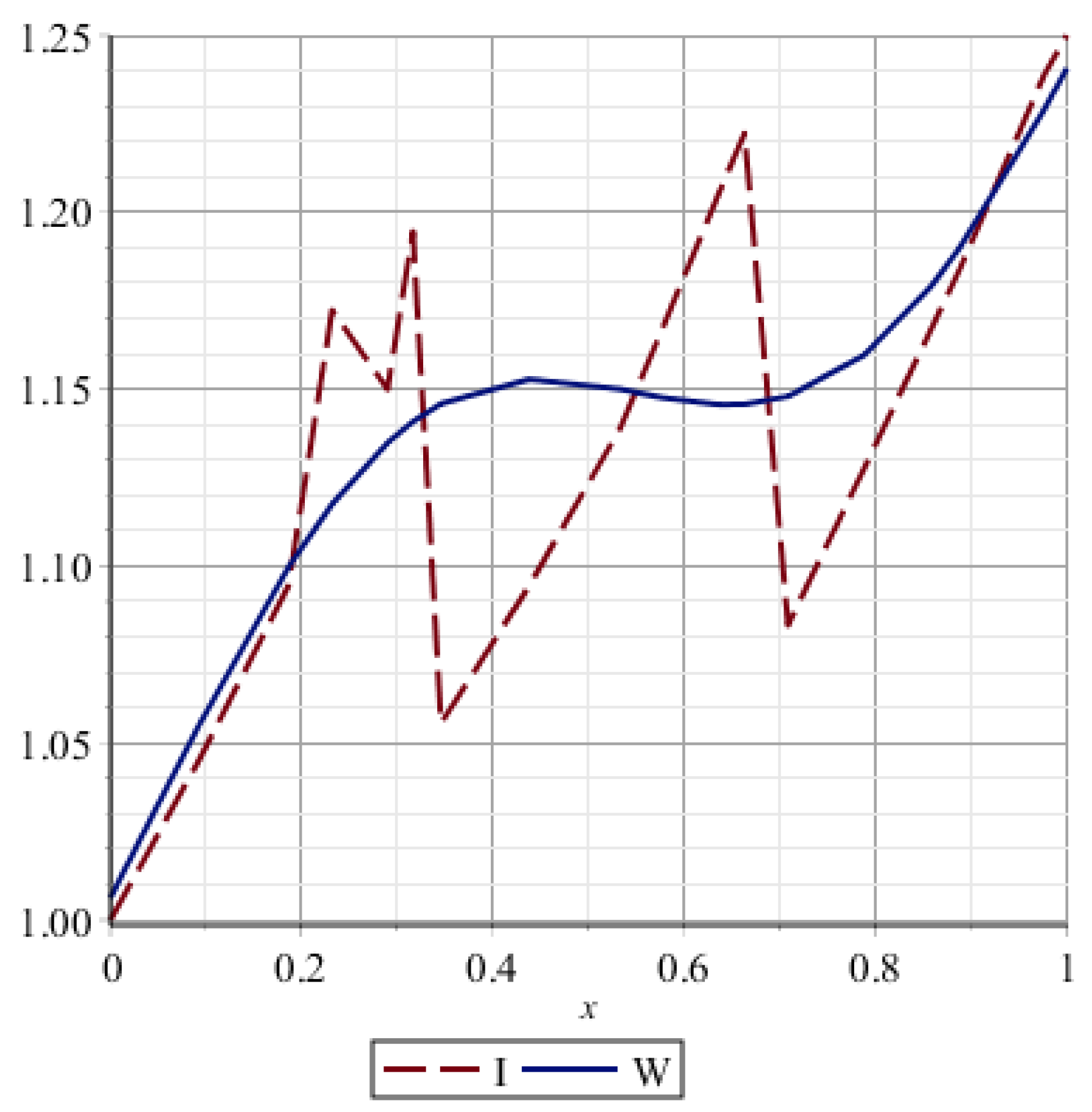
The curve and the linear interpolation of the points are depicted in Figure 1. Note that the graphical accuracy is sufficient for the purpose of the study, because the curve satisfies requirements 1 and 2. On the other hand, describing all the fluctuations of the linear interpolation does not make sense, because the similarity of these real data points can be hardly realized in practice. It should also be noted that the authors did not intend to construct the best curves, and therefore constructed the curves of sufficient approximation. However, other combinations of algebraic and trigonometric polynomials, which were acceptable, were also tested. The final decision about the choice of the formula was taken according to requirement 2 (the formula is appropriate for all the cases considered).

Figure 1.
Approximation of the target function .
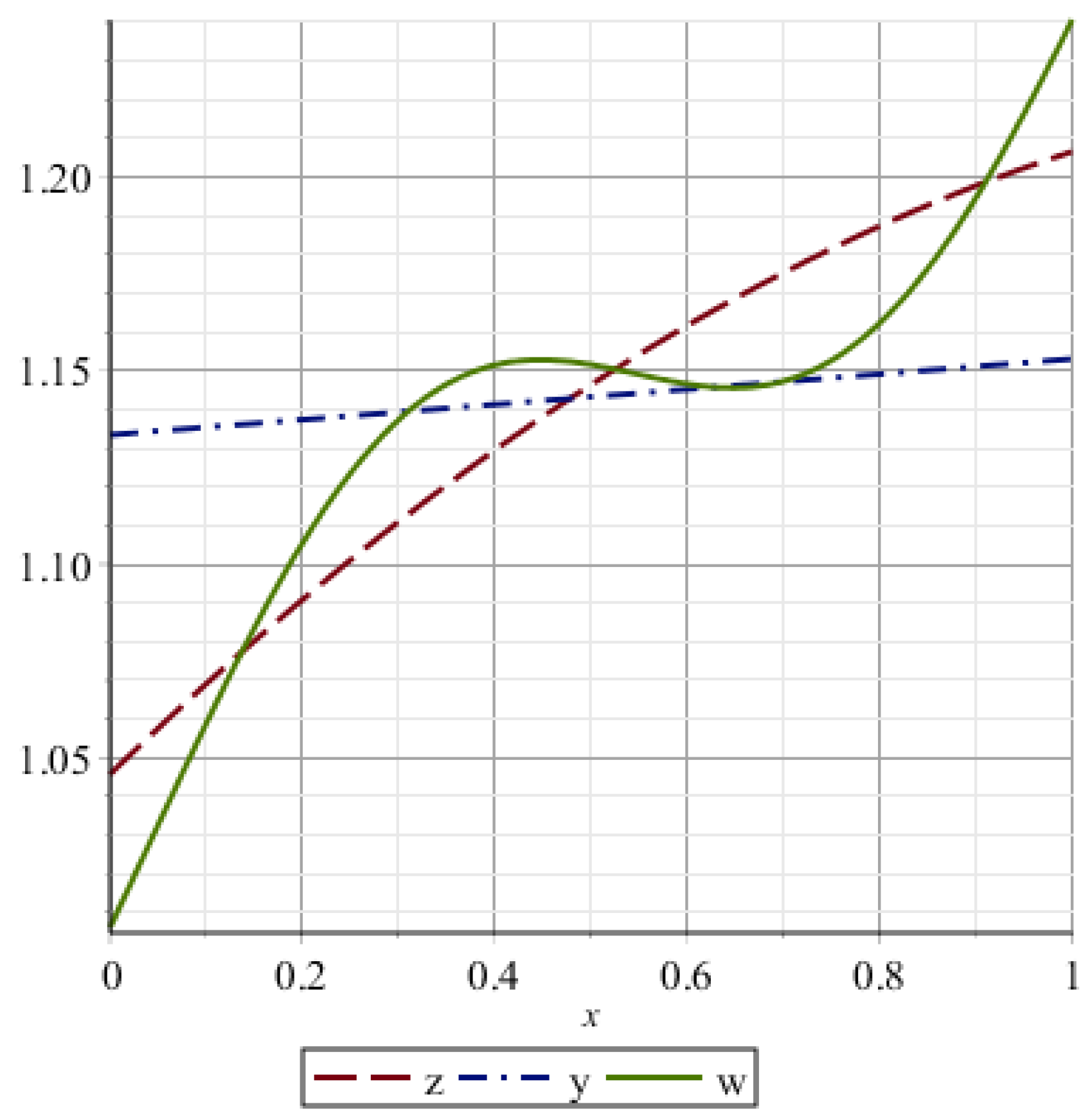
Figure 2 shows the functions
with the coefficients determined by the least squares method based on the same data. We can see that the curves and do not satisfy requirement 1. The values of the error function were calculated as follows:
where is equal to . The following error function values were obtained: . One can see that the best result was achieved by incorporating trigonometric components into the approximation function.

Figure 2.
Approximations of the target function .
4. Research Methodology
In the first step, all the initial data points (Table 3) were normalized to eliminate the influence of the measurement units on the final results. The values and were normalized by the equations:
This method of data normalization, when each measurement and target value were divided by the first target value of the respective measurement, was chosen for the convenience of data representation. In this case, the graphs of all the target values of the indicators have the same initial point of 1.
The measurement time was normalized as follows:
where is the number of days passed since the first measurement, . The respective values are shown in Table 4.

Table 4.
Normalized time values.
The goal was to find the functions most suitable for approximating the athlete’s indicators. The target values for a multiple measure of conditioning were compared to the targets set by the experts. The regression analysis was used to model how well their conditioning could fit the target. The weighted least square metric is a measure of the fulfillment of the athletes’ conditioning plans. The expression with five undefined coefficients, , was chosen for approximating the functions as follows:
where is the normalized time. The unknown coefficients were determined by a standard method of the least squares [23]:
The system of linear equations was obtained from Equations (1) and (2) as follows:
where
The coefficients were calculated by the equations:
where the functions obtained the values and , i.e., the coefficients were calculated separately for each athlete and each indicator for the functions and .
The matrix , depending only on the values , was calculated only once:
For calculating the coefficients the inverse matrix method is convenient to use (see, for example, [24]):
In Table 5, the values of the coefficients which were calculated by Equation (3), are presented for for the functions and.

Table 5.
Calculated values of the coefficients.
5. Visualization of the Results and Measurement of the Athlete’s Condition
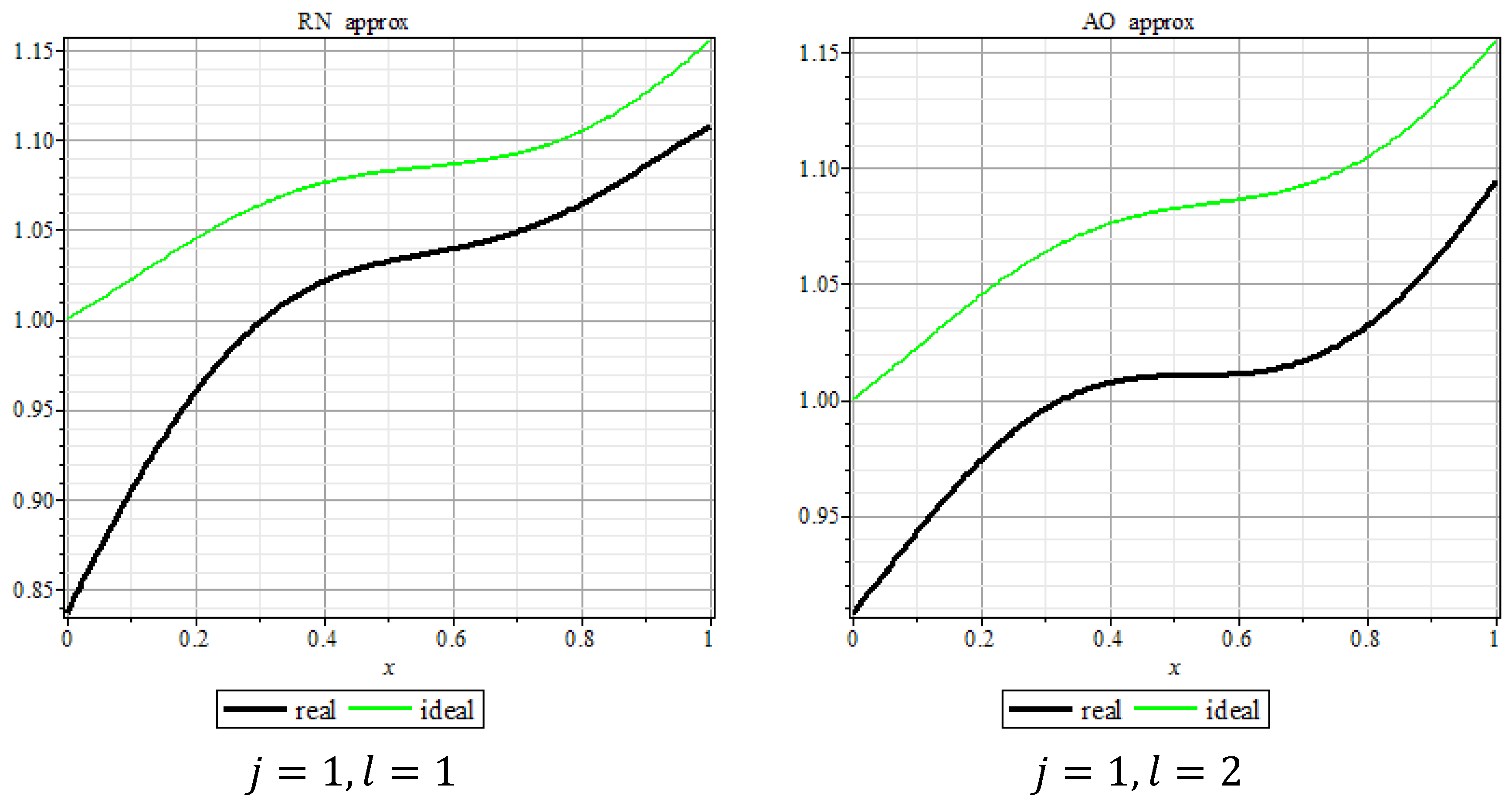
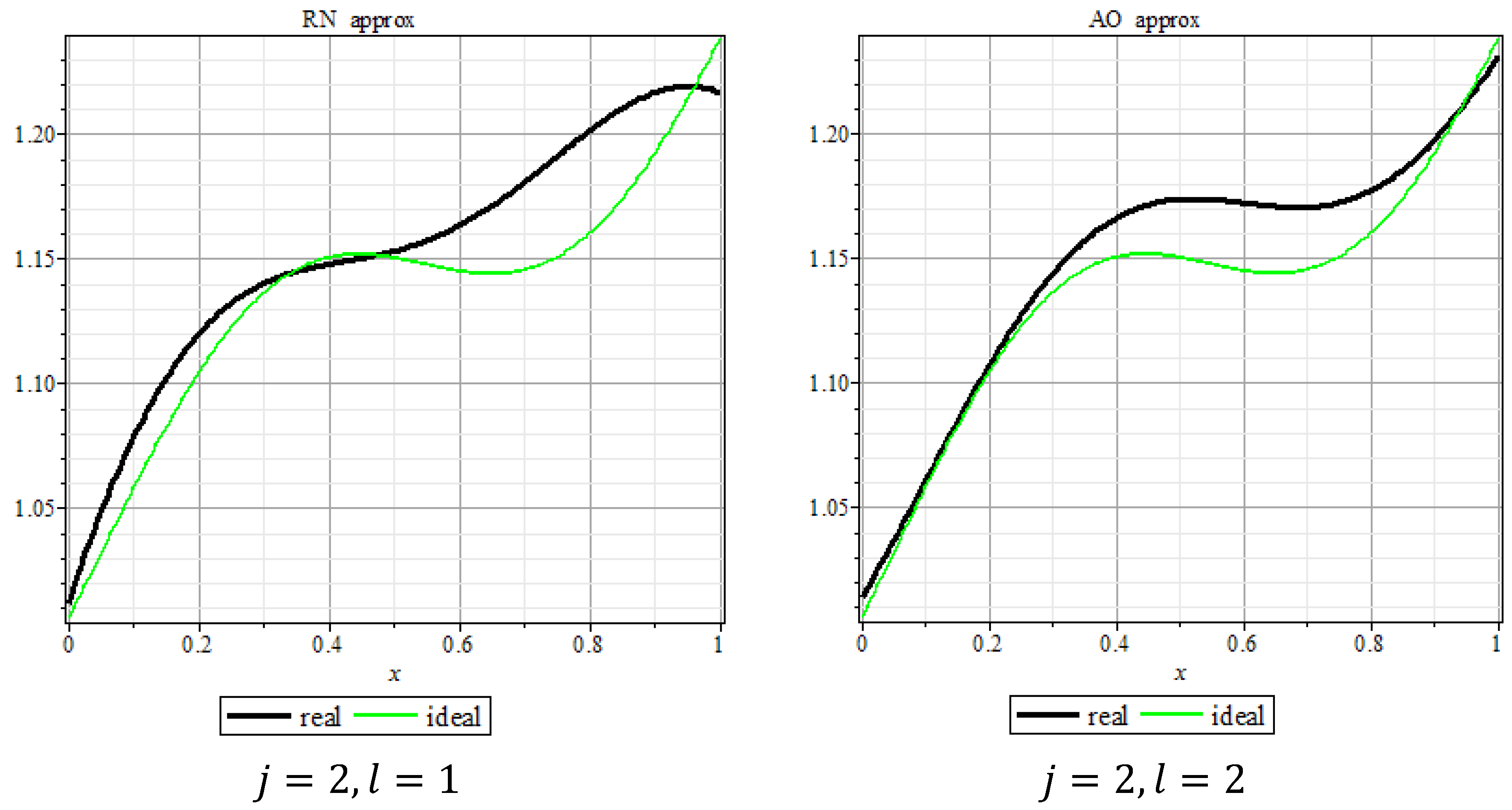
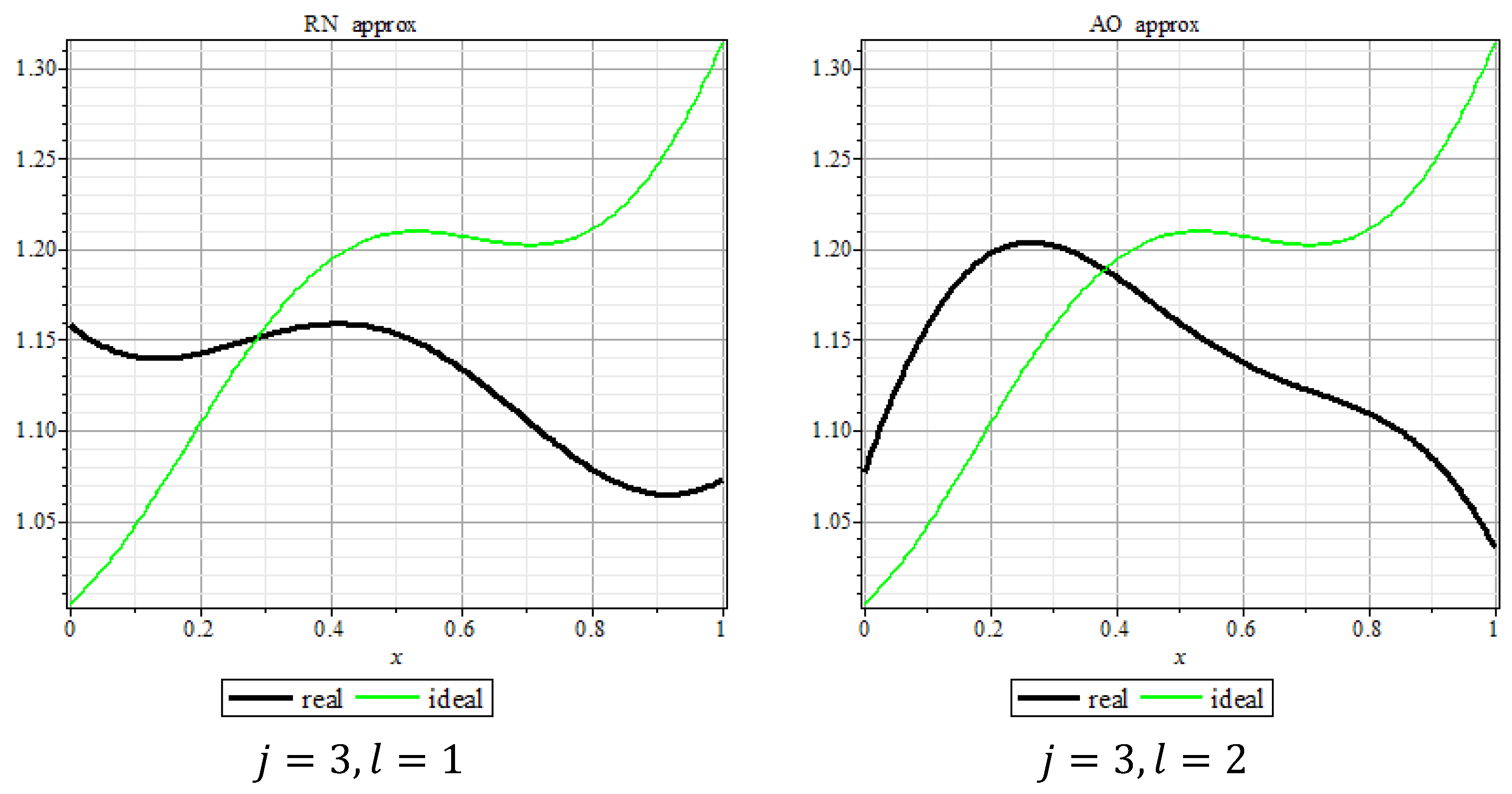
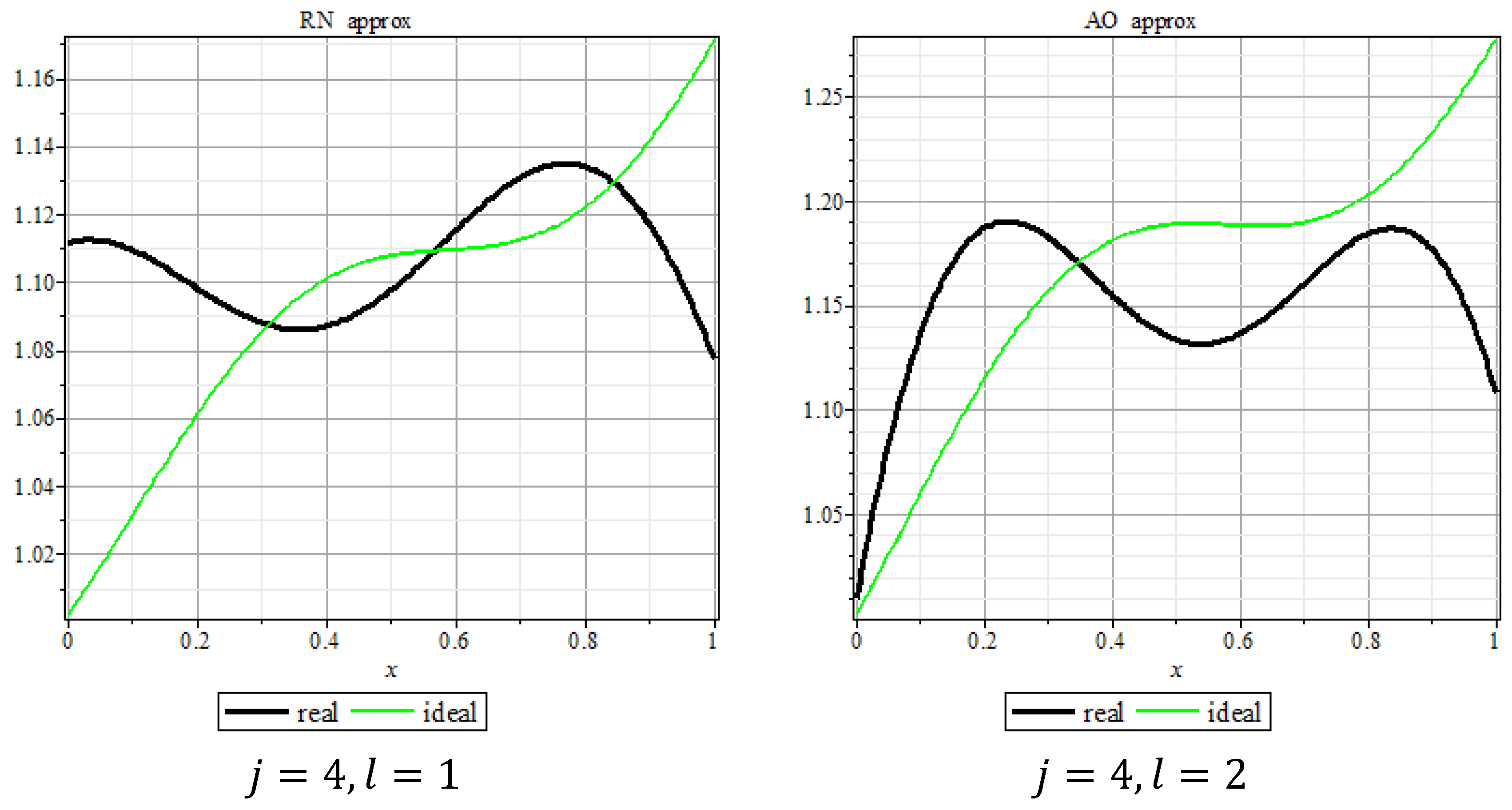
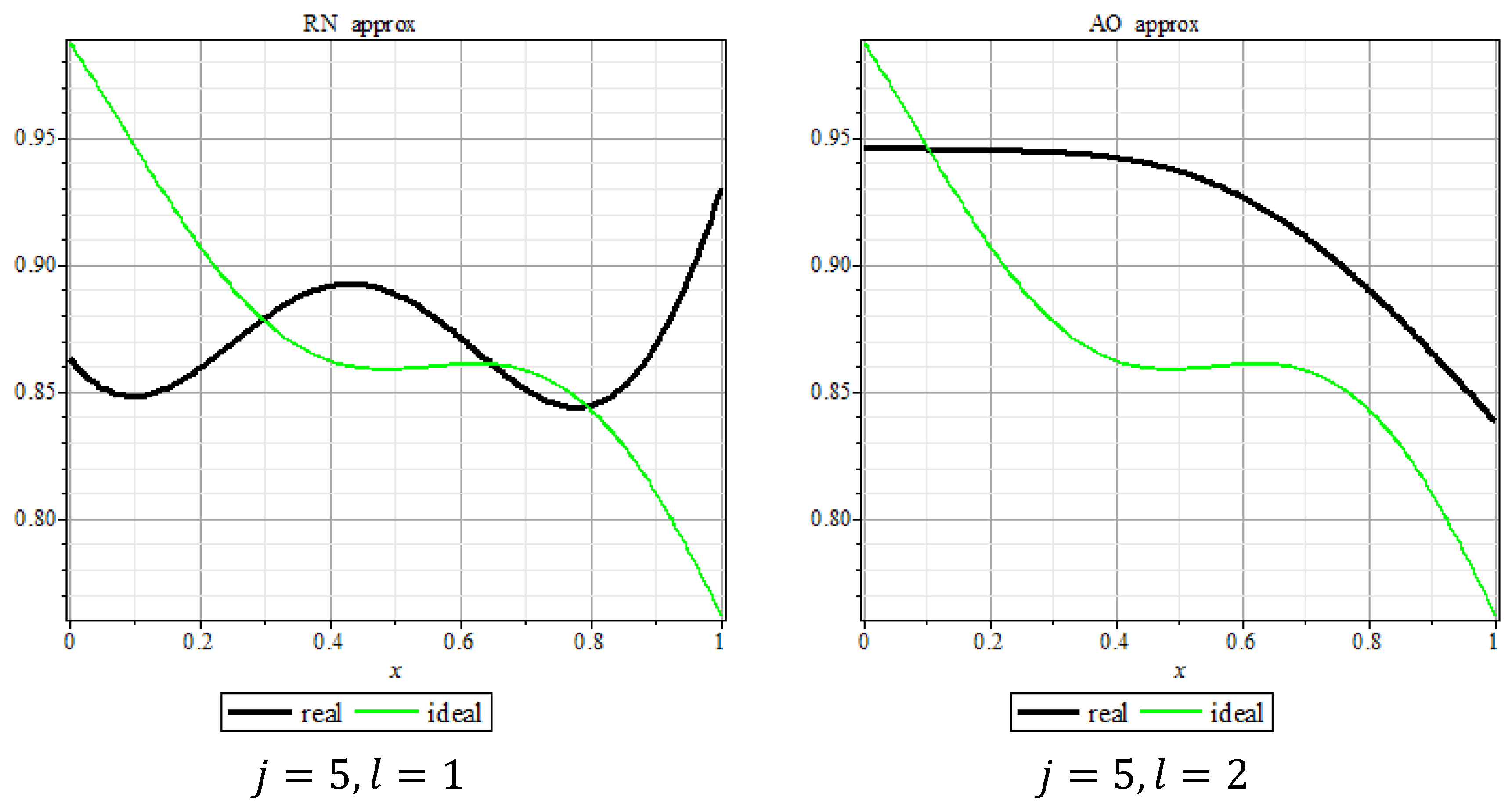
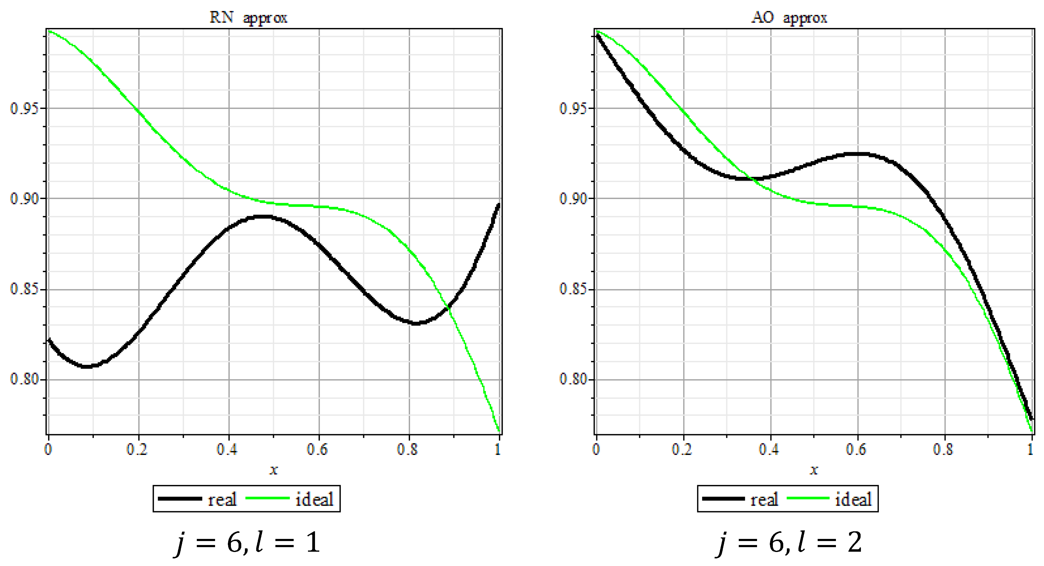
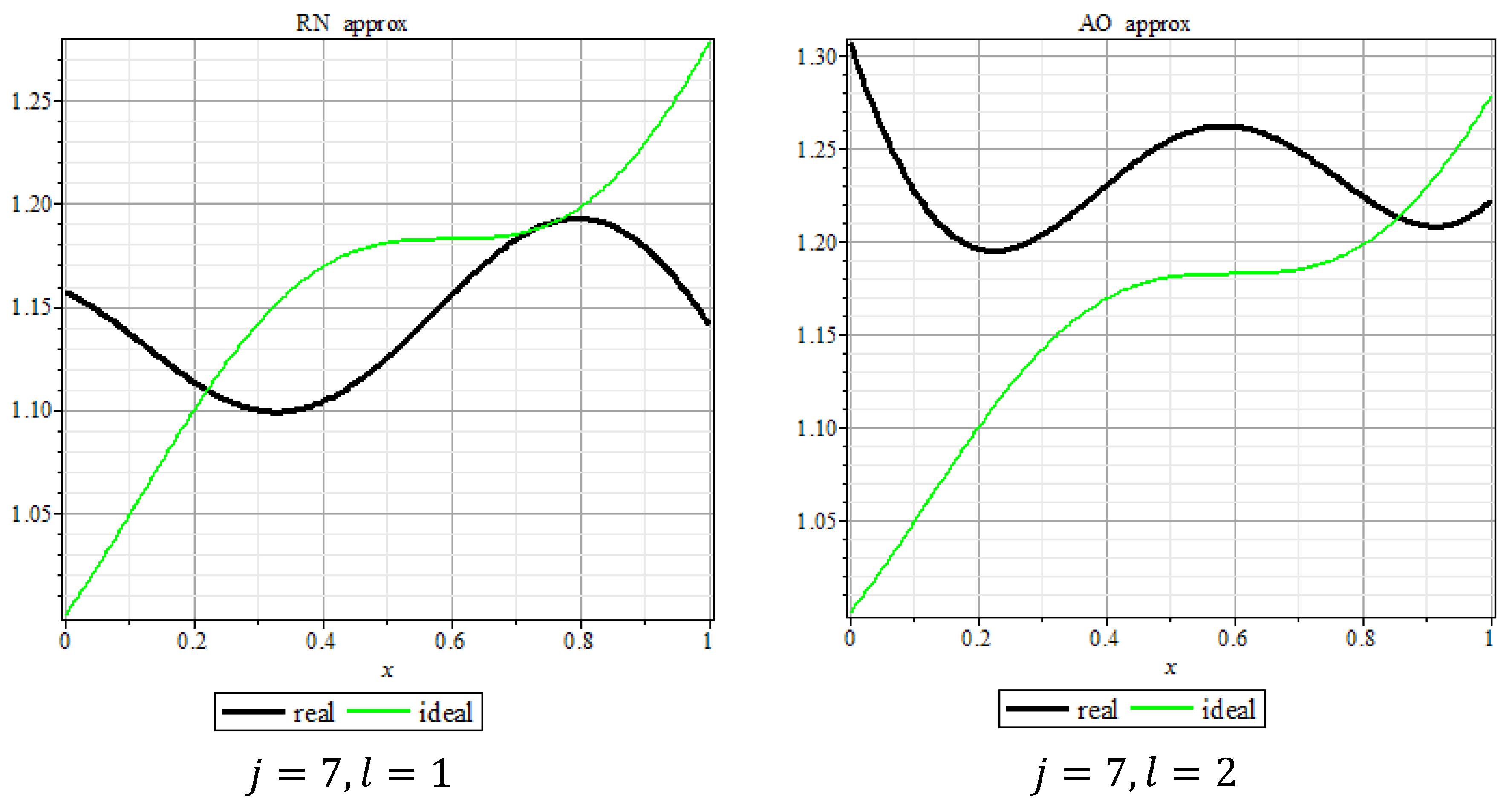
The graphs of approximations of the functions and , with the coefficient values which are given in Table 5, are presented in Figure 3, Figure 4, Figure 5, Figure 6, Figure 7, Figure 8 and Figure 9. The graphs of the approximations of the function are depicted in black, while the approximations of the function are shown in green.

Figure 3.
Approximation of functions and for two athletes according to speed (km/h) at the point of the CIL.
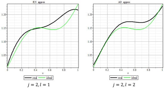
Figure 4.
Approximation of functions for two athletes based on their work capacity (W) at the point of the CIL.
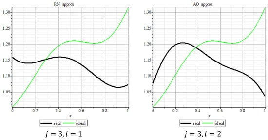
Figure 5.
Approximation of functions for two athletes based on oxygen uptake (1/min, mL/min/kg) at the point of the CIL.

Figure 6.
Approximation of functions for two athletes based on pulmonary ventilation (1/min) at the point of the CIL.

Figure 7.
Approximation of the functions for two athletes based on the resting heart rate (b/min).

Figure 8.
Approximation of the functions for two athletes based on their heart rate (b/min) after the standard physical load.

Figure 9.
Approximation of functions for two athletes based on haemoglobin concentration (g/L).
Visualization of the results provides information about the quality of the athletes’ training management and gives an understanding of the time periods when the maximum discrepancy between the ideal and the real curves can be observed. This allows the coaches to quickly change the athletes’ workouts. To assess the numerical value of this mismatch, the measurement of the difference between the respective functions is required.
It is worth noting that five indicators have a direct relationship with the target, while two indicators, i.e., resting heart rate (5) and heart rate after the standard physical load (6), have the inverse relation with it. By analyzing speed at the point of the CIL (Figure 3), it could be observed that the athlete RN could consistently approach the target (ideal) indicators, although the AO progress was much slower. The tested athletes could not maximally synchronize their efforts (with respect to the above indicator). This can be accounted for by the specific character of their adaptation.
The evaluation of the athletes’ work capacity at the point of the CIL (Figure 4) allows the authors to state that the dynamics of this indicator for the tested athletes was close to the target values, and they achieved their planned peak performance before the beginning of the Olympic Games.
Evaluation of the dynamics of the criteria describing oxygen uptake at the point of the CIL (Figure 5) showed the decreasing trend of VO2max during the testing period and its considerable difference from the target value. This can be accounted for by the specific character of the athletes’ training aimed at increasing the load in the muscles’ area where glycolytic energy is generated. This phenomenon requires further investigation.
When evaluating the variation in the criteria values of pulmonary ventilation at the point of the CIL (Figure 6), a similar trend could be observed as that characteristic of the criteria describing oxygen uptake at the point of the CIL. It can be assumed that the athletes’ aerobic capacity had a tendency to decrease. This can be associated with the striving of athletes to increase their capacity of energy generation in the training period.
Evaluation of the variation of criteria describing the resting heart rate (Figure 7) in a resting position and the heart rate after the application of a standard physical load (Figure 8) showed that the adaptation of the athletes’ circulatory system to training was different. Thus, it was unstable for RN, while AO consistently approached the ideal values of indicators.
The analysis of the variation in hemoglobin concentration of the athletes (Figure 9) has shown that this indicator was difficult to control. In the training process, hemoglobin concentration varied considerably. As a result, the target values could not be achieved before the main competitions.
In the ideal case, when the athlete’s training plan is fully realized, the curves and coincide. In practice, this objective can only be achieved partially; therefore, it is necessary to quantify the difference between the real and the ideal curves.
This difference is a measure of the athletes’ condition. The fact that the differences observed in various time intervals are of various importance is taken into account. The relative importance of the time intervals was determined in the following way. The relative importance of the period prior to measuring was equal to 1, while the importance of other periods was higher, ranging from 2 to 10. The definitions of the time intervals, their relative importance, and the dates and lengths of the intervals (in percent) are given in Table 6.

Table 6.
Relative importance of the time intervals.
Depending on the relative importance of the time intervals and their relative length, the weights were assigned to the normalized time intervals. In this case, . The weights of the time intervals are given in Table 7.

Table 7.
The weights of the time intervals.
It should be emphasized that the fluctuations of the relative importance values in Table 6 were smoothed out. For example, and the intermediate values appeared before , since it was difficult to detect the exact moment of their sudden decrease.
Thus, the difference between the functions and was measured as the weighted sum as follows:
The values calculated for each indicator and both athletes are given in Table 8.

Table 8.
The values for seven indicators and two athletes.
The results provided in Table 8 are summarized as the weighted sums , with the respective criteria weights: (see the data in Table 1). The weighted sums were as follows:
Therefore, . The values have an inverse relationship with the athletic training. The higher these values, the lower the achievement of the goals by the athlete. Then, the values of , describing the results of the athletic training, were calculated as follows:
The higher the value of the indicator K, the higher the level of the fulfillment of the athlete’s training plan. It can be concluded that the results of the second athlete are better than the results obtained by the first athlete. The indicator K is important for the implementation and improvement (optimization) of the athlete’s training plan development.
6. Discussion and Conclusions
The optimization and evaluation of athletic training has become an increasingly important problem for sports scientists, coaches, and athletes [25]. The character of the identification factors of the elite athlete’s condition and their integration into the processes of strategic planning, management, and parameter estimation have not been thoroughly investigated, but they are obviously important. To govern the process of elite athletes’ training, it is required to consider this process both as a whole and in detail. Not all the aspects of the executed cycle can be in compliance. Therefore, the research should not be performed in terms of the standardized compliance management. The OR methods allow us to define the criteria and the limits of their permissible pursuit [14].
The papers considered do not offer a unique view of past research, and the integration they provide is likely to be only fractional. Therefore, real research data are needed. Usually, the research data seem to be more significant than dimensions. They present (1) the constructs and their relational properties and (2) consistency in the measurement of phenomena. The combinations of these dimensions can yield the following results: (1) theoretical plurality and empirical convergence, (2) the dominant paradigm, (3) fragmentation, and (4) the convergent theory and empirical plurality. The integration will require fostering both taxonomic and methodological commensurability among the different sub-fields and contributing disciplines [26]. The method of parameter estimation of the dynamics of the factors presents a viable research approach in this context [27]. It is particularly useful for the investigation of the process cycle, e.g., its long-term effects and results [28]. Interactive data visualization is an evolving approach, providing wide opportunities for managing and decision making in the case of multidimensional decision problems and planning processes.
The proposed methodology of the athletic training visualization makes it easier to identify the advantages and disadvantages of training and shows when (at what stages of training) physical loads (or training methods and techniques) do not match the adaptive capacities of the tested athletes. It also provides new opportunities for streamlining and optimizing the key factors influencing the process by modifying its components. The authors believe that data visualization allows for achieving a better way of informing athletes and coaches about the mistakes and the right choices in the considered training period. According to Xu and Ding [29], visualization allows for identifying the deviations of the indicator values. The automated alarm system, warning about critical deviations of the process components, could help to optimize the process management and prevent hazardous incidents [30].
To the author’s best knowledge, no cases of applying the methodology based on the goal function’s approximation by a linear combination of polynomials and trigonometric functions can be found in the scientific literature on sports management. Meanwhile, this methodology, in conjunction with the least squares method, yields fairly accurate approximation results.
The described methodology (algorithm) has a number of advantages over other similar approaches. The visualization of measurement and target approximation functions enables sports scientists and coaches to perform the following functions:
- to supervise the athletes’ training process,
- to identify undesirable tendencies,
- to correct them immediately (if necessary).
The proposed Formula (4) for measuring the differences between the indicators and the current and target functions enables the researchers to identify the athlete’s condition, as well as showing his/her potential and providing more accurate predictions of sports results.
New opportunities are provided by the proposed method, which:
- Facilitate the understanding and achievement of the goal;
- Make processes clearer to the general public;
- Allow for effective management of the processes.
The provided high-quality, effective alternative solutions to the problem of achieving the final goals of the considered management process give a deeper insight into the effectiveness of a solution, which can support a decision-making process. The principles of the model of the parameter estimation provide visualization capabilities, allowing for evaluating the possibilities to reach the goal, which is the effective management process. This method also allows for predicting the future achievements of athletes.
The proposed model for evaluating the planning of athletic training is used in other sports and can be applied not only to sports practice, but also to the implementation of many various strategies. Moreover, based on the proposed visualization method, an application could be created that would make this method a more widely used technique.
Author Contributions
Conceptualization, S.D.; Data curation, A.K., S.D. and N.K.; Formal analysis, R.D.; Methodology, A.K.; Supervision, S.D.; Visualization, A.K.; Writing—original draft, N.K., R.D.; Writing—review & editing, N.K. and S.D. All authors have read and agreed to the published version of the manuscript.
Funding
This research received no external fundingNo external funding.
Conflicts of Interest
The authors declare no conflict of interest.
References
- Issurin, V.B. Evidence-based prerequisites and precursors of athletic talent: A review. Sports Med. 2017, 47, 1993–2010. [Google Scholar] [CrossRef] [PubMed]
- Jurimae, J. Methods for monitoring training status and their effects on performance in rowing. Int. SportMed J. 2008, 9, 11–21. [Google Scholar]
- Latyshev, M.; Latyshev, S.; Kvasnytsya, O.; Knyazev, A. Performance analysis of freestyle wrestling competitions of the last Olympic cycle. J. Phys. Educ. Sport 2017, 17, 590–594. [Google Scholar]
- Guellich, A.; Seiler, S.; Emrich, E. Training methods and intensity distribution of young world-class rowers. Int. J. Sports Physiol. 2009, 4, 448–460. [Google Scholar]
- Bompa, T.O.; Haff, G. Periodization: Theory and Methodology of Training, 6th ed.; Human Kinetics: Champaign, IL, USA, 2018. [Google Scholar]
- Zatsiorsky, V.M.; Kraemer, W.J. Science and Practice of Strength Training; Human Kinetics: Champaign, IL, USA, 2006. [Google Scholar]
- Halson, S.L. Monitoring training load to understand fatigue in athletes. Sports Med. 2014, 44, 139–147. [Google Scholar] [CrossRef]
- Polak, E.; Kulasa, J.; Vencesbrito, A.; Castro, M.; Fernandes, O. Motion analysis systems as optimization training tools in combat sports and martial arts. Rev. Artes Marciales Asiáticas 2015, 10, 105–123. [Google Scholar] [CrossRef]
- Fister, I.; Rauter, S.; Yang, X.-S.; Ljubic, K. Planning the sports training sessions with the bat algorithm. Neurocomputing 2015, 149, 993–1002. [Google Scholar] [CrossRef]
- Dadelo, S.; Turskis, Z.; Zavadskas, E.K.; Kačerauskas, T.; Dadelienė, R. Is the Evaluation of the Students’ Values Possible? An Integrated Approach to Determining the Weights of Students’ Personal Goals Using Multiple-Criteria Methods. Eurasia J. Math. Sci. Technol. 2016, 12, 2771–2781. [Google Scholar] [CrossRef]
- Armstrong, K.J.; Weidner, T.G.; Walker, S.E. Athletic training approved clinical instructors’ reports of real-time opportunities for evaluating clinical proficiencies. J. Athl. Train. 2009, 44, 630–638. [Google Scholar] [CrossRef]
- Li, F.; Zhu, Q.; Chen, Z.; Xue, H.A. A balanced data envelopment analysis cross-efficiency evaluation approach. Expert Syst. Appl. 2018, 106, 154–168. [Google Scholar] [CrossRef]
- Karsu, Ö.; Morton, A. Incorporating balance concerns in resource allocation decisions: A bi-criteria modelling approach. Omega 2014, 44, 70–82. [Google Scholar] [CrossRef][Green Version]
- Reefke, H.; Sundaram, D. Key themes and research opportunities in sustainable supply chain management—Identification and evaluation. Omega 2017, 66, 195–211. [Google Scholar] [CrossRef]
- Recalde, D.; Torres, R.; Vaca, P. Scheduling the professional Ecuadorian football league by integer programming. Comput. Oper. Res. 2013, 40, 2478–2484. [Google Scholar] [CrossRef]
- Dadelo, S.; Turskis, Z.; Zavadskas, E.K.; Dadelienė, R. Multi-criteria assessment and ranking system of sport team formation based on objective-measured values of criteria set. Expert. Syst. Appl. 2014, 41, 6106–6113. [Google Scholar] [CrossRef]
- Jones, C. Visualization and Optimization. J. Oper. Res. Soc. 1997, 48, 964. [Google Scholar] [CrossRef]
- Laengle, S.; Merigó, M.M.; Miranda, J.; Słowiński, R.; Bomze, I.; Borgonovo, E.; Dyson, R.G.; Oliveira, J.F.; Teunter, R. Forty years of the European Journal of Operational Research: A bibliometric overview. Eur. J. Oper. Res. 2017, 262, 803–816. [Google Scholar] [CrossRef]
- Moritz, D.; Fisher, D.; Ding, B.; Wang, C. Trust, but verify optimistic visualizations of approximate queries for exploring big data. In Proceedings of the 2017 CHI Conference on Human Factors in Computing Systems, CHI’17, Denver, CO, USA, 6–11 May 2017; pp. 2904–2915. [Google Scholar]
- Balčiūnas, E. Didelio Meistriškumo Baidarininkų Rengimas 200 ir 500 m Nuotoliams: Monografija/Training of Elite Kayakers for Distances of 200 and 500 m: The Monograph; Lietuvos edukologijos universiteto leidykla: Lithuania, Vilnius, 2016. (In Lithuania) [Google Scholar]
- Norton, K.; Olds, T. Antropometrica; University of New South Wales Press: Sydney, Australia, 1996. [Google Scholar]
- Thodens, J.S. Testing Aerobic Power. Physiological Testing of the High-Performance Athlete; Human Kinetics: Champaign, IL, USA, 1991. [Google Scholar]
- Legendre, A.-M. Nouvelles Méthodes pour la Détermination des Orbites des Comètes [New Methods for the Determination of the Orbits of Comets]; F. Didot: Paris, France, 1805. (In French) [Google Scholar]
- Strang, G. Linear Algebra and Its Applications, 4th ed.; Cengage Learning: Boston, MA, USA, 2006. [Google Scholar]
- Spotts, J.D. Global politics and the Olympic Games: Separating the two oldest games in history. Dickinson J. Int. Law 1994, 13, 103–122. [Google Scholar]
- Durand, R.; Grant, R.M.; Madsen, T.L. The expanding domain of strategic management research and the quest for integration. Strateg. Manag. J. 2017, 38, 4–16. [Google Scholar] [CrossRef]
- Krylovas, A.; Dadeliene, R.; Kosareva, N.; Dadelo, S. Comparative evaluation and ranking of the European countries based on the interdependence between human development and internal security indicators. Mathematics 2019, 7, 293. [Google Scholar] [CrossRef]
- Sivarajah, U.; Kamal, M.M.; Irani, Z.; Weerakkody, V. Critical analysis of Big Data challenges and analytical methods. J. Bus. Res. 2017, 70, 263–286. [Google Scholar] [CrossRef]
- Xu, L.; Ding, F. Recursive least squares and multi-innovation stochastic gradient parameter estimation methods for signal modelling. Circuits Syst. Signal Process. 2017, 36, 1735–1753. [Google Scholar] [CrossRef]
- Krylovas, A.; Dadelo, S.; Kosareva, N.; Zavadskas, E.K. Entropy-KEMIRA approach for MCDM problem solution in human resources selection task. Int. J. Inf. Technol. Decis. Mak. 2017, 16, 1183–1209. [Google Scholar] [CrossRef]
© 2020 by the authors. Licensee MDPI, Basel, Switzerland. This article is an open access article distributed under the terms and conditions of the Creative Commons Attribution (CC BY) license (http://creativecommons.org/licenses/by/4.0/).

