Advanced Mathematical Business Strategy Formulation Design


School of Applied Sciences, Macao Polytechnic Institute, Macao
†
Current address: R. de Luis Gonzaga Gomes, Macao, SAR.
Mathematics 2020, 8(10), 1642; https://doi.org/10.3390/math8101642
Submission received: 17 August 2020
/
Revised: 15 September 2020
/
Accepted: 15 September 2020
/
Published: 23 September 2020
(This article belongs to the Special Issue Mathematical Analysis in Economics and Management)
Abstract
:This paper deals with the explicit design of strategy formulations to make the best strategic choices from a conventional matrix form of representing strategic choices. The explicit strategy formulation is an analytical model that is targeted to provide a mathematical strategy framework to find the best moment for strategy shifting to prepare rapid market changes. This theoretical model could be adapted into practically any strategic decision making situation when a strategic formulation is described as a matrix form with quantitative measured decision parameters. Analytically tractable results are obtained by using the fluctuation theory and these results are able to predict the best moments for changing strategies in a matrix form. This research can help strategy decision makers who want to find the optimal moments of shifting present strategies.
Keywords:
strategy; strategy formulation; fluctuation theory; first exceed model; BCG growth-share matrix; business level strategyMSC:
60G40; 60G55; 62C25; 60K99; 90B50; 90B60; 91B06; 91B70
1. Introduction
A strategy is a set of actions that contains the execution of core competencies and the collection of competitive advantages. The determination of long-run goals, the establishment of a series of actions, and the allocation of resources are handled to carry out strategic goals. Hence, companies could make choices among competing alternatives for the pathway to pursue strategic competitiveness by choosing proper strategies. Strategic management consists of operating the full set of commitments, decisions, and actions for gaining break-even returns by achieving strategic competitiveness [1,2,3]. Strategy formulation is a particular process of choosing the most appropriate strategic actions for realizing objectives and for achieving the visions of a company [4]. Formulation results provide a blueprint of strategic actions to achieve the goals of a company. A strategy formulation forces a company to find the moments of environment changes and to be ready for shifting strategies [5]. A conventional strategic formulation includes defining a corporate mission, specifying achievable objectives, developing strategies, and setting policy guidelines [3]. It is also based on the sources of decision parameters that could develop visions and missions of a company by formulating one or more strategies with available information [1].
As a part of a strategic formulation, many strategic decision making matrices have been developed, including the issues priority matrix by Lederman [6], the business level strategy by Porter [7], the strategy clock by Bowman [8], the product and market expansion grid by Ansoff [9], and the business portfolio matrix by the Boston Consulting Group [10]. In addition, the matrix form could also be applied to outsourcing strategy [3], value-creation diversification strategies [1], and performance matrices [11].
The main contribution of this paper is providing a general framework for formulating a strategy that is explicitly designed and mathematically proven; a theory to determine the explicit probability of the strategy shifting is also included. This mathematical model explicitly identifies the best moment of shifting strategic choices and the analytical form can even count one step prior to pass the thresholds of strategic decision parameters. The fluctuation theory is one of the powerful mathematical tools in stochastic modeling and the first exceed model is a variation of conventional fluctuation models [12,13].
In a fluctuation model [12,13], the multi-compound renewal process evolves until either of the components hits (i.e., reaches or exceeds) their assigned levels for the first moment and the associated random variables, which include the first passage time, the first passage level, and the termination index. The first exceed level theory in the fluctuation model has been applied in various applications, including antagonistic games [14,15,16], stochastic defense systems [17], blockchain governance games [18,19], and versatile stochastic duel games [20,21]. Analytically solving probability distributions by using a variation of a fluctuation model [13,14,15] is one of core contributions of this paper.
The paper is organized as follows: Section 2 provides a literature review of various strategic decision matrices. Various strategic formulation methods are introduced to show how the formulations are intuitively described by a simple matrix form. The stochastic model using first exceed level theory is fully mathematically analyzed in Section 3. The closed formula to find the optimal moments of the strategy shifting is analytically proven and the explicit solutions are obtained by analytically solving a special process rather than from quantitative data. The initial conditions for adapting this mathematical model into actual strategy formulations are also mentioned in this section. The actual adaptation of this analytical model into a BGC growth-share matrix is demonstrated with the scale changes of its decision parameters [10] in Section 4. Users can find the method of implementing this new mathematical model into one of the well-known strategic formulation matrices. Finally, conclusions are presented in Section 5.
2. Literature Review
A strategy formulation helps a company prepare the moment of shifting strategies. The 10 most popular strategy formulation tools are introduced in this literature review. As mentioned in the previous section, strategic formulation tools include the business level strategy by Porter [7], the product-market matrix by Ansoff [9], and the growth-share matrix by the Boston Consulting Group [22,23]. The purpose of this section is to show how a simple matrix form could be adapted into various strategic formulations intuitively. It is noted that actual applications for using strategic formulations will not be covered in this section.
Strategic group mapping: Strategic groups are groups of whose team members are gathered according to similar strategic characteristics, following similar strategies within an industry or a sector [2]. Strategic group matrix maps are based on the R&D intensities and export focuses that distinguish between strategic groups. This simple strategy formulation could describe strategic groups as a matrix form that is categorized based on R&D intensity and export focus. A user could choose a proper strategy based on these two decision parameters [2] (see Figure 1).
Stakeholder priority matrix: This is another matrix form that describes stakeholders based on the interests of shareholders and their involvement power [24]. As shown in Figure 2, each stakeholder group can be shown graphically based on its level of interest (from low to high) and on its relative power (from low to high). Although managers could take some stakeholders for granted, it may lead to serious problems later because of a conflict of interest [1].
Stakeholder mapping [2] formulates different strategies based on the same decision parameters as the stakeholder priority matrix. As mentioned in the previous section, this matrix is targeted more toward how to deal with stakeholders (see Figure 3).
Issues priority matrix: This is a strategic formulation used to identify and analyze developments in the external environment [3,6]. The issues priority matrix is applied to help managers to decide which environmental trends should be merely scanned (i.e., low priority) and which should be monitored as strategic factors (i.e., high priority). The decision parameters are the probable impacts and the chances of occurrences (see Figure 4).
The Value-creation diversification matrix is a matrix form of a corporate-level strategy that specifies actions [1]. Corporate-level strategies help firms select new strategic positions and the matrix specifies actions of a company to gain a competitive advantage by selecting a proper strategy. Operational relatedness and corporate relatedness are the decision parameters used to determine a best strategy. The decision parameter of the vertical dimension is an opportunity to share operational activities between businesses while the horizontal dimension suggests an opportunity for transferring corporate-level core competencies (see Figure 5).
The business level strategy [1,3,7,25,26] focuses on improving the competitive position of a product or a service within a specific industry. A study showed that a business unit efficiency doubled the impact on overall company performance relative to both corporation and industry changes [3]. Based on competitive advantages and scopes, a company selects one of four business-level strategies to establish and defend their desired strategic position against competitors: cost leadership, differentiation, focused cost, and focused differentiation (see Figure 6).
The strategy clock, which was developed by Bowman [8], is a model that explores options for strategic positioning. It indicates how a product should be positioned to give the most competitive position in the market [27]. This strategy formulation is used to illustrate a variety of options of positioning a product based on the two dimensions of price and perceived value [2]. The original strategy clock looks like a clock but it could also be presented in matrix form (see Figure 7).
The GE-McKinsey nine-box matrix is another matrix form of a strategy formulation that describes a systematic approach to determine the best position to invest cash [28]. A company could analyze its status by using the two decision parameters (the attractiveness of the relevant industry and the competitive strength within that industry) that determine whether it is going to do well or not in the future [28]. This three-by-three matrix was developed by McKinsey to consult the complex portfolio of unrelated GE products in 1970s [29]. The candidate strategies are mainly invest (or grow), leave (or hold) and drop (or divest), which are determined based on the decision parameters (see Figure 8).
The Boston Consulting Group (BCG) product portfolio matrix (also known as a growth-share matrix) is given to the various segments within their mix of businesses [1]. This portfolio matrix has been designed and developed by the BCG since the 1970s [22,23]. The matrix form has been used to build a long-term strategic plan and business growth opportunities by reviewing a company’s portfolio of products to decide where to invest and how to develop products. The decision parameters of the growth-share matrix are the rate of market growth and the market share. The matrix plots four strategies in a two-by-two matrix form as shown in Figure 9. One of the strategic choices mentioned in Table 1 is determined based on the decision parameters [23].
It is noted that a BCG growth-share matrix contains a quantitative scale of each decision parameter [10]. Therefore, the newly proposed analytical model in the paper could be easily adapted into this matrix form. As previously mentioned, the actual implementation of the mathematical model into a BCG growth-share matrix is provided in Section 4.
Product-market matrix (also known as the Ansoff matrix): Strategic marketing planning should find opportunities to grow revenue for a business through developing new products. The product-market matrix is one of most widely used strategic formulation tools in marketing. This matrix is mainly used to evaluate opportunities for companies to increase their sales through showing alternative combinations for new markets against products and services offering four strategies, as shown in Figure 10 [9].
3. The Explicit Mathematical Model
3.1. Preliminaries
Let be the probability space of independent -subalgebras, and be the monotone nondecreasing random values of two strategic selection factors, indicating that business growth and market competitiveness are continuously increased when the time passes under idle conditions (i.e., no competition in the market). Suppose:
where -measurable and -measurable are marked Poisson processes ( is a point mass at a) with respective intensities and and point-independent marking. From (1) and (2), the random values and are the nondecreasing random impacts of strategic decisions that are related to strategy transitions. In the BGC growth-share matrix, these random values, and , represent the rate of competitive position factor and the business growth rate factor respectively (see Section 4). The status of each decision making parameter is observed at random times in accordance with the point process [13,16,19]:
which is assumed to be a delayed renewal process. A delayed renewal point process is the same as an ordinary renewal point process, except that the first point mass is allowed to have a different one. The formula (3) is the formal form of a delayed renewal point process with a point mass at the moment a and it becomes the sum of point masses. It is noted that point masses at are inter-arrival times between the interval . Let:
be the nondecreasing random measures for strategic impacts of two decision parameters embedded over . With respective increments, we have:
and
The observation process upon could be formalized as:
where
With position-dependent marking, and become dependent with the following notation:
and
where
By using the double expectation,
The functional is defined on the space of all analytic functions at 0 and has the following properties:
- (i)
- is a linear functional with fixed points at constant functions;
- (ii)
Theorem 1.
The functional of the process from (18) satisfies the following expression:
where
Proof.
We find the explicit formula of the joint function from (18) as follows:
and, by applying the operator , we arrive at:
and, from the previous research [12,13],
where
From (33),
where
Similarly, from (34),
where
Then, we have
where
or
From (21), we have:
therefore,
□
From (13)–(18) and (24), we can find the probability generating functions (PGFs) of the exit indexes and as follows:
3.2. General Framework for Mathematical Strategy Formulation
Recalling from the previous section, the matrix form is a typical way to describe a set of strategic choices based on the decision parameters (i.e., the category of the strategy input) in the strategy formulation. Most strategy formulations could be described by the matrix. This section deals with the conventional two-by-two matrix form to combine the fluctuation theory for determining the proper strategic decision making. The stakeholder mapping [2] in Figure 3, the product-market matrix in Figure 10, the business level strategy in Figure 6, and the BCG product portfolio in Figure 9 are intuitively described by a two-by-two matrix form.
A conventional two-by-two matrix provides four strategic choices (I–IV), and an optimal strategic choice depends on a present or future position of a company (see Figure 11). Let us assume that decision parameters are quantitative. From (16) and (17), the thresholds are equivalent with m and n respectively. Strategy (I) becomes the best choice, where , , and strategy (II) are the best choice where , . Formally speaking, a best strategic choice could be chosen as follows:
where is the best strategy function (BSF) of a BGC matrix and the moment of selecting a strategic choice becomes critical. The first exceed model could analytically find the moment in which to take a strategic action. Generally, the moment of shifting the strategy is the time when the decision parameters pass their thresholds , which could be determined analytically from (16) and (17). It is noted that a strategic choice could even be shifted before passing the strategic thresholds, which are and instead of the first exceed moments and .
3.3. Strategy Shifts under Memoryless Observation
This section assumes that the observation process has the memoryless property which might be considered as a special case. However, the memoryless property is practical for an actual implementation onto a decision making system because this property makes the system not contain any past information. It also implies that the observation process dose not have any dependence with strategic decision parameters. Recalling from (19), the operator is defined as follows:
then
where are a sequence, with the inverse (21) and
and
The marginal mean of and is the moment of the strategy chances and it could be straightforward once the exit index is found. Each exit index of the decision parameters A and B could be found from Lemmas 1 and 2 (see Appendix A and Appendix B):
Lemma 1.
The probability generating function (PGF) of the exit index for the decision parameter A under a memoryless observation process could found as follows:
Lemma 2.
The PGF of the exit index for the decision parameter B under a memoryless observation process could be:
where
From (59) and (60), we have:
3.4. Useful Tips for Theoretical Modeling
Since we are dealing with a mathematical approach, it is impossible to apply a theoretical model into a practical implementation without adjustments. Although all strategy formulations discussed in the literature review are described as a matrix form, not all of them have quantitative decision parameters. It is noted that all decision parameters should be quantitative and the thresholds should be measurable to be applied into an analytical model. Additionally, the scale of decision parameters might be modified for sustaining the linearity of the decision parameter values. In this newly proposed mathematical strategy formulation model, it should be assumed that the process for each decision parameter is the Poisson compound process and this is the most mandatory condition that makes the mathematical model analytically solvable. Instead of the Poisson process, a generally distributed random process of each decision parameter might be considered when the related data are possibly obtained. Similarly, a numerical approach could be considered instead of an analytical approach if it is feasible to collect suitable real data in a certain way. Lastly, the observation process might have memoryless properties, which implies that the observation process does not contain any past information.
4. BCG Growth-Share Matrix Reloaded
The BCG growth-share matrix contains the quantitative scale of each decision parameter (see Figure 12) and is one of the intuitive ways to portray a company portfolio strategy [10]. According to Hedley, the separating areas of high and low relative competitive position are set at 1.5 times [10]. When the business growth rate is more than 10 percent, a product has relative strengths of this magnitude to ensure that the dominant position needs to be the (III) or the (IV). On the other hand, a product that has a relative competitive position could be either (I) or (II). Each status will have a different strategy and the strategy should be shifted when the status is changed.
In the BGC growth-share matrix model, represents the transformed random value from the a market share of a product (or a company) at the j-th epoch, and represents a growth rate (%) of a market at the k-th epoch. Both are assumed to be monotone nondecreasing until a strategy is shifted. The scale of the BCG matrix should be modified to adapt the mathematical model and the scale of the relative competitive position is mapped as follows:
The market share is transformed into the relative competitive ratio with the revised scale (i.e., the x-axis in Figure 12) and the modified mapping scale could be as shown in Figure 13.
From (36) and (69), the best strategy for the BCG matrix is determined as follows:
and the optimal moments to shift the strategies and are determined from (67) and (68).
5. Conclusions
The main contribution of this paper is establishing a theoretical framework for strategy formulations by providing the explicit forms from a conventional strategy formulation matrix. The mathematical analysis that includes the explicit functionals for finding the optimal moments of the strategy shifts and strategy executions was fully deployed in this paper. This analytical approach supports the theoretical background of the strategic choice to make the best decisions from advanced mathematical strategy formulations. Additionally, this newly proposed analytical model was applied on the BCG growth-share matrix to demonstrate the actual implementation of the model. This research shall be helpful for whoever is looking for scientific strategy executions in real business matters.
Funding
This research received no external funding.
Acknowledgments
Special thanks to the guest editor, Yi-Hsien Wang, who guided the author to submit the paper to the proper journal; the author is also thankful to the referees whose comments were very constructive. There are no available data to be stated.
Conflicts of Interest
The author declares no conflict of interest.
Appendix A. Proof of Lemma 1
The probability generating function of could be straightforward once the exit index is found. The exit index could be found from (18), (23), (24) and (30):
where
Proof of Lemma 1.
The probability generating function (PGF) of the exit index for the decision parameter A could be found as follows:
From (43),
From (A2),
and
where
From (A6) and (A7),
Therefore,
where
From (A1) and (A11)–(A12),
□
Appendix B. Proof of Lemma 2
Proof of Lemma 2.
The probability generating function of is found as follows:
where
From (48),
where
Therefore,
□
References
- Hitt, M.A.; Ireland, R.D. Concepts Strategic Management: Competitiveness & Globalization, 9th ed.; South-Western Cengage Learning: Mason, OH, USA, 2011. [Google Scholar]
- Johnson, G.; Whittington, R.; Scholes, K.; Angwin, D.; Regner, P. Exploring Strategy Text and Cases, 11th ed.; Pearson: Harlow, UK, 2017. [Google Scholar]
- Wheelen, T.L.; Hunger, J.D. Strategic Management and Business Policy, 13th ed.; Pearson: Upper Saddle River, NJ, USA, 2012. [Google Scholar]
- Juneja, P. Steps in Strategy Formulation Process. 2019. Available online: https://www.managementstudyguide.com/strategy-formulation-process.htm (accessed on 1 May 2019).
- Salor Foundation, Strategy Formulation. 2019. Available online: https://resources.saylor.org/wwwresources/archived/site/wp-content/uploads/2013/09/Saylor.orgs-Strategy-Formulation.pdf (accessed on 1 May 2019).
- Lederman, L.L. Foresight Activities in the U.S.A.: Time for a Re-Assessment? Long Range Plan. 1984, 17, 41–50. [Google Scholar] [CrossRef]
- Porter, M.E. From Competitive Advantage to Corporate Strategy. Readings in Strategic Management; Palgrave: London, UK, 1989; pp. 234–255. [Google Scholar]
- Bowman, C.; Faulkner, D. Competitive and Corporate Strategy; Irwin: London, UK, 1997. [Google Scholar]
- Ansoff, I. Strategies for Diversification. Harv. Bus. Rev. 1957, 35, 113–124. [Google Scholar]
- Hedley, B. Strategy and the Business Portfolio. Long Range Plan. 1977, 10, 9–15. [Google Scholar] [CrossRef]
- Crossan, M. Strategic Analysis and Action; W09374-PDF-ENG; Harvard Business Publishing: Brighton, MA, 2011; 43p. [Google Scholar]
- Dshalalow, J.H. First excess level process. In Advances in Queueing; CRC Press: Boca Raton, FL, USA, 1995; pp. 244–261. [Google Scholar]
- Dshalalow, J.H.; Ke, H.-J. Layers of noncooperative games. Nonlinear Anal. 2009, 71, 283–291. [Google Scholar] [CrossRef]
- Dshalalow, J.H. Random Walk Analysis in Antagonistic Stochastic Games. Stoch. Anal. Appl. 2008, 26, 738–783. [Google Scholar] [CrossRef]
- Dshalalow, J.H.; Huang, W.; Ke, H.J.; Treerattrakoon, A. On Antagonistic Game with a Constant Initial Condition Marginal Functionals and Probability Distributions. Nonlinear Dyn. Syst. Theory 2016, 16, 268–275. [Google Scholar]
- Dshalalow, J.H.; Iwezulu, K.; White, R.T. Discrete Operational Calculus in Delayed Stochastic Games. Neural Parallel Sci. Comput. 2016, 24, 55–64. [Google Scholar]
- Kim, S.-K. Enhanced Design of Stochastic Defense System with Mixed Game Strategies. In Game Theory for Networking Applications; Springer: Berlin, Germany, 2018; pp. 107–117. [Google Scholar]
- Kim, S.-K. Blockchain Governance Game. Comput. Indu. Eng. 2019, 136, 373–380. [Google Scholar] [CrossRef] [Green Version]
- Kim, S.-K. Strategic Alliance for Blockchain Governance Game. Probab. Eng. Informational Sci. 2020. [Google Scholar] [CrossRef]
- Kim, S.-K. A Versatile Stochastic Duel Game. Mathematics 2020, 8, 678. [Google Scholar] [CrossRef]
- Kim, S.-K. Antagonistic One-To-N Stochastic Duel Game. Mathematics 2020, 8, 1114. [Google Scholar] [CrossRef]
- Hanlon, A. How to Use the BCG Matrix Model. 2019. Available online: https://www.smartinsights.com/marketing-planning/marketing-models/use-bcg-matrix/ (accessed on 1 May 2019).
- Kenton, W. BCG Growth-Share Matrix. 2019. Available online: https://www.investopedia.com/terms/b/bcg.asp (accessed on 1 May 2019).
- Anderson, C. Values-Based Management. Acad. Mgt. Execc. 1997, 11, 25–46. [Google Scholar] [CrossRef]
- Weissenberger-Eibl, M.A.; Almeida, A.; Seus, F. A Systems Thinking Approach to Corporate Strategy Development. Systems 2019, 7, 16. [Google Scholar] [CrossRef] [Green Version]
- Kumar, M.; Tsolakis, N.; Agarwal, A.; Srai, J.S. Developing distributed manufacturing strategies from the perspective of a product-process matrix. Int. J. Prod. Econ. 2020, 219, 1–17. [Google Scholar] [CrossRef]
- Riley, J. Bowman’s Strategic Clock. 2016. Available online: https://www.tutor2u.net/business/reference/strategic-positioning-bowmans-strategy-clock (accessed on 1 May 2019).
- McKinsey & Company. McKinsey Quarterly. 2008. Available online: https://www.mckinsey.com/business-functions/strategy-and-corporate-finance/our-insights/enduring-ideas-the-ge-and-mckinsey-nine-box-matrix (accessed on 1 May 2019).
- Enalls, T. GE McKinsey Matrix: How to Apply It to Your Business. 2017. Available online: http://ideagenius.com/ge-mckinsey-matrix-apply-business/ (accessed on 1 May 2019).
Figure 1.
Strategic group mapping [2].
Figure 1.
Strategic group mapping [2].

Figure 2.
Stakeholder priority matrix [2].
Figure 2.
Stakeholder priority matrix [2].

Figure 3.
Stakeholder mapping [2].
Figure 3.
Stakeholder mapping [2].

Figure 4.
Issues priority matrix adapted from Lederman [6].
Figure 4.
Issues priority matrix adapted from Lederman [6].

Figure 5.
Value-creation diversification matrix [1].
Figure 5.
Value-creation diversification matrix [1].

Figure 6.
Business level strategy matrix adapted from Porter [7].
Figure 6.
Business level strategy matrix adapted from Porter [7].
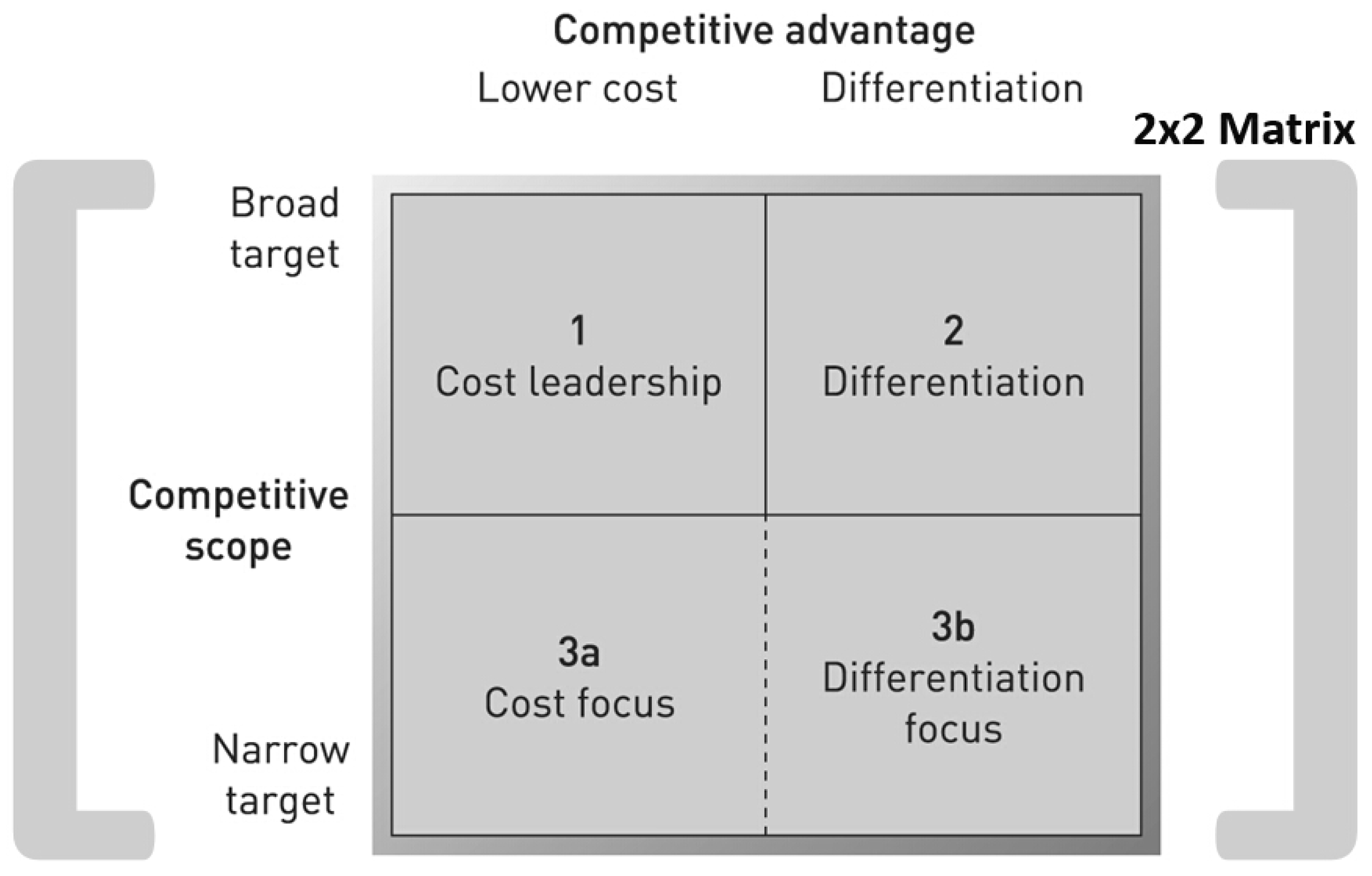
Figure 7.
Strategy clock strategy matrix [27].
Figure 7.
Strategy clock strategy matrix [27].

Figure 8.
GE-McKinsey nine-box matrix [29].
Figure 8.
GE-McKinsey nine-box matrix [29].

Figure 9.
Boston Consulting Group (BCG) product portfolio matrix [23].
Figure 9.
Boston Consulting Group (BCG) product portfolio matrix [23].

Figure 10.
Product-market matrix, adapted from Ansoff [9].
Figure 10.
Product-market matrix, adapted from Ansoff [9].

Figure 11.
Conventional 2 × 2 strategy matrix.

Figure 12.
BCG growth-share matrix [10].
Figure 12.
BCG growth-share matrix [10].

Figure 13.
Scale modification of the BCG matrix.


Table 1.
Strategic choices based on the BGC matrix.
| I | Dogs | The usual marketing advice here is to aim to remove any dogs from the product portfolio as they are a drain on resources. |
| II | Cows | The simple rule here is to “Milk these products as much as possible without killing the cow”. Often used for mature, well-established products. |
| III | Stars | The market leaders, though they require ongoing investment to sustain. They generate more ROI (return-of-investment) than other product categories. |
| IV | Question Marks | These products often require significant investment to push them into the star quadrant. |
© 2020 by the author. Licensee MDPI, Basel, Switzerland. This article is an open access article distributed under the terms and conditions of the Creative Commons Attribution (CC BY) license (http://creativecommons.org/licenses/by/4.0/).
Share and Cite
MDPI and ACS Style
Kim, S.-K. Advanced Mathematical Business Strategy Formulation Design. Mathematics 2020, 8, 1642. https://doi.org/10.3390/math8101642
AMA Style
Kim S-K. Advanced Mathematical Business Strategy Formulation Design. Mathematics. 2020; 8(10):1642. https://doi.org/10.3390/math8101642
Chicago/Turabian StyleKim, Song-Kyoo (Amang). 2020. "Advanced Mathematical Business Strategy Formulation Design" Mathematics 8, no. 10: 1642. https://doi.org/10.3390/math8101642
Note that from the first issue of 2016, this journal uses article numbers instead of page numbers. See further details here.