Abstract
In recent years, deep learning models have been used successfully in almost every field including both industry and academia, especially for computer vision tasks. However, these models are huge in size, with millions (and billions) of parameters, and thus cannot be deployed on the systems and devices with limited resources (e.g., embedded systems and mobile phones). To tackle this, several techniques on model compression and acceleration have been proposed. As a representative type of them, knowledge distillation suggests a way to effectively learn a small student model from large teacher model(s). It has attracted increasing attention since it showed its promising performance. In the work, we propose an ensemble model that combines feature-based, response-based, and relation-based lightweight knowledge distillation models for simple image classification tasks. In our knowledge distillation framework, we use ResNet−20 as a student network and ResNet−110 as a teacher network. Experimental results demonstrate that our proposed ensemble model outperforms other knowledge distillation models as well as the large teacher model for image classification tasks, with less computational power than the teacher model.
1. Introduction
During the last few years, deep learning models have been used successfully in numerous industrial and academic fields, including computer vision [1,2], reinforcement learning [3], and natural language processing [4]. However, training data is not sufficient to effectively train deep learning models in many applications. Therefore, it is necessary to develop compact networks that generalize well without requiring large-scale datasets. Furthermore, most deep learning models are computationally expensive to run on resource-limited devices such as mobile phones and embedded devices.
To overcome these limitations, several model compression techniques (e.g., low-rank factorization [5,6,7], parameter sharing and pruning [8,9,10,11,12,13,14,15,16,17,18,19], and transferred/compact convolutional filters [20,21,22,23,24,25]) have been proposed for reducing the size of the models while still providing similar performance. One of the most effective techniques is knowledge distillation in a teacher-student setting, where a larger pretrained network (teacher network) produces output probabilities which are then used to train a smaller compact network (student network). Hence, it provides greater architectural flexibility since the structural differences between the teacher and student are allowed. Additionally, instead of training with one-hot-encoded labels where the classes are mutually exclusive, using the relative probabilities of secondary classes or relational information between data examples provides more information about the similarities of the samples, which is the core part of the knowledge distillation. Despite its simplicity, knowledge distillation shows promising results in various fields including image classification.
Generally, knowledge distillation methods can be divided into (1) response-based (2) feature-based, and (3) relation-based distillation methods depending on which forms of knowledge is transferred into the student network. In the response-based distillation method, the neural response of the last output layer of the teacher network is used. For instance, Ba and Caruana [26] used logits as knowledge. Hinton et al. [27] adopted the category distribution (soft target) as the distilled knowledge. In the feature-based distillation method, the output of the intermediate (i.e., feature maps) and last layers are all utilized as knowledge for supervising the training of the student model. For instance, FitNet [28] uses intermediate feature maps of the teacher network to improve performance. The work in [29] proposed Attention Transfer (AT) to transfer the attention maps which represent the relative importance of layer activations. In the relation-based distillation method, the relationships between data samples and different layers are further utilized in relation-based knowledge. For instance, Park et al. proposed Relational Knowledge Distillation (RKD) [30] to transfer relations of data examples based on distance-wise and angle-wise distillation losses which measure structural differences in relations. Peng et al. [31] proposed a method based on correlation congruence (CC), in which the distilled knowledge contains information of instances and the correlations between two instances.
In this work, we propose an ensemble model that combines three lightweight models learned by three different knowledge distillation strategies (feature-based, response-based, and relation-based) on CIFAR-10 and CIFAR-100 datasets which are widely used as the benchmarks for the image classification task. For knowledge distillation, we adopt ResNet-20 as a lightweight student network, containing only 0.27 million parameters, and ResNet-110 as a teacher network, containing 1.7 million parameters for knowledge distillation.
In our experiment, we provided an extensive evaluation of 20 different knowledge distillation and our proposed ensemble methods. For a fair comparison, all experiments are conducted under the same conditions for all knowledge distillation methods. Our experiment results demonstrate that our proposed ensemble model outperforms not only other knowledge distillation methods but also teacher networks with less computational power.
In summary, our contributions are listed as follows:
- We designed and implemented an ensemble model that combines feature-based, response-based, and relation-based lightweight knowledge distillation models.
- We conducted extensive experiments on various knowledge distillation models and our proposed ensemble models under the same conditions for a fair comparison.
- We showed that our proposed ensemble model outperforms other state-of-the-art distillation models as well as large teacher networks on two different datasets (CIFAR-10 and CIFAR-100) with less computational power.
The rest of this work is organized as follows. In Section 2, we briefly present related works on model compression and knowledge distillation. Then, we describe our proposed ensemble method in Section 3. The experimental results are shown in Section 4. Finally, we summarize and conclude this work in Section 5.
2. Related Work
In this section, we discuss related literature in model compression and knowledge distillation.
2.1. Model Compression
In this subsection, we describe model compression methods since our goal is to build a lightweight yet accurate deep learning model. Recent works on accelerating and compressing deep learning models have already accomplished significant progress in the past few years. Generally, model compression techniques can be divided into three categories: (1) low-rank factorization [5,6,7], (2) parameter sharing and pruning [8,9,10,11,12,13,14,15,16,17,18,19], and (3) transferred/compact convolutional filters [20,21,22,23,24,25].
2.1.1. Low-Rank Factorization
Low-rank factorization identifies informative parameters of deep neural networks by employing the matrix and tensor decomposition. In convolutional neural networks (CNNs), convolution kernels are viewed as a four-dimensional (4D) tensor. The main idea of tensor decomposition is that there are many redundant 4D tensors and these tensors could be removed for compressing the CNNs. In addition, for a fully connected layer, it can be viewed as a 2D matrix in which we can take advantage of the low-rankness for model compression. The overall framework of the low-rank factorization method is illustrated in Figure 1. Lebedev et al. [5] proposed Canonical Polyadic (CP) decomposition which is computed by nonlinear least squares for kernel tensors. For training CNNs that are low-rank constrained, Tai et al. [6] proposed a new method for computing the low-rank tensor decomposition. The activations of the intermediate hidden layers are transformed by Batch Normalization (BN) [7]. However, extensive model retraining is needed for low-rank factorization to accomplish similar performance of the original model. Another issue is that the implementation is extremely difficult as it involves computationally expensive decomposition operation.
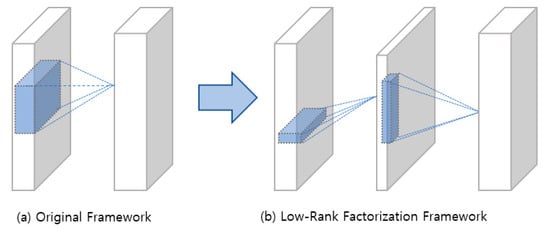
Figure 1.
Overall framework of original and the low-rank constraint convolutional layers.
2.1.2. Parameter Sharing and Pruning
The parameter sharing and pruning-based methods focus on removing noncritical and redundant parameters from deep neural networks without any significant effect on the performance using (1) quantization/binarization, (2) parameter pruning/sharing, and (3) designing structural matrix.
The original network can be compressed by network quantization, in which the number of bits required to represent each weight is reduced. Gupta et al. [8] proposed 16-bit fixed-point representation for training CNNs with a stochastic rounding scheme. It was shown in [9] that linear eight-bit quantization of the parameters can significantly accelerate training with minimal loss in terms of accuracy. Han et al. [10] proposed the method which prunes the small-weight connections first and retrains the sparsely connected networks. After that, the weights of links are quantized by weight sharing. After that, Huffman coding is applied to both the quantized weights and the codebook for further reducing the rate. First, connectivity is learned through training a normal network. After that, pruning the connections which have a small weight is done as illustrated in Figure 2. Lastly, the remaining sparse connections are fine-tuned by retraining the network. There are also many works that train CNNs with binary weights directly (e.g., BinaryNet [11], Connect [12], and XNORNetworks [13]). However, when dealing with very large CNNs (e.g., GoogLeNet [32]), the accuracy of these binarized neural networks is significantly reduced.
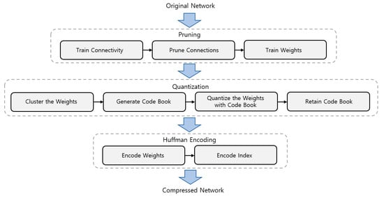
Figure 2.
A summary of the three stages in the compression pipeline proposed in [10]: pruning, quantization, and Huffman encoding. The input is the original network and the output is the compressed network.
On the other hand, several methods proposed network sharing and pruning to reduce network complexity. The work in [14] proposed a HashedNets which utilizes a lightweight hash function to randomly group weights into hash buckets for weight sharing. In [15], a structured sparsity regularizer is added on each layer to reduce channels, trivial filters, and layers. The work in [16] proposed a Neuron Importance Score Propagation (NISP) to propagate an importance score to each node and optimize the reconstruction error of the last response layer. However, all pruning criteria could be cumbersome for some applications since it requires the setup of sensitivity for layers manually.
The structural matrix can reduce the memory and also significantly accelerate the training and inference stage through gradient computations and fast matrix-vector multiplication. The work in [17] demonstrates the effectiveness of the new notion of parsimony according to the theory of structured matrices. Additionally, it can be further extended to other matrices such as block-Toeplitz matrices [18] which relate to multidimensional convolutions [19].
2.1.3. Transferred/Compact Convolutional Filters
Transferred/compact convolutional filters focus on designing structural and special convolutional filters for reducing the size of the parameter and saving storage. According to the equivariant group theory introduced in [20], the whole network models can be compressed by applying a transform to filters or layers. Besides, the computational cost can be reduced using a compact convolutional filter. The main idea is that replacing the overparametric and loose filters with compact blocks can improve the speed, which accelerates the training of CNN models on several benchmarks. Iandola et al. [21] proposed a compact neural network called SqueezeNet which stacks a bunch of fire modules. This fire module contains squeeze convolutional layers that have only 11 convolution filters which then feed into expanding layers that have both 11 and 33 convolution filters as shown in Figure 3. Szegedy et al. [22] proposed decomposing 33 convolutions into two 1 × 1 convolutions, resulting in state-of-the-art acceleration performance on the object recognition task. Other techniques include efficient and lightweight network architectures such as ShuffleNet [23], CondenseNet [24], and MobileNet [25]. These methods work well for flat/wide architectures (e.g., VGGNet [33]) but not special/narrow ones (e.g., ResNet [34] and GoogLeNet [32]) since the transfer assumptions are too strong, which leads unstable results on some datasets.
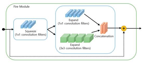
Figure 3.
Structure of the fire module in SqueezeNet [21].
2.2. Knowledge Distillation
Knowledge distillation trains a smaller compact network (student network) using the supervision signals from both ground-truth labels and a larger pretrained network (teacher network). Many methods have been proposed to minimize the performance gap between a student and a teacher. We discuss different forms of knowledge in the following categories: response-based knowledge [26,27,35], feature-based knowledge [28,29,36,37,38,39,40,41,42,43,44,45], and relation-based knowledge [30,31,46,47,48,49].
2.2.1. Response-Based Knowledge
The neural response of the final output layer in the teacher network is used in the response-based model. The basic concept is to mimic the final output of the teacher network directly. The distillation methods using response-based knowledge have been widely used in different applications and tasks due to its simplicity and effectiveness for model compression. The work in [26] shows that the student network is able to learn the complex functions of the teacher network by training the student network on the logits (the output of the last layer). Hinton et al. [27] propose to match the outputs of classifiers of student and teacher networks by minimizing the KL-divergence of the category distribution (soft target). Recently, Meng et al. [35] proposed conditional teacher-student learning, in which a student network selectively learns from either conditioned ground-truth labels or the soft target of a teacher network.
2.2.2. Feature-Based Knowledge
In feature-based knowledge distillation, the output of the intermediate (i.e., feature maps) and last layers are all utilized as knowledge for supervising the training of the student model. Romero et al. proposed FitNet [28] to mimic the intermediate feature maps of a teacher network to improve performance. However, FitNet may adversely affect the convergence and performance due to the capacity gap between student and teacher networks. The work in [29] proposed AT to transfer the attention maps which represent the relative importance of layer activations. Huang and Wang proposed Neural Selective Transfer (NST) [36] to imitate the distribution of the neuron activations from intermediate layers of the teacher network. Kim et al. proposed Factor Transfer (FT) [37] to compress features into “factors” as a more understandable form of intermediate representation using autoencoder in the teacher network, and then use a translator to extract “factors” in the student network. Heo et al. proposed Activation Boundaries (AB) [38] of the hidden neurons to force the student to learn the binarized values of the preactivation map in the teacher network. Instead of transferring knowledge by feedforward information, Czarnecki et al. [39] use gradient transfer with Sobolev training. Heo et al. proposed Boundary Supporting Sample (BSS) [40] to match the decision boundary more explicitly using an adversarial attack for discovering samples that support a decision boundary. Additionally, they use an additional boundary supporting loss which encourages the student network to match the output of the teacher network on samples close to the decision boundary. Ahn et al. proposed Variational Information Distillation (VID) [41] that maximizes a lower boundary for the mutual information between the student network and the teacher network. Heo et al. proposed Overhaul of Feature Distillation (OFD) [42] to transfer the magnitude of feature response which contains both the activation status of each neuron and feature information. Wang et al. proposed Attentive Feature Distillation (AFD) [43] which dynamically learns not only the features to transfer, but also the unimportant neurons to skip. Tian et al. proposed Contrastive Representation Distillation (CRD) [44] that maximizes a tighter lower boundary for the mutual information via a contrastive loss between the teacher network and the student network. The work in [45] proposed Deep Mutual Learning (DML) which learns in a collaborative way and teaches each other between the teacher and student networks to boost performance for both open-set and close-set problems. Any network can be either the student model or the teacher model during the training process.
2.2.3. Relation-Based Knowledge
While the output of specific layers in the teacher model is used in both response-based and feature-based knowledge, the relationships between data samples and different layers are further utilized in relation-based knowledge. To explore the relationships between different feature maps, Yim et al. proposed the Flow of Solution Procedure (FSP) [46] which is defined by the Gramian matrix (second-order statistics) across layers for transfer learning and fast optimization. They demonstrate that the FSP matrix can reflect the data flow of how to solve a problem. Passalis and Tefas proposed Probabilistic Knowledge Transfer [47] to transfer knowledge by matching the probability distribution in feature space. Park et al. proposed RKD [30] to transfer relations of data examples based on angle-wise and distance-wise distillation losses which measure structural differences in relations. The work in [48] proposed a Similarity Preserving (SP) distillation method to transfer pairwise activation similarities of input samples. Peng et al. proposed a method based on CC [31], in which the distilled knowledge contains information of instances and the correlations between two instances. Liu et al. proposed Instance Relationship Graph (IRG) [49] which contains instance features and relationships, and the feature space transformation cross layers as the knowledge to transfer.
In this paper, we take advantage of three different types of knowledge distillation to build our ensemble model as shown in Figure 4. Our proposed ensemble model consists of AT [29] as a feature-based knowledge (Figure 4A) where attention maps of intermediate layers are transferred into the student network, Logit [26] as a response-based knowledge (Figure 4B) where logits (output of the last layer) is transferred into a student network and RKD [30] as a relation-based knowledge (Figure 4C), in which relational information between the outputs of the intermediate layers is transferred into a student network.
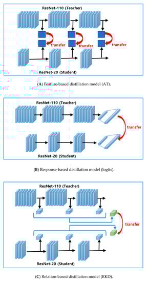
Figure 4.
Three types of knowledge distillation models used in our ensemble model.
3. Proposed Methods
In this section, the architecture of our proposed ensemble method is first presented. After that, we present the details of three key components in the following subsections.
The overall architecture of our proposed framework is illustrated in Figure 5. First, input images are augmented by the image augmentation module (Section 3.1). Second, augmented images are used as the input of three knowledge distillation models (Section 3.2). Third, the outputs of each distillation model are combined by our ensemble module to predict the category of input images (Section 3.3).
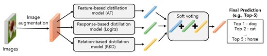
Figure 5.
Overall architecture of our proposed ensemble model.
3.1. Image Augmentation
Image augmentation as a preprocessing step of input data can improve performance and prevent overfitting. In the image augmentation step, input images are mapped into an extended space, in which all their variances are covered. Recent work has shown the effectiveness of the image augmentation method in increasing the amount of training data by augmenting our original training dataset. Additionally, the overfitting problem on training models can be reduced by augmenting training data. Our image augmentation module consists of (1) normalizing each image by mean and standard deviation, (2) randomly cropping the image to 3232 pixels size with a padding of 4, and (3) applying a random horizontal flip.
3.2. Knowledge Distillation
In our ensemble model, we use three types of individual distillation models: (1) the response-based distillation model, (2) feature-based distillation model, and (3) relation-based distillation model. Each individual distillation model is trained by minimizing its loss function. The loss function consists of the student loss between the output of the student model and ground-truth label and the distilled loss between student and teacher models for each distillation method.
3.2.1. Student Loss
First, the student loss can be calculated as the cross-entropy between the soft target of the student model estimated by softmax function and the ground-truth label as follows:
where is a ground-truth one-hot vector which represents the ground-truth label of the training dataset as 1 and all other elements are 0, and is the logit (the output of the last layer) for the i-th class of the student model.
3.2.2. Distilled Loss of the Response-Based Model
The distilled loss of response-based model using logits [26] can be calculated using the mean square error between the logits of the student model and the logits of the teacher model as follows:
The total loss of response-based model using logits is then calculated as the joint of the distilled and student losses as follows:
where is a training input, are the parameters of the student model, and α and β are the weights of the student loss and the distilled loss, respectively.
3.2.3. Distilled Loss of the Feature-Based Model
The distilled loss of feature-based model using AT [29] can be calculated as follows:
where and are the j-th pair of teacher and student attention maps in vectorized form respectively, is the indices of all student-teacher activation layer pairs for which we want to transfer attention maps, and is the l2 norm of a vector which is the square root of the sum of the absolute values squared. The total loss of the feature-based model using AT is then calculated as the joint of the distilled and student losses as follows:
3.2.4. Distilled Loss of the Relation-Based Model
The distilled loss of relation-based model using RKD [30] can be calculated as follows:
where is a set of N-tuples of distinct data examples (e.g., and ), is an n-tuple extracted from , , and are the outputs of any layer of the teacher and student network examples, respectively, is a relational potential function that measures relational properties (the angle and Euclidean distance) of the given n-tuple, and is the Huber loss that penalizes the difference between the student model and teacher model, which can be defined as follows:
In RKD, the student model is trained to mimic the relational structure of the teacher model using the relational potential function. The total loss of relation-based model using RKD is then calculated as the joint of the distilled and student losses as follows:
3.3. Ensemble of KD Models
The aim of ensemble models is to combine the prediction of several individual models in order to improve robustness and generalizability over a single individual model, thus increasing the accuracy of the model. When we try to predict the target variable using any algorithm, the main causes of the difference in predicted and actual values are variance, noise, and bias. The ensemble model helps to reduce these factors. The popular methods for ensemble learning are voting, bagging, and boosting. We adopt voting as our ensemble learning techniques since it is simple yet effective and usually recommended to complement the weakness of each individual model that generally performs well. On the other hand, other ensemble learning techniques such as bagging and boosting create very complex classifiers. Additionally, time and computation can be a bit expensive, hence unsuitable for our knowledge distillation framework in which the goal is to build a lightweight model with high performance.
The voting methods can be classified into: (1) soft voting and (2) hard voting. Soft voting is often used when an individual model can measure probabilities for the outcomes. In soft voting, the best result is obtained by averaging out the probabilities measured by individual models. On the other hand, in hard voting, the final prediction is measured by a simple majority vote. We use soft voting as our voting scheme since the output of our individual model is the probability of class membership. The final prediction of our model is then calculated using soft voting as follows:
where is the predicted category, m is the number of individual distillation models, i is the index value of the category list, and is the output of the last layer for the i-th class of the j-th distillation model.
4. Experiments and Results
To verify the suitability of our proposed method, we evaluate our method on image classification datasets. In our experiments, we adopt a ResNet-20 and ResNet-110 as student model and teacher model, respectively.
4.1. Dataset
We perform a set of experiments on two datasets, CIFAR-10 and CIFAR-100 which are widely used as the benchmarks for image classification tasks and are often used to evaluate model architectures and novel methods in the field of deep learning. CIFAR-10 consists of both 50,000 training images and 10,000 test images, from 10 classes. Each image is of size 3232 pixels. On the other hand, CIFAR-100 is a more complex dataset since it has 100 classes with 500 training images and 100 test images per class. The task for all of them is to classify images into image categories.
4.2. Experimental Settings
For a fair comparison and controlling other factors, the algorithms of other distillation methods are reproduced based on their papers and codes in Github [50] under the same conditions. In our experiment, we use Stochastic Gradient Descent (SGD) as our optimizer for all methods with Nesterov acceleration, a momentum of 0.9. The learning rate starts from 0.1 and is divided by 10 at 50% and 75% of the total epochs. Weight decay is set to 0.0005. In the training step, we augment data using our image augmentation module described in Section 3.1. The validation set is only normalized. We use the efficient ResNet-20 and ResNet-110 which has been fine-tuned to achieve high accuracy on CIFAR-10 and CIFAR-100 for all of our knowledge distillation experiments. We run each of the distillation methods for 200 epochs. We collect the highest top-k accuracy (the accuracy of the true class being equal to any of the k predicted classes) for our validation dataset for each run.
4.3. Results
The empirical results were obtained for two different datasets (CIFAR-10 and CIFAR-100) for baseline (teacher and student networks), other knowledge distillation methods discussed earlier in Section 2.2, and our proposed ensemble models with different combinations of two knowledge distillation models and three knowledge distillation models. Top-k accuracy (%) of various knowledge distillation models on CIFAR-10 and CIFAR-100 datasets is shown in Table 1 (k = 1,2 on CIFAR-10 and k = 1,5 on CIFAR-100) and Table A1 (k = 1~5 on both CIFAR-10 and CIFAR-100). In Table 1, Top-1 and Top-2 were selected on the CIFAR-10 dataset, and Top-1 and Top-5 were selected on the CIFAR-100 dataset, since Top-1 and Top-2 are commonly used metrics for the dataset with few classes (e.g., 10 classes on CIFAR-10) while Top-1 and Top-5 are commonly used metrics for the dataset with many classes (e.g., 100 classes on CIFAR-100). Additionally, the computational time for inference of the test set and the size of parameters are shown in Table 2. From Table 1 and Table 2, we found the following observations.

Table 1.
Top-k accuracy (%) of knowledge distillation models and our proposed models on the CIFAR-10 and CIFAR-100 datasets. (k = 1,2 on CIFAR-10 and k = 1,5 on CIFAR-100 where k is the number of top elements to look at for computing accuracy).
Table 2.
Computational time for inference of test set and the size of parameters.
Observation 1: Some knowledge distillation models have lower accuracy than baseline.
Analysis: From Table 1, it can be seen that some knowledge distillation methods (e.g., FSP, VID) perform worse than baseline (student network) on the CIFAR-10 dataset. These results indicate that some distillation methods based on feature-based knowledge may not generalize well and achieve unsatisfactory results in a slightly different context. This is because each distillation method is only optimized for a particular training scheme and model architecture.
Observation 2: Some relation-based knowledge distillation models have less effect on the CIFAR-100 dataset.
Analysis: From Table 1, it can be seen that some relation-based knowledge distillation methods (e.g., RKD, CC, and PKT) have less effect on the CIFAR-100 dataset. This is because there are more interclasses but fewer intra-classes in one batch. It could be alleviated by increasing the batch size or designing advanced batch sampling methods.
Observation 3: The ensemble of three models (AT, logits, and RKD) has the highest top-k accuracy among other methods in both the CIFAR-10 and CIFAR-100 datasets.
Analysis: From Table 1, it can be seen that our proposed ensemble models have the highest top-k accuracy among other models including a large teacher network on both datasets. Besides, the ensemble of only two models outperforms the teacher network in most cases. This is because our proposed ensemble methods take advantage of three types of knowledge distillation schemes which are response-based (logits), feature-based (AT), and relation-based methods (RKD).
Observation 4: Our ensemble models have less computational time for inference and less parameter size than the teacher network.
Analysis: From Table 2, it can be seen that our proposed ensemble models have less computational power than the teacher network in terms of the size of parameters and inference time. The results from Table 1 and Table 2 suggest that our ensemble model is suitable for the lightweight model with high performance for classification tasks.
5. Discussion
In this section, we discuss the comparison between our experimental results and others, the computational advantage and disadvantage of our method, and the size of training data.
5.1. Comparison between our Experimental Results and Others
Our experiment shows that several knowledge distillation models underperform one of the simple distillation methods (e.g., logits). In addition, some knowledge distillation models fail to outperform the baseline (student). The authors in [44], which implemented 10 different knowledge distillation methods, also found that all of them fail to outperform the simple knowledge distillation method (e.g., soft target). This is because most of the knowledge distillation methods are sensitive to the changes of the teacher-student pairs, and optimized for a particular training scheme, model architecture, and size. These results indicate that many knowledge distillation methods proposed by others may not generalize well and achieve poor results under different student-teacher architectures. Another potential reason is that each knowledge distillation model implemented by ours differs slightly in the design and selection of hyper-parameters from the models in the original papers. In our ensemble model, we used AT for feature-based distillation model, logits for response-based distillation model, and RKD for relation-based distillation model among other distillation models since these distillation models perform well under our student-teacher architectures as shown in Table 1, and complement each other with different types of knowledge.
5.2. Computational Advantage/Disadvantage of our Method
The computational advantage of our method is that the computational time of our proposed method is lower than the large teacher model (e.g., ResNet-110). For instance, as shown in Table 2, it took about 3.09 s for inference of the test set (10,000 images) using a large teacher model while it took about 2.53 s (ensemble of three) or 1.78 s (ensemble of two) for inference of the test set using our proposed methods. Hence, our proposed method can be used for real-time applications since it takes approximately 0.00025 s to classify each image. Besides, our proposed method still outperforms the large teacher model in terms of accuracy as shown in Table 1. In contrast, other knowledge distillation methods proposed by other authors perform worse than the large teacher model in terms of accuracy. However, our proposed method takes more computational time than other knowledge distillation methods since our method is the ensemble method which combines three lightweight models trained by three distillation methods. For training (200 epochs), it took 4600 s on CIFAR-10 and 4800 s on CIFAR-100 for each distillation method of our ensemble method with an NVIDIA GeForce GTX 1070 Ti GPU.
5.3. The Size of Training Data
The size of the training data is one of the important factors which affects the learning process. When the size of the training data is too small, it is hard to achieve good generalization performance. As a result, the accuracy of the deep learning model (e.g., ResNet-20 or 110) will be poor. In case the size of training data is not enough, the pretrained model which was previously trained on a large dataset (e.g., ImageNet [51]), can be used as a transfer learning process. In our experiment, we do not use the pretrained model since the size of the training data (CIFAR-10 and CIFAR-100) is enough.
6. Conclusions
In summary, we have presented an ensemble that combines three lightweight models learned by three different knowledge distillation strategies (feature-based, response-based, and relation-based). We evaluate our ensemble model on CIFAR-10 and CIFAR-100 which are widely used as the benchmarks for the image classification task. In our experiment, we provided an extensive evaluation of 20 different knowledge distillation and our proposed ensemble methods. Our experiment results demonstrate that our proposed ensemble model outperforms the other knowledge distillation models as well as large teacher networks. In addition, our ensemble model has less parameter size and less computational time for inference than the teacher network. These results indicate that the proposed ensemble model is suitable for the lightweight model with high performance for classification tasks. Additionally, our proposed method which is based on knowledge distillation can be applied to various tasks such as medical image segmentation [52], character animation [53,54,55], computational design [56], and object recognition [1], since knowledge distillation is not task-specific, rather a very general approach and any deep neural network architectures can be used to define both teacher (usually large network) and student (small network). For instance, CNNs [57,58,59], Long Short-Term Memory (LSTM) [60], Hidden Markov Models (HMM) [61], Dilated CNNs [62], GAN [63], and graphical model [64] can be also used to design the student and teacher networks for a specific task. Although our main focus is a model compression method using knowledge distillation which seeks to decrease the size of a particular network to run on resource-limited devices without a significant drop in accuracy, dimensionality reduction techniques [65,66,67,68] which focus on feature-level compression of input data can be also applied as the preprocessing step when handling the input data with high dimensional space or other deep learning architectures. Additionally, Restricted Boltzmann Machines (RBMs) [69,70,71] can be used to preprocess the input data in other deep learning architectures (e.g., deep autoencoder) to help the learning process become more efficient. Therefore, our proposed ensemble method can be very useful since it can be applied to other tasks and other deep neural network architectures easily, and our ensemble method can reduce the model size and at the same time enhance the performance, unlike other knowledge distillation models.
Most knowledge distillation methods focus on new distillation loss functions or new knowledge. However, the design of the student-teacher architectures is poorly investigated. In fact, apart from the distillation loss functions and knowledge, the network architectures of the student and the teacher and the relationship between them significantly influences the performance of knowledge distillation. Our experiment shows that several knowledge distillation models underperform a very simple distillation method (e.g., logits). In addition, some knowledge distillation models fail to outperform the baseline (student). These results indicate that many knowledge distillation methods may not generalize well and achieve poor results under different student-teacher architectures. As a result, the design of an effective teacher and student network architecture is still a challenging problem in knowledge distillation.
In the future, we plan to explore our proposed ensemble model with other teacher-student network architectures (e.g., AlexNet, VGG-16, ResNet-32, ResNet-50, and ResNet-110), and combine both knowledge distillation and other model compression techniques to learn effective and efficient lightweight deep learning models. Additionally, we plan to apply our ensemble model to other domains such as medical image classification and segmentation to gain more insights into the benefits of the ensemble model.
Author Contributions
Conceptualization, J.G.; methodology, J.K. and J.G.; software, J.K. and J.G.; validation, J.K. and J.G.; formal analysis, J.K. and J.G.; investigation, J.G.; resources, J.K. and J.G.; data curation, J.K.; writing—original draft preparation, J.K. and J.G.; writing—review and editing, J.K. and J.G.; visualization, J.K.; supervision, J.G.; project administration, J.G.; funding acquisition, J.G. All authors have read and agreed to the published version of the manuscript.
Funding
This research was supported by the Basic Science Research Program through the National Research Foundation of Korea (NRF) funded by the Ministry of Education (Grant No. NRF-2020R1I1A3074141) and the Brain Research Program through the NRF funded by the Ministry of Science, ICT and Future Planning (Grant No. NRF-2019M3C7A1020406).
Conflicts of Interest
The authors declare no conflict of interest.
Appendix A
Table A1.
CIFAR-10 and CIFAR-100 datasets. (k = 1~5 on both CIFAR-10 and CIFAR-100 where k is the number of top elements to look at for computing accuracy).
Table A1.
CIFAR-10 and CIFAR-100 datasets. (k = 1~5 on both CIFAR-10 and CIFAR-100 where k is the number of top elements to look at for computing accuracy).
| Method | CIFAR-10 | CIFAR-100 | ||||||||
|---|---|---|---|---|---|---|---|---|---|---|
| Top-1 | Top-2 | Top-3 | Top-4 | Top-5 | Top-1 | Top-2 | Top-3 | Top-4 | Top-5 | |
| Teacher | 94.1 | 98.06 | 99.28 | 99.67 | 99.79 | 72.69 | 83.13 | 87.95 | 90.51 | 92.25 |
| Student | 92.46 | 97.67 | 98.96 | 99.55 | 99.8 | 69.05 | 80.47 | 86.32 | 89.07 | 91.13 |
| Logits [26] | 93.14 | 97.91 | 99.15 | 99.63 | 99.82 | 70.19 | 81.96 | 87.34 | 90.23 | 92.26 |
| Soft target [27] | 92.89 | 97.68 | 99.03 | 99.61 | 99.81 | 70.42 | 81.71 | 86.93 | 90.01 | 91.81 |
| AT [29] | 93.44 | 97.86 | 99.19 | 99.69 | 99.85 | 69.69 | 81.22 | 86.46 | 89.61 | 91.41 |
| Fitnet [28] | 92.59 | 97.58 | 99.05 | 99.62 | 99.8 | 69.1 | 81.42 | 86.65 | 89.79 | 91.87 |
| NST [36] | 92.93 | 97.61 | 99.1 | 99.62 | 99.82 | 69.09 | 81.19 | 86.53 | 89.53 | 91.51 |
| PKT [47] | 93.11 | 97.89 | 99.15 | 99.48 | 99.73 | 68.96 | 80.62 | 86.06 | 89.05 | 91.03 |
| FSP [46] | 92.43 | 97.58 | 99.07 | 99.64 | 99.79 | 69.63 | 81.5 | 86.92 | 89.74 | 91.91 |
| FT [37] | 93.32 | 97.92 | 99.12 | 99.58 | 99.74 | 70.11 | 81.62 | 87.09 | 90.16 | 91.83 |
| RKD [30] | 93.21 | 97.91 | 99.14 | 99.5 | 99.76 | 69.32 | 81.19 | 86.35 | 89.35 | 91.33 |
| AB [38] | 93.04 | 97.56 | 99.08 | 99.62 | 99.78 | 69.66 | 81.37 | 86.64 | 89.72 | 91.51 |
| SP [48] | 92.97 | 97.71 | 99.13 | 99.65 | 99.85 | 70.09 | 81.61 | 86.74 | 89.92 | 91.79 |
| Sobolev [39] | 92.62 | 97.63 | 98.96 | 99.57 | 99.81 | 68.53 | 80.96 | 86.61 | 89.81 | 91.78 |
| BSS [40] | 92.56 | 97.67 | 99.01 | 99.53 | 99.79 | 69.57 | 81.59 | 87.13 | 90.17 | 92.01 |
| CC [31] | 92.74 | 97.62 | 99.16 | 99.6 | 99.8 | 69.06 | 80.87 | 86.12 | 89.48 | 91.4 |
| IRG [49] | 93.05 | 97.99 | 99.14 | 99.62 | 99.81 | 69.88 | 81.63 | 86.87 | 89.92 | 91.64 |
| VID [41] | 92.37 | 97.6 | 99.04 | 99.59 | 99.84 | 68.84 | 80.83 | 86.3 | 89.47 | 91.38 |
| OFD [42] | 92.86 | 97.52 | 98.92 | 99.54 | 99.82 | 69.77 | 81.4 | 86.86 | 89.98 | 91.85 |
| AFD [43] | 92.96 | 97.75 | 99.03 | 99.51 | 99.78 | 68.86 | 80.77 | 86.29 | 89.54 | 91.6 |
| CRD [44] | 92.67 | 97.76 | 99.03 | 99.61 | 99.81 | 71.01 | 81.99 | 87.53 | 90.19 | 92.17 |
| DML [45] | 92.87 | 97.88 | 99.21 | 99.71 | 99.87 | 70.53 | 82.43 | 87.44 | 90.05 | 92.02 |
| Ens-AT-Logits | 93.97 | 98.14 | 99.36 | 99.73 | 99.91 | 73.61 | 84.7 | 89.29 | 91.87 | 93.49 |
| Ens-RKD-Logits | 93.82 | 98.26 | 99.32 | 99.67 | 99.8 | 73.32 | 84.39 | 89.08 | 91.64 | 93.41 |
| Ens-AT-RKD | 94.16 | 98.18 | 99.37 | 99.69 | 99.84 | 73.75 | 84.27 | 89.04 | 91.73 | 93.39 |
| Ens-all | 94.41 | 98.32 | 99.42 | 99.74 | 99.92 | 74.55 | 85.53 | 89.88 | 92.34 | 94.07 |
References
- Krizhevsky, A.; Sutskever, I.; Hinton, G.E. Imagenet classification with deep convolutional neural networks. In Advances in Neural Information Processing Systems; MIT Press: Cambrige, UK, 2012; pp. 1097–1105. [Google Scholar]
- Voulodimos, A.; Doulamis, N.; Doulamis, A.; Protopapadakis, E. Deep learning for computer vision: A brief review. Comput. Intell. Neurosci. 2018, 2018, 1–13. [Google Scholar] [CrossRef]
- Silver, D.; Huang, A.; Maddison, C.J.; Guez, A.; Sifre, L.; Van Den Driessche, G.; Schrittwieser, J.; Antonoglou, I.; Panneershelvam, V.; Lanctot, M.; et al. Mastering the game of Go with deep neural networks and tree search. Nature 2016, 529, 484–489. [Google Scholar] [CrossRef]
- Devlin, J.; Chang, M.W.; Lee, K.; Toutanova, K. Bert: Pre-training of deep bidirectional transformers for language understanding. arXiv 2018, arXiv:1810.04805. [Google Scholar]
- Lebedev, V.; Ganin, Y.; Rakhuba, M.; Oseledets, I.; Lempitsky, V. Speeding-up convolutional neural networks using fine-tuned cp-decomposition. arXiv 2014, arXiv:1412.6553. [Google Scholar]
- Tai, C.; Xiao, T.; Zhang, Y.; Wang, X. Convolutional neural networks with low-rank regularization. arXiv 2015, arXiv:1511.06067. [Google Scholar]
- Ioffe, S.; Szegedy, C. Batch normalization: Accelerating deep network training by reducing internal covariate shift. arXiv 2015, arXiv:1502.03167. [Google Scholar]
- Gupta, S.; Agrawal, A.; Gopalakrishnan, K.; Narayanan, P. Deep learning with limited numerical precision. In Proceedings of the 32nd International Conference on Machine Learning, Lille, France, 6–11 July 2015; Volume 37, pp. 1737–1746. [Google Scholar]
- Vanhoucke, V.; Senior, A.; Mao, M.Z. Improving the speed of neural networks on CPUs. In Proceedings of the NIPS Workshop on Deep Learning and Unsupervised Feature Learning, Granada, Spain, 12–17 December 2011. [Google Scholar]
- Han, S.; Mao, H.; Dally, W.J. Deep compression: Compressing deep neural networks with pruning, trained quantization and Huffman coding. arXiv 2015, arXiv:1510.00149. [Google Scholar]
- Courbariaux, M.; Bengio, Y. Binarynet: Training deep neural networks with weights and activations constrained to +1 or −1. arXiv 2016, arXiv:1602.02830. [Google Scholar]
- Courbariaux, M.; Bengio, Y.; David, J.P. Binaryconnect: Training deep neural networks with binary weights during propagations. In Advances in Neural Information Processing Systems; MIT Press: Cambrige, UK, 2015; pp. 3123–3131. [Google Scholar]
- Rastegari, M.; Ordonez, V.; Redmon, J.; Farhadi, A. Xnor-net: Imagenet classification using binary convolutional neural networks. In Proceedings of the European Conference on Computer Vision, Amsterdam, The Netherlands, 8–16 October 2016; Springer: Cham, Switzerland; pp. 525–542. [Google Scholar]
- Chen, W.; Wilson, J.; Tyree, S.; Weinberger, K.; Chen, Y. Compressing neural networks with the hashing trick. In Proceedings of the 32nd International Conference on International Conference on Machine Learning, Lille, France, 6–11 July 2015; pp. 2285–2294. [Google Scholar]
- Wen, W.; Wu, C.; Wang, Y.; Chen, Y.; Li, H. Learning structured sparsity in deep neural networks. In Advances in Neural Information Processing Systems; NIPS Proceedings: Red Hook, NY, USA, 2016; pp. 2074–2082. [Google Scholar]
- Yu, R.; Li, A.; Chen, C.F.; Lai, J.H.; Morariu, V.I.; Han, X.; Gao, M.; Lin, C.Y.; Davis, L.S. Nisp: Pruning networks using neuron importance score propagation. In Proceedings of the IEEE Conference on Computer Vision and Pattern Recognition, Salt Lake City, UT, USA, 18–23 June 2018; pp. 9194–9203. [Google Scholar]
- Sindhwani, V.; Sainath, T.; Kumar, S. Structured transforms for small-footprint deep learning. In Advances in Neural Information Processing Systems; NIPS Proceedings: Red Hook, NY, USA, 2015; pp. 3088–3096. [Google Scholar]
- Kailath, T.; Chun, J. Generalized displacement structure for block-Toeplitz, Toeplitz-block, and Toeplitz-derived matrices. SIAM J. Matrix Anal. Appl. 1994, 15, 114–128. [Google Scholar] [CrossRef]
- Rakhuba, M.V.; Oseledets, I.V. Fast multidimensional convolution in low-rank tensor formats via cross approximation. SIAM J. Sci. Comput. 2015, 37, A565–A582. [Google Scholar] [CrossRef][Green Version]
- Cohen, T.; Welling, M. Group equivariant convolutional networks. In Proceedings of the 33rd International Conference on Machine Learning, New York, NY, USA, 19–24 June 2016; pp. 2990–2999. [Google Scholar]
- Iandola, F.N.; Han, S.; Moskewicz, M.W.; Ashraf, K.; Dally, W.J.; Keutzer, K. SqueezeNet: AlexNet-level accuracy with 50x fewer parameters and <0.5 MB model size. arXiv 2016, arXiv:1602.07360. [Google Scholar]
- Szegedy, C.; Ioffe, S.; Vanhoucke, V.; Alemi, A. Inception-v4, Inception-ResNet and the impact of residual connections on learning. arXiv 2016, arXiv:1602.07261. [Google Scholar]
- Zhang, X.; Zhou, X.; Lin, M.; Sun, J. Shufflenet: An extremely efficient convolutional neural network for mobile devices. In Proceedings of the IEEE Conference on Computer Vision and Pattern Recognition, Salt Lake City, UT, USA, 18–22 June 2018; pp. 6848–6856. [Google Scholar]
- Huang, G.; Liu, S.; Van der Maaten, L.; Weinberger, K.Q. Condensenet: An efficient DenseNet using learned group convolutions. In Proceedings of the IEEE Conference on Computer Vision and Pattern Recognition, Salt Lake City, UT, USA, 18–22 June 2018; pp. 2752–2761. [Google Scholar]
- Howard, A.G.; Zhu, M.; Chen, B.; Kalenichenko, D.; Wang, W.; Weyand, T.; Andreetto, M.; Adam, H. Mobilenets: Efficient convolutional neural networks for mobile vision applications. arXiv 2017, arXiv:1704.04861. [Google Scholar]
- Ba, L.J.; Caruana, R. Do deep nets really need to be deep? In Advances in Neural Information Processing Systems; NIPS Proceedings: Red Hook, NY, USA, 2014; pp. 2654–2662. [Google Scholar]
- Hinton, G.; Vinyals, O.; Dean, J. Distilling the knowledge in a neural network. arXiv 2015, arXiv:1503.02531. [Google Scholar]
- Romero, A.; Ballas, N.; Kahou, S.E.; Chassang, A.; Gatta, C.; Bengio, Y. FitNets: Hints for thin deep nets. arXiv 2015, arXiv:1412.6550. [Google Scholar]
- Zagoruyko, S.; Komodakis, N. Paying more attention to attention: Improving the performance of convolutional neural networks via attention transfer. arXiv 2017, arXiv:1612.03928. [Google Scholar]
- Park, W.; Kim, D.; Lu, Y.; Cho, M. Relational knowledge distillation. In Proceedings of the IEEE Conference on Computer Vision and Pattern Recognition, Long Beach, CA, USA, 16–20 June 2019; pp. 3967–3976. [Google Scholar]
- Peng, B.; Jin, X.; Liu, J.; Li, D.; Wu, Y.; Liu, Y.; Zhou, S.; Zhang, Z. Correlation congruence for knowledge distillation. In Proceedings of the IEEE International Conference on Computer Vision, Seoul, Korea, 27 October–2 November 2019; pp. 5007–5016. [Google Scholar]
- Szegedy, C.; Liu, W.; Jia, Y.; Sermanet, P.; Reed, S.; Anguelov, D.; Erhan, D.; Vanhoucke, V.; Rabinovich, A. Going deeper with convolutions. In Proceedings of the IEEE Conference On Computer Vision and Pattern Recognition, Boston, MA, USA, 7–12 June 2015; pp. 1–9. [Google Scholar]
- Simonyan, K.; Zisserman, A. Very deep convolutional networks for large-scale image recognition. arXiv 2014, arXiv:1409.1556. [Google Scholar]
- He, K.; Zhang, X.; Ren, S.; Sun, J. Deep residual learning for image recognition. In Proceedings of the IEEE Conference on Computer Vision and Pattern Recognition, Las Vegas, NV, USA, 27–30 June 2016; pp. 770–778. [Google Scholar]
- Meng, Z.; Li, J.; Zhao, Y.; Gong, Y. Conditional teacher-student learning. In Proceedings of the 44th International Conference on Acoustics, Speech and Signal Processing, Brighton, UK, 12–17 May 2019; pp. 6445–6449. [Google Scholar]
- Huang, Z.; Wang, N. Like what you like: Knowledge distill via neuron selectivity transfer. arXiv 2017, arXiv:1707.01219. [Google Scholar]
- Kim, J.; Park, S.; Kwak, N. Paraphrasing complex network: Network compression via factor transfer. In Advances in Neural Information Processing Systems; NIPS Proceedings: Red Hook, NY, USA, 2018; pp. 2760–2769. [Google Scholar]
- Heo, B.; Lee, M.; Yun, S.; Choi, J.Y. Knowledge transfer via distillation of activation boundaries formed by hidden neurons. In Proceedings of the AAAI Conference on Artificial Intelligence, New Orleans, LA, USA, 2–7 February 2018; Volume 33, pp. 3779–3787. [Google Scholar]
- Czarnecki, W.M.; Osindero, S.; Jaderberg, M.; Swirszcz, G.; Pascanu, R. Sobolev training for neural networks. In Advances in Neural Information Processing Systems; NIPS Proceedings: Red Hook, NY, USA, 2017; pp. 4278–4287. [Google Scholar]
- Heo, B.; Lee, M.; Yuno, S.; Choi, J.Y. Knowledge distillation with adversarial samples supporting decision boundary. In Proceedings of the AAAI Conference on Artificial Intelligence, New Orleans, LA, USA, 2–7 February 2018; Volume 33, pp. 3771–3778. [Google Scholar]
- Ahn, S.; Hu, S.X.; Damianou, A.; Lawrence, N.D.; Dai, Z. Variational information distillation for knowledge transfer. In Proceedings of the IEEE Conference on Computer Vision and Pattern Recognition, Long Beach, CA, USA, 16–20 June 2019; pp. 9163–9171. [Google Scholar]
- Heo, B.; Kim, J.; Yun, S.; Park, H.; Kwak, N.; Choi, J.Y. A comprehensive overhaul of feature distillation. In Proceedings of the IEEE International Conference on Computer Vision, Seoul, Korea, 27 October–2 November 2019; pp. 1921–1930. [Google Scholar]
- Wang, K.; Gao, X.; Zhao, Y.; Li, X.; Dou, D.; Xu, C. Pay attention to features, transfer learn faster CNNs. In Proceedings of the International Conference on Learning Representations, Addis Ababa, Ethiopia, 26–30 April 2020; Available online: https://openreview.net/forum?id=ryxyCeHtPB (accessed on 4 July 2020).
- Tian, Y.; Krishnan, D.; Isola, P. Contrastive representation distillation. arXiv 2019, arXiv:1910.10699. [Google Scholar]
- Zhang, Y.; Xiang, T.; Hospedales, T.M.; Lu, H. Deep mutual learning. In Proceedings of the IEEE Conference on Computer Vision and Pattern Recognition, Salt Lake City, UT, USA, 18–23 June 2018; pp. 4320–4328. [Google Scholar]
- Yim, J.; Joo, D.; Bae, J.; Kim, J. A gift from knowledge distillation: Fast optimization, network minimization and transfer learning. In Proceedings of the IEEE Conference on Computer Vision and Pattern Recognition, Honolulu, HI, USA, 21–26 July 2017; pp. 4133–4141. [Google Scholar]
- Passalis, N.; Tefas, A. Learning deep representations with probabilistic knowledge transfer. In Proceedings of the European Conference on Computer Vision (ECCV), Munich, Germany, 8–14 September 2018; pp. 268–284. [Google Scholar]
- Tung, F.; Mori, G. Similarity-preserving knowledge distillation. In Proceedings of the IEEE International Conference on Computer Vision, Seoul, Korea, 27 October–2 November 2019; pp. 1365–1374. [Google Scholar]
- Liu, Y.; Cao, J.; Li, B.; Yuan, C.; Hu, W.; Li, Y.; Duan, Y. Knowledge distillation via instance relationship graph. In Proceedings of the IEEE Conference on Computer Vision and Pattern Recognition, Long Beach, CA, USA, 16–20 June 2019; pp. 7096–7104. [Google Scholar]
- Github. Available online: https://github.com/AberHu/Knowledge-Distillation-Zoo (accessed on 2 July 2020).
- Russakovsky, O.; Deng, J.; Su, H.; Krause, J.; Satheesh, S.; Ma, S.; Huang, Z.; Karpathy, A.; Khosla, A.; Bernstein, M.; et al. Imagenet large scale visual recognition challenge. Int. J. Comput. Vis. 2015, 115, 211–252. [Google Scholar] [CrossRef]
- Rachmadi, M.F.; Valdés-Hernández, M.D.C.; Agan, M.L.F.; Di Perri, C.; Komura, T. Segmentation of white matter hyperintensities using convolutional neural networks with global spatial information in routine clinical brain MRI with none or mild vascular pathology. Comput. Med. Imaging Graph. 2018, 66, 28–43. [Google Scholar] [CrossRef]
- Holden, D.; Komura, T.; Saito, J. Phase-functioned neural networks for character control. ACM Trans. Graph. (TOG) 2017, 36, 1–13. [Google Scholar] [CrossRef]
- Mousas, C.; Newbury, P.; Anagnostopoulos, C.N. Evaluating the covariance matrix constraints for data-driven statistical human motion reconstruction. In Proceedings of the 30th Spring Conference on Computer Graphics, Smolenice, Slovakia, 28–30 May 2014; pp. 99–106. [Google Scholar]
- Mousas, C.; Newbury, P.; Anagnostopoulos, C.N. Data-driven motion reconstruction using local regression models. In Proceedings of the 10th International Conference Artificial Intelligence Applications and Innovations, Rhodes, Greece, 19–21 September 2014; pp. 364–374. [Google Scholar]
- Suk, H.I.; Wee, C.Y.; Lee, S.W.; Shen, D. State-space model with deep learning for functional dynamics estimation in resting-state fMRI. NeuroImage 2016, 129, 292–307. [Google Scholar] [CrossRef] [PubMed]
- Chéron, G.; Laptev, I.; Schmid, C. P-cnn: Pose-based cnn features for action recognition. In Proceedings of the IEEE international conference on computer vision, Santiago, Chile, 7–13 December 2015; pp. 3218–3226. [Google Scholar]
- Saito, S.; Wei, L.; Hu, L.; Nagano, K.; Li, H. Photorealistic facial texture inference using deep neural networks. In Proceedings of the IEEE Conference on Computer Vision and Pattern Recognition, Honolulu, HI, USA, 21–26 July 2017; pp. 5144–5153. [Google Scholar]
- Li, R.; Si, D.; Zeng, T.; Ji, S.; He, J. Deep convolutional neural networks for detecting secondary structures in protein density maps from cryo-electron microscopy. In Proceedings of the IEEE International Conference on Bioinformatics and Biomedicine (BIBM), Shenzhen, China, 15–18 December 2016; pp. 41–46. [Google Scholar]
- Li, Z.; Zhou, Y.; Xiao, S.; He, C.; Huang, Z.; Li, H. Auto-conditioned recurrent networks for extended complex human motion synthesis. arXiv 2017, arXiv:1707.05363. [Google Scholar]
- Abdel-Hamid, O.; Mohamed, A.R.; Jiang, H.; Penn, G. Applying Convolutional Neural Networks Concepts to Hybrid NN-HMM Model For Speech Recognition. In Proceedings of the IEEE International Conference on Acoustics, speech and signal processing (ICASSP), Kyoto, Japan, 25–30 March 2012; pp. 4277–4280. [Google Scholar]
- Rekabdar, B.; Mousas, C. Dilated Convolutional Neural Network for Predicting Driver’s Activity. In Proceedings of the 21st International Conference on Intelligent Transportation Systems (ITSC), Maui, HI, USA, 4–7 November 2018; pp. 3245–3250. [Google Scholar]
- Rekabdar, B.; Mousas, C.; Gupta, B. Generative adversarial network with policy gradient for text summarization. In Proceedings of the IEEE 13th International Conference on Semantic Computing (ICSC), Newport Beach, CA, USA, 30 January–1 February 2019; pp. 204–207. [Google Scholar]
- Bilmes, J.A.; Bartels, C. Graphical model architectures for speech recognition. IEEE Signal Process. Mag. 2005, 22, 89–100. [Google Scholar] [CrossRef]
- Tenenbaum, J.B.; De Silva, V.; Langford, J.C. A global geometric framework for nonlinear dimensionality reduction. Science 2000, 290, 2319–2323. [Google Scholar] [CrossRef]
- Cao, L.J.; Chua, K.S.; Chong, W.K.; Lee, H.P.; Gu, Q.M. A comparison of PCA, KPCA and ICA for dimensionality reduction in support vector machine. Neurocomputing 2003, 55, 321–336. [Google Scholar] [CrossRef]
- Roweis, S.T.; Saul, L.K. Nonlinear dimensionality reduction by locally linear embedding. Science 2000, 290, 2323–2326. [Google Scholar] [CrossRef]
- Belkin, M.; Niyogi, P. Laplacian eigenmaps for dimensionality reduction and data representation. Neural Comput. 2003, 15, 1373–1396. [Google Scholar] [CrossRef]
- Ngiam, J.; Khosla, A.; Kim, M.; Nam, J.; Lee, H.; Ng, A.Y. Multimodal deep learning. In Proceedings of the 28th International Conference on Machine Learning, Bellevue, WA, USA, 28 June–2 July 2011. [Google Scholar]
- Nam, J.; Herrera, J.; Slaney, M.; Smith, J.O., III. Learning Sparse Feature Representations for Music Annotation and Retrieval. In Proceedings of the 13th International Society for Music Information Retrieval Conference, Porto, Portugal, 8–12 October 2012; pp. 565–570. [Google Scholar]
- Mousas, C.; Anagnostopoulos, C.N. Learning motion features for example-based finger motion estimation for virtual characters. 3D Res. 2017, 8, 25. [Google Scholar] [CrossRef]


© 2020 by the authors. Licensee MDPI, Basel, Switzerland. This article is an open access article distributed under the terms and conditions of the Creative Commons Attribution (CC BY) license (http://creativecommons.org/licenses/by/4.0/).