Abstract
Anti-aliasing plays a decisive role in enhancing immersion experience in games and 3D visualization fields. In general, hardware anti-aliasing is not directly compatible with deferred shading. It is challenging to detect geometry edges accurately from sub-pixel to alleviate artifacts. In this paper, we propose an anti-aliasing algorithm of the #-filter anti-aliasing based on sub-pixel continuous edges. It can solve the geometry edges aliasing and the flicker problem in deferred shading. First, the geometry scene with multi-sampling anti-aliasing (MSAA) is rendered to a G-Buffer designed elaborately. Second, the geometry edges are detected on the sub-pixel-level. We mainly take advantage of the Chebyshev inequality to adaptively determine the edges from the probability statistic and the view frustum location. Third, the continuous geometry edges are reconstructed by a #-filter method. Finally, the edge pixels are shaded adaptively. The implementation demonstrates that our algorithm is efficient and scalable for generating high-quality anti-aliasing geometry and reducing shading calculation overhead.
1. Introduction
Anti-aliasing techniques play an essential role in games and 3D simulation applications to enhance immersion and reduce visual discomfort. They can solve the inharmonious factors: jaggies or scintillation. Furthermore, the main reason is that the screen image shows the discrete pixels after the rasterization. It is difficult to reconstruct the continuous edges because continuous information is lost in deferred shading. Still, the current common computer hardware cannot achieve high-precision rendering power.
In the early forward rendering, super-sampling anti-aliasing (SSAA), multi-sampling anti-aliasing (MSAA), and coverage-sampling anti-aliasing (CSAA) can be built-in hardware to improve the performance and effect of the image. Subsequently, the post-processing anti-aliasing [1] gradually becomes popular. Still, the forward rendering anti-aliasing is not compatible with deferred shading technology [2] because the geometry information lost after rasterization. For example, in such a context, MSAA will be degenerated to SSAA and decrease its performance advantages.
However, the geometry edges’ reconstruction is difficult to be obtained accurately in deferred shading. The challenge is significant for our anti-aliasing method, demonstrating how to render the anti-aliasing geometry in deferred shading. According to the critical steps of our algorithm, the main contributions of our algorithm are as follows:
- A novel method of edges detection is proposed. Edge pixels are determined by probability statistics and the object’s location in the view frustum. It can fill in the stencil buffer to identify whether it is an edge pixel. Normal pixels can be shaded quickly to improve the whole rendering performance.
- The continuous sub-pixel edges are reconstructed by the #-filter method according to the whole geometry edges. Only one sub-pixel covered by fragment is processed to reconstruct the continuous edges and minimize the calculation overhead.
- The hardware anti-aliasing with deferred shading works with our algorithm to increase the flexibility and extensibility. Moreover, the normal and edge pixels are independently and adaptively shaded to solve shading thread consistency.
2. Related Work
In general, the aliasing problem is processed by the two anti-aliasing methods. One is to improve the rendering resolution, increasing the scene sampling; the other is to sample the image area and make the edge smooth. The ultimate purpose of anti-aliasing methods is to balance effectiveness and efficiency. To achieve the best trade-off, the academia and the industry have made many efforts in the field [3,4].
Forward rendering is a standard graphics rendering technique. Each light source is calculated for each vertex and fragment. The forward rendering anti-aliasing typically includes SSAA [5], MSAA [6], CSAA [7], and so on. Meanwhile, these anti-aliasing techniques have been embedded in the hardware to accelerate graphic rendering. Although the classical approach MSAA can be very costly depending on the complexity of the shading and the overall quality is not as good as SSAA, it is much faster. MSAA only handles the edge polygons of the model, so the overhead is greatly reduced. CSAA is an optimization algorithm based on MSAA. The memory capacity and bandwidth requirements in the anti-aliasing process are reduced. Decoupled coverage anti-aliasing (DCAA) [8] improves upon MSAA by further decoupling coverage from visibility for high-quality geometry anti-aliasing.
The deferred shading postpones the geometry object’s shading to the final level of the pipeline, adds the hidden surface before shading, saves the rendering of the geometry color, normal, and coordinates through the G-Buffer, and completes the illumination calculation once. The basic idea of the post-processing anti-aliasing is to detect discontinuities on the image and blur the jagged edges. While the approach is not entirely new [9,10,11], some advanced algorithms have only been applied recently in games [12,13,14]. More refined solutions like directionally blur localized anti-aliasing (DLAA) [15], use smarter blurs that produce very natural results and functional temporal coherence. Nevertheless, these approaches still yield blurrier results than MSAA. A filter-based method called morphological anti-aliasing (MLAA) [16,17] does not need multiple samples and can efficiently be implemented on the CPU. Deverly et al. [18] introduce an efficient MLAA algorithm running on medium-range GPUs. A lot of anti-aliasing methods of MLAA are based on image morphology detection of post-processing techniques, including fast approximate anti-aliasing (FXAA) [19], distance to edge anti-aliasing (DEAA) [20], DLAA, sub-pixel reconstruction anti-aliasing (SRAA) [2], sub-pixel morphological anti-aliasing (SMAA) [21], and so on.
If there is a way to detect geometry edges, it can also enable MSAA in deferred shading. Geometry post-process anti-aliasing (GPAA) [22] algorithms compute feature pixels. However, the algorithms above cannot handle sub-pixel-level aliasing artifacts correctly. Only screen resolution geometry information is adopted. Sub-pixel reconstruction anti-aliasing (SRAA) combines a screen-resolution shading image with the additional super-sampling position, depth, or normal G-Buffers. It is capable of reconstructing sub-pixel-level geometry details. Furthermore, Jorge et al. [21] show how to combine MLAA with MSAA or SSAA for accurate sub-pixel features, and how to couple it with temporal re-projection, and always preserving the sharpness of the image.
Deferred shading hands large numbers of lights and post-process. Deferred Shading with MSAA [23] (DSM for short) demonstrates how to implement MSAA on top of deferred shading. The general idea is to first render the scene geometry to a multi-sample-enabled G-Buffer. Then it determines which pixels are complex and finally performs shading adaptively. Similarly, triangle-based geometry anti-aliasing (TGAA) [24] stores the coverage information into a screen-resolution bitmask. It can address the memory problem of storage and overheads.
Meanwhile, temporal anti-aliasing (TAA) [25,26] is the primary method for game anti-aliasing today because it does handle well both geometry edges and interior shaded content. This has been state-of-the-art for about the last decade. Therefore, the challenge is significant for our anti-aliasing method to reconstruct accurate geometry edges.
3. Algorithm and Features
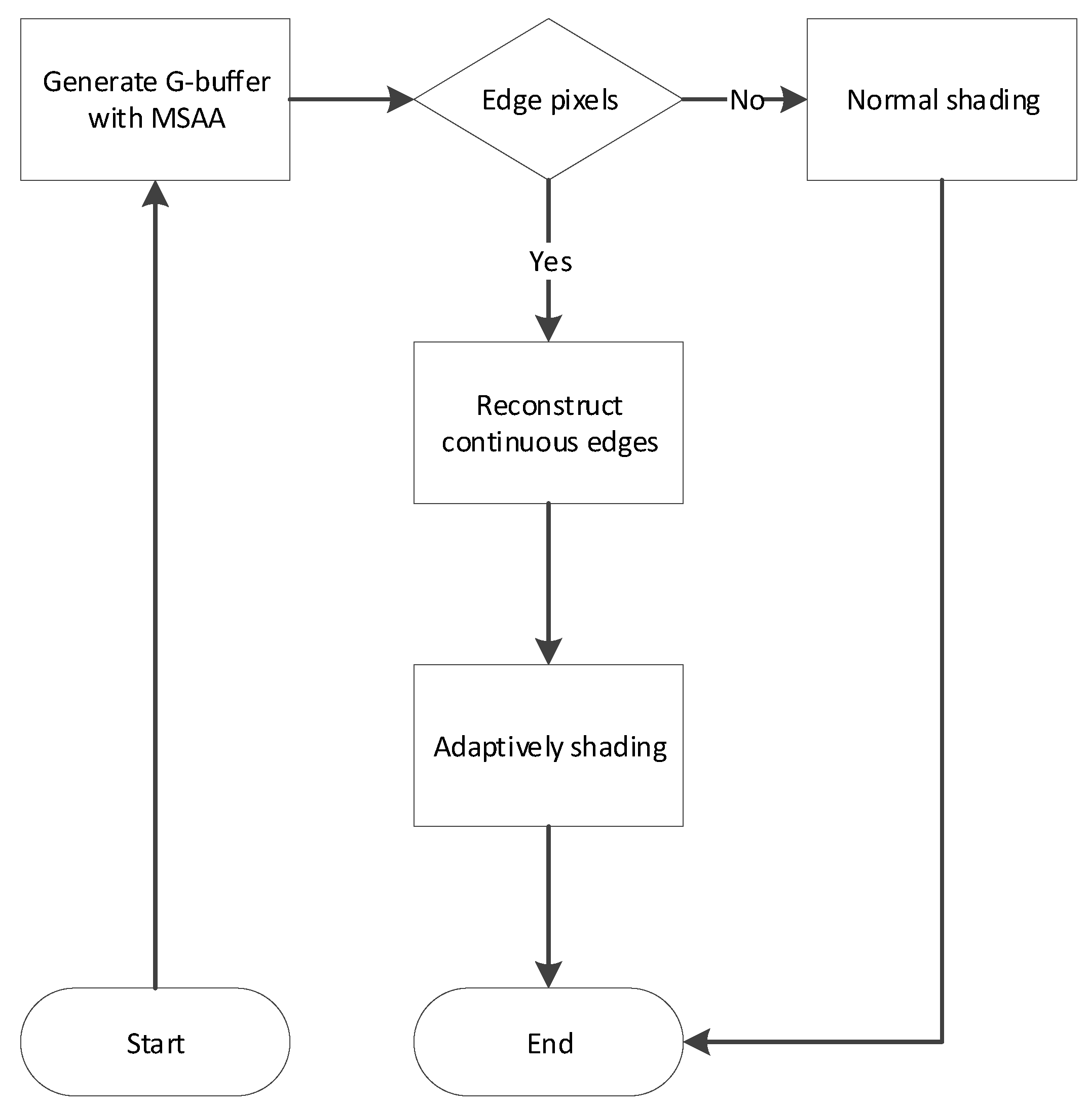
The deferred shading is currently mainstream rendering mode. However, the hardware anti-aliasing is not directly compatible with the deferred shading. In order to use MSAA to improve the rendering effect, we use these theories of the integrity of statistics and visual perception to reconstruct continuous geometry edges in deferred shading. The algorithm is shown in Figure 1. There are four critical steps in the algorithm:

Figure 1.
The process of the algorithm.
- Generate G-Buffer with MSAA: G-Buffer only stores necessary information to reduce calculation overhead, especially anti-aliasing and transparency rendering information.
- Determine edge pixels: The geometry edges are determined on the sub-pixel. Moreover, the normal pixels and edge pixels are separated. It mainly takes advantage of the Chebyshev inequality to adaptively detect the edges from the probability statistic and the position in the view frustum.
- Reconstruct continuous edges: The continuous geometry edges are reconstructed from the sub-pixel-level and a whole. Furthermore, edge pixels covered only one fragment will be restored, which will maximize the performance without reducing the rendering effect.
- Adaptively shading: The edge pixels of adaptive can effectively reduce calculation overhead and improve anti-aliasing quality. Meanwhile, the normal pixels are quickly shaded.
The algorithm mainly improves the GPU rendering capability to reduce the thread coherency. Normal pixels perform shading once but would have to wait for edges pixels to complete. Meanwhile, the algorithm reconstructs more reliable continuous geometry edges for sub-pixel anti-aliasing. The algorithm key features are as follows.
3.1. Render Scene Geometry to G-Buffer
G-Buffer generally includes the necessary information that will be taken part in illumination calculation in deferred shading, such as depth, normal, diffuse, and specular attributes. We have designed five render targets (see Table 1) to fill in G-Buffer. The different geometry information is respectively stored in four channels under each render target. Several important G-Buffer information are described as follows.

Table 1.
G-Buffer information. Five render targets are used and four channels under each render target respectively store different geometry information.
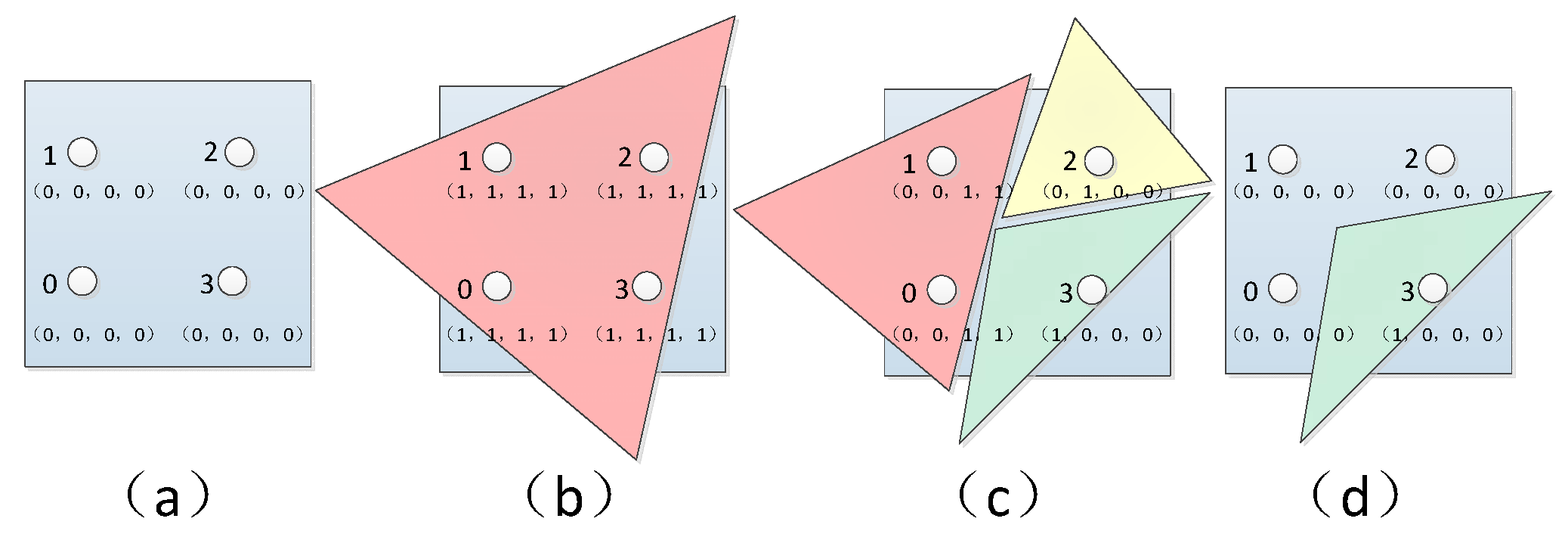
- Coverage information: The G channel of the RT2 stores coverage, which is the sample mask of each sub-pixel with MSAA, as shown in Figure 2. The geometry edges usually happen in more than one unique fragment (see Figure 2c), and one sub-pixel covered by one fragment (see Figure 2d), rather than no fragment pixel (See Figure 2a) or all covered by one fragment (see Figure 2b).
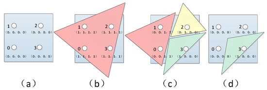 Figure 2. The sample mask of the current fragment.
 - Depth information: The non-linear depth will result in higher accuracy near the camera but lower accuracy far away from the camera. We make a linear transform for the non-linear depth () under the perspective projection, as in (1). Meanwhile, linear depth helps to eliminate the z-fighting (depth struggle over the same depth) caused by far away from the camera. Moreover, the actual 3D pixel position can be calculated through the depth and the parameters of the viewport projection matrix (2).where f and n respectively are the far clip plane and the near clip plane; and are the position of fragment; and are the width and height of window; is the inverse of projection matrix.The B channel of the RT1 stores the transparent mask. It can effectively handle the geometry aliasing. The alpha value processes the rendering of the transparent object. Meanwhile, R and G channels only store X and Y components of the normal, so the Z component can be restored through Equation (3), where x and y are normalized values of normal X and Y components. Some of the other channels for rendering targets store scene color information such as colors, lighting, and shadows.
3.2. Separate Normal and Edge Pixels
DSM shows two approaches to determine edge pixels. The can very efficiently detect complex pixels. Still, it does have a drawback of marking some non-edge pixels as complex since it relies on underlying geometry rather than screen space discontinuities. Therefore, we mainly adopt the screen space discontinuities to separate normal and edges pixels, similar to extracting more geometry features [27].
Due to the thread shading coherency, the edge pixels will be separated from the normal pixels. Though the discontinuities can be checked by normal, color, and depth between samples, it is not accurate and self-adaptive. The Chebyshev inequality is used in the variance shadow map (VSM) algorithm [28] to estimate the expectation of each pixel depth and the expectation of the square of the depth. Furthermore, suppose the depth value is smaller than expected in the shadow calculation stage. In that case, it is in light, otherwise in shadow. Although the idea is used to generate soft shadows, Chebyshev inequality’s effective edges processing method inspires us to detect edge pixels. Next, we mainly use the one-tailed version of Chebyshev inequality, namely Cantelelli’s inequality, to detect whether a sub-pixel belongs to the edge pixel.
Chebyshev inequality can be used to determine the edges and reduce edge jaggies and scintillation. The more the random variable X deviates from , the smaller its probability. Furthermore, the distribution of random variables is unknown, and only the limits of probability (4) can be estimated in the case of and . Specifically, we use the sampled pixel depth as the unknown random variable X. All sub-pixel depths are used to calculate the expectation and variance . Therefore, any X exceeding every untreated depth t is no more than value t to calculate each pixel’s probability (5). The formula is proved in VSM.
where t is the current pixel depth, is the expectation of sub-pixel depths, and is the variance of sub-pixel depths.
The scene objects are large in the near distance under the perspective projection, but small in the far distance. A more explicit edge requires more pixels to represent it, whether in the near or the far. Therefore, judging the edges of the scene geometry, the similar LOD is used to determine the edge pixels adaptively. It provides a crucial step in dealing with edge anti-aliasing and flickering in the distance. Therefore, the threshold is expressed, as in (6). As the sample number of MSAA increases, the smaller the threshold, the more edges are detected; as the pixel depth increases, the larger the threshold, reducing unnecessary scintillation.
where P is the probability value by the Chebyshev inequality, N is the sample number of MSAA; z is the depth of the current fragment, f and n respectively are the far clip plane and the near clip plane.
3.3. Reconstruct Continuous Edge and Adaptively Shade
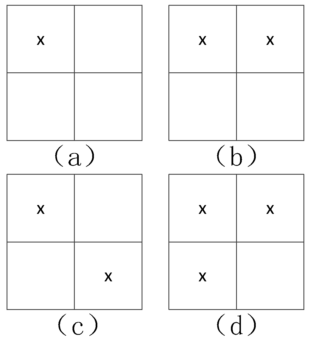
The geometry edges are the places where anti-aliasing should be most often done. Therefore, it is vital to search for the continuous edge for shading adaptively in deferred shading. The four conditions of edge pixels are determined from the sub-pixel (see Figure 3). Only the sub-pixel covered by a fragment is processed to reconstruct the continuous edge as a whole and other conditions. It will maximize performance without reducing the effect. The number of unique coverage masks per pixel is counted. Each unique fragment in pixels using the number of samples is weighted. For example, there are three unique fragments (see Figure 2c). The red fragment is weighted 2/4, while the yellow and green fragments are each weighted 1/4.

Figure 3.
The four modes of edge pixels based on sub-pixel.
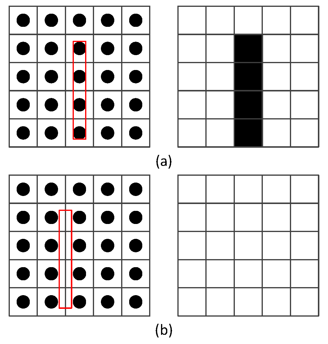
When a display object is relatively smaller, it is prone to distortion. The rectangle at the center of the pixel can be sampled to be widened display (see Figure 4a), and the rectangle cannot be sampled to disappear (see Figure 4b). This loss of detail in the time-varying scene is prone to flicker artifacts. Meanwhile, the frame discontinuity can suffer from flickering, primarily due to a failure to balance history rejection and ghosting [26,29].
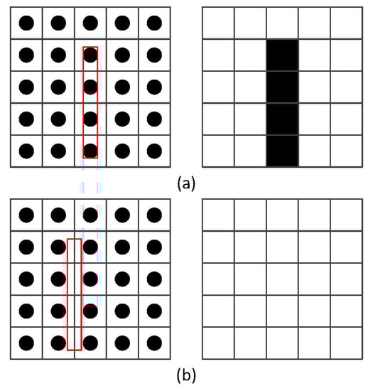
Figure 4.
The flickering phenomenon.
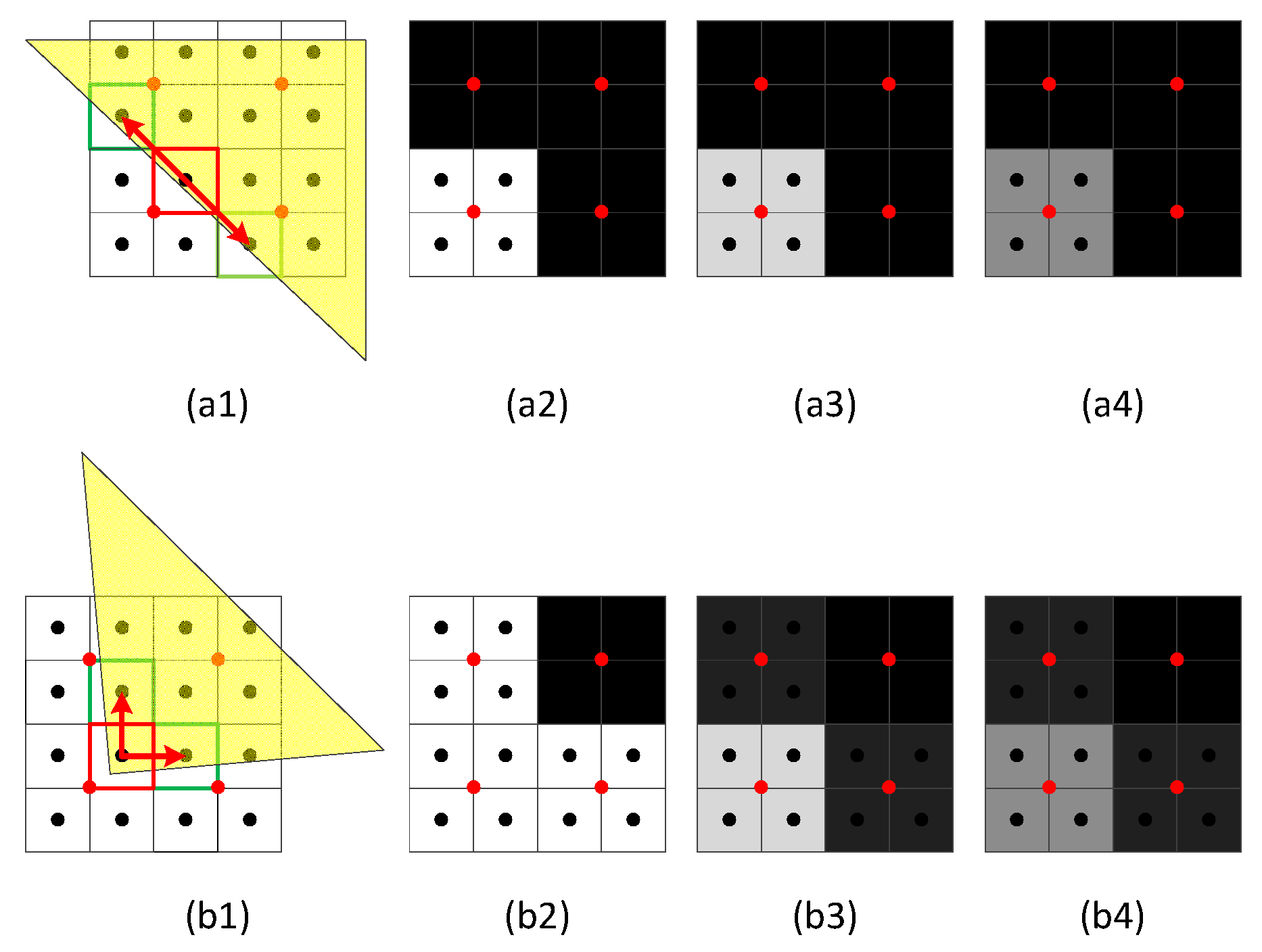
Anti-aliasing aims to smooth the edges of the geometry scene and to reduce flicker when moving. A pixel only has a limited message, despite multi-sampling focuses on sub-pixel. The sample is considered on the whole continuous edge. The two shading conditions of one sub-pixel covered by the fragment in different sample ways are shown in Figure 5. Compared with the anti-aliasing shading of the single pixel, the shading result is closer to the practical geometry condition from the neighboring sub-pixel (see Figure 5(a4,b4)). For example, the common sub-pixel anti-aliasing only focuses on the local pixels rather than the whole edge pixels. It will lose the detail of the edges. Meanwhile, more pixels can build more accurate sub-pixel edges, but it will increase performance. Usually, four neighborhood samples are enough to balance performance and effect.

Figure 5.
The continuous edges. The red point is the pixel center, and the black is the sub-pixel center. (a1) and (b1) are the different cases of the four pixels and sixteen sub-pixels covered by a yellow fragment. (a2) and (b2) are no anti-aliasing. (a3) and (b3) are the common sub-pixel anti-aliasing. (a4) and (b4) are our method to deal with the sub-pixel anti-aliasing.
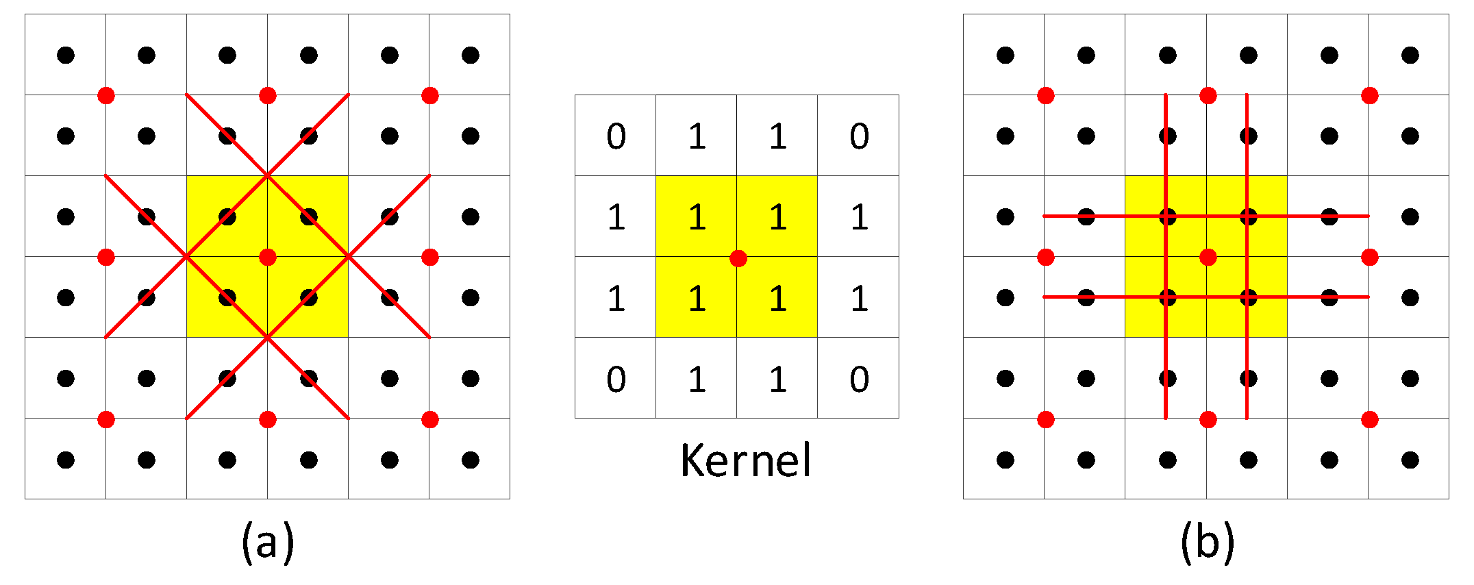
Therefore, the #-filter method (see Figure 6) is to complete the above results. There are two modes to determine the single sub-pixel and to shade adaptively. Figure 6a aims at Figure 5(b1) and Figure 6b aims at Figure 5(a1). One sub-pixel shading only happens in one line of the #-filter. Meanwhile, the #-filter is represented by an array with the weights, and the color c of each pixel is calculated by adjacent sub-pixels , as in (7). The weight of #-filter is an array of size n, and only 12 sub-pixels are used in the four samples. In order to improve the calculation performance, we currently use the kernel, as shown in Figure 5(middle), but the kernel can be expanded according to rendering requirements. Each sub-pixel point with 1 in the #-filter kernel is multiplied by edge value (6) to determine whether it is a geometry edge as a whole. Moreover, the common filtering methods can be used as weights, such as low pass filtering, high pass filtering, directional filtering, Laplacian filtering, and Gaussian filtering.
where the e is the edge value, 0 is not an edge and 1 is an edge; are the weights of #-filter array of size n; is the color of adjacent sub-pixels.
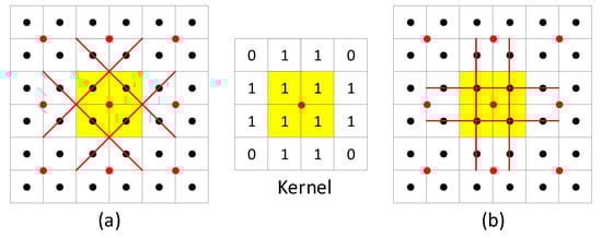
Figure 6.
The #-filter method. (a) corresponds to Figure 5(a1), and (b) to (b1).
4. Results
The proposed anti-aliasing algorithm has been implemented on a PC with Intel(R) Core(TM) i7-4790@3.6GHz, 16 GB of physical memory, and NVIDIA GeForce GTX970 GPU, 4 GB memory. The Windows 10 operating system is used, and the OpenGL library with GLSL language is used as a 3D rendering interface. All the following tests employ the resolution 1080 × 720 to render the scenes with geometry models. Some experimental data are from public datasets [30].
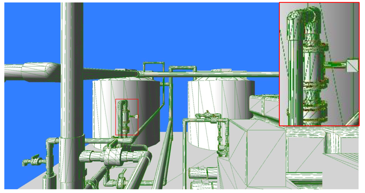
In the step of determining edge pixels, our method can obtain more edges than the depth discontinuity method in Figure 7. It is attributed to the idea of probability and statistics to determine the maximum extent of the edge pixels. Compared with DSM, which can efficiently detect complicated pixels, it does have a drawback of marking some non-edge pixels as complex. Another approach is to search for discontinuities, but some geometry edges are not determined conclusively in Figure 7b.
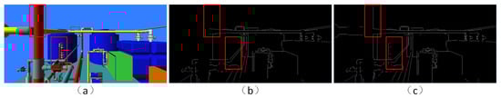
Figure 7.
Depth edges. The red box marks the difference in the actual image (a). (b) is the depth discontinuity method. (c) is our method.
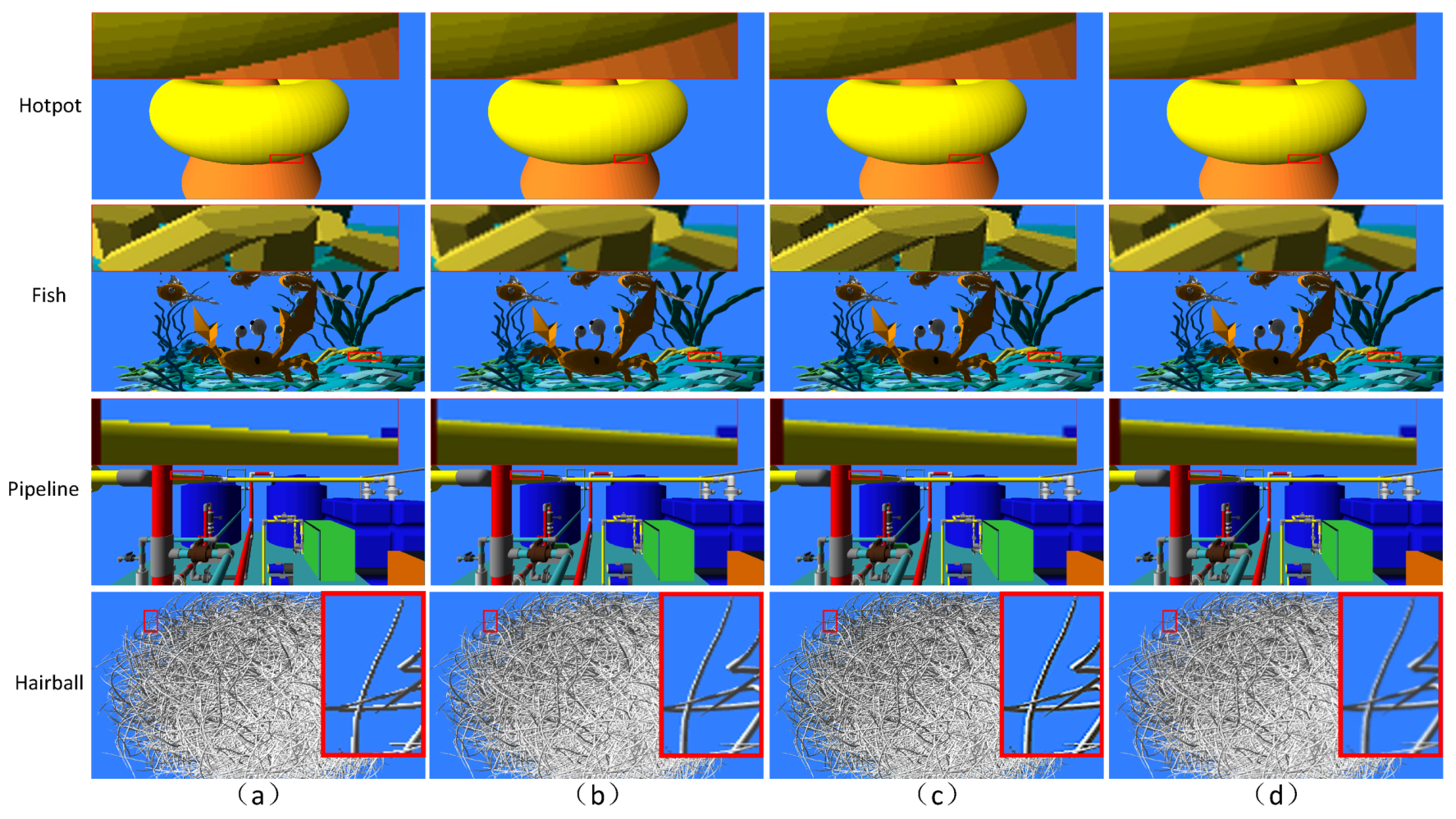
On the one hand, the adaptive shading of the complex pixels is adopted in Figure 8. On the other hand, the #-filter method is used to shade to reach the anti-aliasing effects adaptively. The Figure 9 presents comparisons among the no AA (a), deferred shading with MSAA (DSM for short) (b), simple discontinuity (c), and ours (d) in four scenes of different triangle numbers. Our algorithm has obvious improvement in the aliasing and achieves a better effect as with other algorithms.
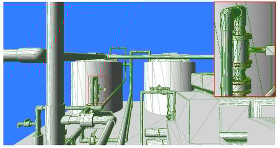
Figure 8.
Color-coded edge complex pixels based on unique fragment counts. Green means two fragments, blue means three, and red means four.
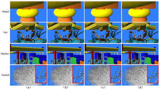
Figure 9.
The different anti-aliasing algorithms. The complexity of the scene is sorted from low to high, ranking Hotpot (Tri:20,190), Fish (Tri:66,694), Pipeline (Tri:83,746), and Hairball (Tri:2,880,000). (a) is no anti-aliasing (AA), (b) is DSM, (c) is the simple discontinuity method, and (d) is our algorithm.
The algorithm implements 4x MSAA, but the idea can be easily extended to support more sample counts. However, the sample count relies on the practical application to decide. Meanwhile, we verify the performance in Figure 10, while the video card closes the vertical synchronization. Although our algorithm has a lower rate of 20%–30% in the whole rendering pipeline, it has to do with the edge determine and the adaptive shading. Some performance can be sacrificed in exchange for better results. This algorithm can also achieve the purpose of the real-time application. The higher the hardware configuration, the more reliable the rendering performance.
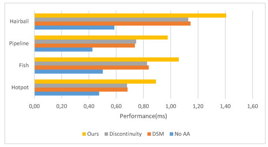
Figure 10.
The performance (ms) of several anti-aliasing methods at different scenes.
Meanwhile, no AA, FXAA, temporal AA, and our methods with 4x MSAA are compared in the scene Sponza (Tri:262,267), as shown in Figure 11. The anti-aliasing effect of various methods has been greatly improved, but the improvement effect is different. FXAA is a fast shader-based post-processing technique applied to any program, including those that do not support other hardware-based anti-aliasing forms. FXAA can be used in conjunction with other anti-aliasing methods to improve overall image quality. Temporal AA works by reprogramming coverage sample locations across pixels within the same frame and across frames. This has the effect of making the overall sample pattern irregular, which eliminates aliasing artifacts. Our method is used to minimize the “stair-step” effect sometimes seen along 3D objects’ edges. Though our method cannot process non-edges, it can combine the post-processing or TAA to enhance the anti-aliasing effects. In terms of performance overhead, their rendering times are (a) 0.0115 ms, (b) 0.0121 ms, (c) 0.0130 ms, and (d) 0.0137 ms, respectively. In order to accurately detect the edges from the sub-pixel, the time cost is higher than other methods.
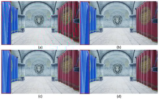
Figure 11.
The effect contrast of no AA (a), FAXX (b), temporal anti-aliasing (TAA) (c), and our method (d).
5. Conclusions and Future Work
In our method, hardware-supported multiple sampling is used to oversample geometry scenes to refine anti-aliasing in deferred shading. The following advantages or methods are used to render high-quality anti-aliasing images. First, Chebyshev inequality is utilized to detect the edges from the statistics and visual perception. Second, the normal pixels and edge pixels are separated. Third, the geometry edges are reconstructed by the #-filter method. Finally, the complicated edge pixels are shaded adaptively. Our further work will concentrate on the render of the transparency objects and other detail combined art-of-core post-posting and temporal anti-aliasing. Furthermore, more refined and more effective edges are reconstructed by a learning-based #-filter method.
Author Contributions
Methodology, D.L.; project administration, D.L.; supervision, J.Z.; validation, D.L.; writing—original draft, D.L.; writing—review and editing, J.Z. All authors have read and agreed to the published version of the manuscript.
Funding
This research received no external funding.
Conflicts of Interest
The authors declare no conflict of interest.
References
- Jimenez, J.; Gutierrez, D.; Yang, J.; Reshetov, A.; Demoreuille, P.; Berghoff, T.; Perthuis, C.; Yu, H.; McGuire, M.; Lottes, T.; et al. Filtering approaches for real-time anti-aliasing. ACM SIGGRAPH Courses 2011, 2, 4. [Google Scholar]
- Chajdas, M.G.; McGuire, M.; Luebke, D. Subpixel reconstruction antialiasing for deferred shading. In Proceedings of the Symposium on Interactive 3D Graphics and Games, San Francisco, CA, USA, 18–20 February 2011; pp. 15–22. [Google Scholar]
- Maule, M.; Comba, J.L.; Torchelsen, R.; Bastos, R. Transparency and anti-aliasing techniques for real-time rendering. In Proceedings of the 2012 25th SIBGRAPI Conference on Graphics, Patterns and Images Tutorials, Ouro Preto, Brazil, 22–25 August 2012; IEEE: Ouro Preto, Brazil, 2012; pp. 50–59. [Google Scholar]
- Clarberg, P.; Toth, R.; Munkberg, J. A sort-based deferred shading architecture for decoupled sampling. ACM Trans. Graph. (TOG) 2013, 32, 1–10. [Google Scholar] [CrossRef]
- Haeberli, P.; Akeley, K. The accumulation buffer: Hardware support for high-quality rendering. ACM SIGGRAPH Comput. Graph. 1990, 24, 309–318. [Google Scholar] [CrossRef]
- Iourcha, K.; Yang, J.C.; Pomianowski, A. A directionally adaptive edge anti-aliasing filter. In Proceedings of the Conference on High Performance Graphics 2009, New Orleans, LA, USA, 1–3 August 2009; pp. 127–133. [Google Scholar]
- Young, P. Coverage Sampled Antialiasing; NVIDIA Corporation Technical Report; NVIDIA Corporation: Santa Clara, CA, USA, 2006. [Google Scholar]
- Wang, Y.; Wyman, C.; He, Y.; Sen, P. Decoupled coverage anti-aliasing. In Proceedings of the 7th Conference on High-Performance Graphics, Los Angeles, CA, USA, 7–9 August 2015; pp. 33–42. [Google Scholar]
- Bloomenthal, J. Edge inference with applications to antialiasing. ACM SIGGRAPH Comput. Graph. 1983, 17, 157–162. [Google Scholar] [CrossRef]
- Salvi, M.; Vidimče, K. Surface based anti-aliasing. In Proceedings of the ACM SIGGRAPH Symposium on Interactive 3D Graphics and Games, Costa Mesa, CA, USA, 9–11 March 2012; pp. 159–164. [Google Scholar]
- Holländer, M.; Boubekeur, T.; Eisemann, E. Adaptive supersampling for deferred anti-aliasing. J. Comput. Graph. Tech. (JCGT) 2013, 2, 2. [Google Scholar]
- Crassin, C.; McGuire, M.; Fatahalian, K.; Lefohn, A. Aggregate G-buffer anti-aliasing. In Proceedings of the 19th Symposium on Interactive 3D Graphics and Games, San Francisco, CA, USA, 27 February–1 March 2015; pp. 109–119. [Google Scholar]
- Sung, M.; Choi, S. Selective Anti-Aliasing for Virtual Reality Based on Saliency Map. In Proceedings of the 2017 International Symposium on Ubiquitous Virtual Reality (ISUVR), Nara, Japan, 27–29 June 2017; IEEE: Nara, Japan, 2017; pp. 16–19. [Google Scholar]
- Nah, J.H.; Ki, S.; Lim, Y.; Park, J.; Shin, C. AXAA: Adaptive approximate anti-aliasing. In ACM SIGGRAPH 2016 Posters; ACM: New York, NY, USA, 2016; p. 51. [Google Scholar]
- Andreev, D. Directionally localized anti-aliasing (DLAA). In Game Developers Conference; GDC: San Francisco, CA, USA, 2011; Volume 2, p. 4. [Google Scholar]
- Reshetov, A. Morphological antialiasing. In Proceedings of the Conference on High Performance Graphics 2009, New Orleans, LA, USA, 1–3 August 2009; pp. 109–116. [Google Scholar]
- Jimenez, J.; Masia, B.; Echevarria, J.I.; Navarro, F.; Gutierrez, D. Practical Morphological Antialiasing. In GPU Pro 360 Guide to Rendering; AK Peters/CRC Press: Boca Raton, FL, USA, 2018; pp. 135–153. [Google Scholar]
- Biri, V.; Herubel, A.; Deverly, S. Practical morphological antialiasing on the GPU. In ACM SIGGRAPH 2010 Talks; ACM: New York, NY, USA, 2010; p. 1. [Google Scholar]
- Lottes, T. Fxaa. In White Paper; NVIDIA Corporation Technical Report; Nvidia: Santa Clara, CA, USA, February 2009. [Google Scholar]
- Malan, H. Distance-to-edge anti-aliasing. In ACM SIGGRAPH Courses Presentation; ACM: New York, NY, USA, 2011. [Google Scholar]
- Jimenez, J.; Echevarria, J.I.; Sousa, T.; Gutierrez, D. SMAA: Enhanced subpixel morphological antialiasing. In Computer Graphics Forum; Wiley Online Library: Hoboken, NJ, USA, 2012; Volume 31, pp. 355–364. [Google Scholar]
- Persson, E. Geometric Post-Process Anti-Aliasing. 2011. Available online: http://humus.name/index.php (accessed on 3 February 2020).
- NVIDIA. Antialiased Deferred Rendering. Available online: http://docs.nvidia.com/gameworks/content/gameworkslibrary/graphicssamples/d3d_samples/antialiaseddeferredrendering.htm (accessed on 3 February 2020).
- Du, W.; Feng, J.; Yang, B. Sub-Pixel Anti-Aliasing Via Triangle-Based Geometry Reconstruction. In Computer Graphics Forum; Wiley Online Library: Hoboken, NJ, USA, 2014; Volume 33, pp. 81–90. [Google Scholar]
- Schied, C.; Peters, C.; Dachsbacher, C. Gradient estimation for real-time adaptive temporal filtering. Proc. ACM Comput. Graph. Interact. Tech. 2018, 1, 1–16. [Google Scholar]
- Yang, L.; Liu, S.; Salvi, M. A Survey of Temporal Antialiasing Techniques. STAR 2020, 39. Available online: https://behindthepixels.io/assets/files/TemporalAA.pdf (accessed on 9 February 2020). [CrossRef]
- Bazazian, D.; Casas, J.R.; Ruiz-Hidalgo, J. Fast and robust edge extraction in unorganized point clouds. In Proceedings of the 2015 International Conference on Digital Image Computing: Techniques and Applications (DICTA), Adelaide, Australia, 23–25 November 2015; IEEE: Adelaide, Australia, 2015; pp. 1–8. [Google Scholar]
- Yang, B.; Dong, Z.; Feng, J.; Seidel, H.P.; Kautz, J. Variance soft shadow mapping. In Computer Graphics Forum; Wiley Online Library: Hoboken, NJ, USA, 2010; Volume 29, pp. 2127–2134. [Google Scholar]
- Marrs, A.; Spjut, J.; Gruen, H.; Sathe, R.; McGuire, M. Adaptive temporal antialiasing. In Proceedings of the Conference on High-Performance Graphics, Vancouver, BC, Canada, 10–12 August 2018; pp. 1–4. [Google Scholar]
- McGuire, M. Computer Graphics Archive. 2017. Available online: https://casual-effects.com/data (accessed on 12 August 2020).


© 2020 by the authors. Licensee MDPI, Basel, Switzerland. This article is an open access article distributed under the terms and conditions of the Creative Commons Attribution (CC BY) license (http://creativecommons.org/licenses/by/4.0/).