CBRR Model for Predicting the Dynamics of the COVID-19 Epidemic in Real Time

Abstract

Because of the lack of reliable information on the spread parameters of COVID-19, there is an increasing demand for new approaches to efficiently predict the dynamics of new virus spread under uncertainty. The study presented in this paper is based on the Case-Based Reasoning method used in statistical analysis, forecasting and decision making in the field of public health and epidemiology. A new mathematical Case-Based Rate Reasoning model (CBRR) has been built for the short-term forecasting of coronavirus spread dynamics under uncertainty. The model allows for predicting future values of the increase in the percentage of new cases for a period of 2–3 weeks. Information on the dynamics of the total number of infected people in previous periods in Italy, Spain, France, and the United Kingdom was used. Simulation results confirmed the possibility of using the proposed approach for constructing short-term forecasts of coronavirus spread dynamics. The main finding of this study is that using the proposed approach for Russia showed that the deviation of the predicted total number of confirmed cases from the actual one was within 0.3%. For the USA, the deviation was 0.23%.

1. Introduction

The prediction of the novel coronavirus COVID-19 dynamics is inevitably associated with the lack of statistics from previous years and the need to adequately use the currently available information on the developing epidemic parameters, for which the degree of uncertainty is extremely high. Many research groups in the USA, China, and Europe are working on the development of effective models and methods for predicting the spread of the new virus in the short term [1,2,3,4,5]. Models for predicting the peaks and duration of the COVID-19 epidemic have already been presented in leading periodical scientific journals [6,7,8,9,10].

The existing large-dimensional deterministic models of the Susceptible-Infected-Recovered (SIR) or Susceptible-Exposed-Infected-Recovered (SEIR) type [11,12,13] are built based on the mechanisms of virus spread from individual to individual. They use epidemiological parameter estimates of known viruses, which is hardly suitable for modeling a new type of viral epidemic. Apart from the epidemiological models, various time series models are proposed in order to model and predict the coronavirus dynamics [14,15]. In addition, one can see an increase in the number of models based on machine learning techniques. For example, the authors of the study [16] evaluated the performance of a dynamic Bayesian network in infectious disease surveillance. In the article [17], a dynamic neural network model for predicting the risk of Zika virus in real time is developed. The main condition for all mentioned approaches is the availability of a sufficient amount of historical data. Data from previous periods are required to build forecast models suitable for use in national systems for monitoring and controlling the epidemic dynamics. However, because of the lack of data on the development of the new coronavirus epidemic a year or more ago, only statistical data from the time intervals immediately preceding the current moment can be used. In such a situation, the Case-Based Reasoning method [18] is apparently the most acceptable, the earlier version of which is the Method of Analogues [19]. This approach has showed good performance in different areas. For example, the authors of [20] showed that case-based reasoning is a promising methodology for assisting conceptual product design and monitoring new product development (NDP) projects. They propose to apply such an approach towards using neural networks to estimate the cost of NPD. In [21], a case-based reasoning approach in combination with a Bayesian optimization algorithm is used for solving optimization problems. At the same time, until recently, this approach was not widely applied in the field of dynamic processes forecasting. Schmidt and Waligora in [18] compared the statistical approach that is often used in practice and the precedent method that they developed, using statistics from the previous time periods, as well as the current data. They convincingly demonstrated the advantage of their method in predicting the dynamics of an influenza epidemic, in which waves are characterized by irregular cycles that are hard to predict using previous epidemic statistics.

2. Materials and Methods

2.1. Related Works

Currently, in journals and on the Internet, one can find various mathematical models predicting the dynamics of new cases of COVID-19 [3,4,6,7,8,10,11,12,13,14,15,22]. In [3], the authors provided estimates of the epidemic scale in Wuhan and other cities, including outside mainland China, to which the virus could have been spread from Wuhan. The authors predicted the values of internal and global public health risks from epidemics based on the use of the SEIR model, taking into account possible scenarios of preventive interventions. In [6], the dynamics of coronavirus spread in India was studied using a system of differential equations with constant coefficients and the concept of a basic reproductive number, using Pontryagin’s maximum principle to solve the problem of optimizing preventive measures. In [10], attention was drawn to the similarity of the dynamics of the total number of infected, recovered, and dead people in China and Italy. It also analyzed the solutions to the system of differential equations adopted in the Susceptible-Infected-Recovered-Deaths (SIRD) model. It is noted by the authors that although the SIRD model is rather crude, its use gives a good chance to reflect at least the general features of the epidemic evolution. The proposed methodology is aimed at predicting the onset of the peak in the growth of new infections and the number of deaths in Italy for the entire period of the epidemic. The authors of [10] showed that the trajectories generated by the SIRD model are very sensitive to variations in its parameters, which significantly reduces the quality of forecasting, especially over a long-term time horizon. In [7], a spatio-temporal approach was considered, based on the use of Brownian motion and the SBDiEM (Stereographic Brownian Diffusion Epidemiology Model) model for predicting the dynamics of infection. It was proposed to be used for creating a system for monitoring and countering pandemics using artificial intelligence technologies. The authors of [8] used a quantitative picture of the spread of COVID-19 disease in China as a test case and infection statistics data from eight countries to assess the evolution of the epidemiological process in each of these countries. This approach is based on the Gaussian hypothesis of virus spread and the SIR basic model.

It should be noted that the SIR family models are good for simulating situations in the case of standard infectious diseases, for example, influenza. When a new infection appears, the lack of reliable information on the duration of the incubation period, the value of the reproductive number, mortality, and other parameters makes it difficult to use this type of model. In [13], the deviation of the modeling results from real data was at least 7%. According to the forecast for Italy, 238,465 cases were expected by 13 September 2020, while, on 20 August, there were already more than 256,000 cases. In [14], the development of the epidemic in 15 countries was considered. In particular, the authors presented a forecast that the number of cases in Italy by 7 July 2020, would reach 400,000 people. According to official data, as of this date, 241,956 people were observed, i.e., the deviation was 65.3%. In [22], an adapted SIR model was presented to predict the course of the epidemic in Portugal, with peak values estimated to range from 7000 to 13,000. In fact, the peak observed on 10 April 2020, was 1516 cases, which was significantly lower.

Given the difficulties in using deterministic models such as SIR, SEIR, SIRD to predict the dynamics of the spread of COVID-19, which use estimates of the parameters of the spread of known viruses, the development of alternative methods for assessing the spread of the epidemic of a new virus is an extremely topical issue.

2.2. Preliminary Insight on Recurrent Relations

The official statistics provided by the Center for Systems Science and Engineering (CSSE) at Johns Hopkins University [23] present daily data on the total number of confirmed cases of $I\left(t\right)$ (Infected) on the current day t, number of recovered individuals $R\left(t\right)$ (Recovered), number of deaths $D\left(t\right)$, and the number of currently active cases $A\left(t\right)$. Let us note that the following balanced condition $I\left(t\right)=A\left(t\right)+R\left(t\right)+D\left(t\right)$ holds for any current day. In [10], the authors showed that, in the time window 22 January–15 March 2020, the following day-by-day patterns took place for China, Italy, and France

$$P\left(t+1\right)=\alpha {\left[P\left(t\right)\right]}^{\beta }, t\in \left\{1,2,\dots ,T\right\},$$

(1)

where $P=\left(I,R,D\right)$. This observation allows for the assumption that there is some universality in epidemic spreading dynamics within each country. It leads to the idea that simple models of the mean-field type can be adopted to describe epidemic spreading in time irrespective of the specific country of interest. Authors propose to describe epidemic evolution by the following system of differential Equation (2):

$$\begin{array}{l}\frac{dS}{dt}=-\rho \cdot S\cdot I,\\ \frac{dI}{dt}=\rho \cdot S\cdot I-\left(a+d\right)\cdot I,\\ \frac{dR}{dt}=a\cdot I,\\ \frac{dD}{dt}=d\cdot I,\end{array}$$

(2)

with given initial conditions for some initial time. Parameter $\rho$ is the infection rate, while $a$ and $d$ are recovery and death rates, respectively. Average values of the best-fit parameters and associated standard deviations were obtained from 30 independent runs of the stochastic differential evolution algorithm. The analysis of SIRD model implementation revealed that the recovery rate is the same for Italy and China, while infection and death rates appear to be different. The SIRD model has placed the peak in Italy around 21 March 2020. This matches actual data. The model predicted the maximum number of active cases about 26,000 at the peak of the outbreak, with the number of deaths at the end of the epidemics about 18,000. Unfortunately, this prediction failed. The actual number of active cases in Italy on 21 March 2020, according to data from [23], was more than twice higher. The number of deaths was higher than 18,000 on 9 April 2020 and appeared to be 33,500 on 1 June 2020.

2.3. Case-Based Rate Reasoning Method

Thinking about the disadvantages of the SIRD model for forecasting COVID-19 dynamics, we considered the possibility to model future epidemic evolution based on the idea of some universality in epidemic spreading dynamics within each country expressed in Formula (1). The total number of confirmed cases $I\left(t\right)$ can be represented in the form (3):

$$I\left(t\right)=\alpha \left(t\right)\times I\left(t-1\right),$$

(3)

where $\alpha \left(t\right)\ge 0$ is a growing factor of the total number of confirmed cases on day t. For example, the total number of confirmed cases increased by 7% at day t has a growth factor of 1.07.

We represent $\alpha \left(t\right)$ in the following form: $\alpha \left(t\right)=1+\frac{r\left(t\right)}{100}.$

In our model, we consider $r\left(t\right)$ as a key parameter determining the dynamics of $I\left(t\right)$ and call it the percentage growth rate of new confirmed cases recorded on day $t\in \left\{1,2,\dots ,T\right\}$. The formula used for calculation $r\left(t\right)$ is the number new cases on day $t$ divided by the total number of cases on the previous day $t-1$ and multiplied by 100.

Let the time horizon of the development of the epidemic be divided into M intervals $\left(T_{m-1},T_m\right]$, $0\le T_{m-1}<T_m\le T$, $m=1,2,\dots ,M$. Then, for any interval $\left(T_{m-1},T_m\right]$ and any $k=1,2,\dots ,\left(T_m-T_{m-1}\right)$, the dynamics of the number of infected can be presented as follows (4):

$$I\left(T_{m-1}+k\right)=\left(1+\frac{r\left(T_{m-1}+k\right)}{100}\right)\times I\left(T_{m-1}+k-1\right), k=1,2,\dots ,\left(T_m-T_{m-1}\right).$$

(4)

Therefore, the following expression (5) is true for the total number of infected at the end of the given interval:

$$I\left(T_m\right)=\left(1+\frac{r\left(T_{m-1}+1\right)}{100}\right)\times \left(1+\frac{r\left(T_{m-1}+2\right)}{100}\right)\times \cdots \times \left(1+\frac{r\left(T_m\right)}{100}\right)\times I\left(T_{m-1}\right).$$

(5)

To build the predicted trajectory in the proposed CBRR (Case-Based Rate Reasoning) model on a given $T_{m-1}$ and interval $\left(T_{m-1},T_m\right]$, a sequence of predicted rate values $\tilde{r}\left(T_{m-1}+k\right)$ and a value of $T_m$ are generated and the predicted value of the statistic indicators in future periods is determined.

The proposed model can be considered a special case of a predictive dynamic regression model (PDRM) [24] for forecasting $\tilde{r}\left(T_{m-1}+k\right)$ on the interval $\left(T_{m-1},T_m\right]$ with a fixed level ${\tilde{r}}_m$ and random input parameter $T_m$. Probabilistic properties of the input parameter $T_m$ are characterized by the corresponding parameters of spreading processes in country-predecessors. The corresponding equation for predicted percentage growth has the following form (6):

$$\begin{array}{l}\tilde{r}\left(T_{m-1}+k\right)=\tilde{r}\left(T_{m-1}+k-1\right)-A^{\left(k\right)}\left(\tilde{r}\left(T_{m-1}\right)-{\tilde{r}}_m\right),\\ k=1,2,\dots \end{array}$$

(6)

with deterministic or random values $A^{\left(k\right)}\in \left[0,1\right]$ which satisfy balance condition (7):

$${\displaystyle {\sum }_{k=1}^{T_m-T_{m-1}}{A}^{\left(k\right)}}=1 .$$

(7)

In the present study, we use uniformly distributed values (8):

$$A^{\left(k\right)}=\frac{1}{T_m-T_{m-1}}, k=1,2,\dots ,\left(T_m-T_{m-1}\right).$$

(8)

The way of processing and analyzing data to predict the COVID-19 epidemic dynamics based on the CBRR method can be schematically described as follows (Figure 1).

3. Results

The developed CBRR model includes an iterative procedure for the heuristic selection of interval lengths (future value of $T_m$), a set of values of percentage growth and other significant parameters (peaks in terms of the increase in new cases and possible periods of peak height, peaks in terms of the number of active cases, etc.). This procedure is based on information about the values of similar parameters during the development of previous dynamic processes of the epidemic. Its significant component is the formation of the chain of countries with epidemic spread (Epidemic Spreading Chain, ESC), which includes several countries ranked by the time these countries reach the same levels of the selected parameters. The country for which the forecast is being built is called the country-follower, the rest of the countries we refer to as country-predecessors [25]. At the same time, the ESC countries must introduce relatively identical restrictions against the epidemic spread (decisions made on quarantine, self-isolation, social distance, traffic blocking, etc.).

3.1. Modeling for the USA

The forecast for the USA was constructed for ESC consisting of the USA as the country-follower, with Italy and Spain as country-predecessors. Based on the chosen ESC, the sequentially generated evolution trajectory of the statistical data on the epidemic, for example, the total number of infected people, was compared with the actual statistical data. Similar estimates were made for other published statistical data. Analytical notes were published in the Research Repository of Saint Petersburg State University [26] and on the web page [27]. They reflect the chronology of the short-term forecasts (2–3 weeks) constructed in real time, comparing the obtained forecasts with actual data, and demonstrate the possibility of using the CBRR model for forecasting based on incoming information.

Simulation Results for the USA

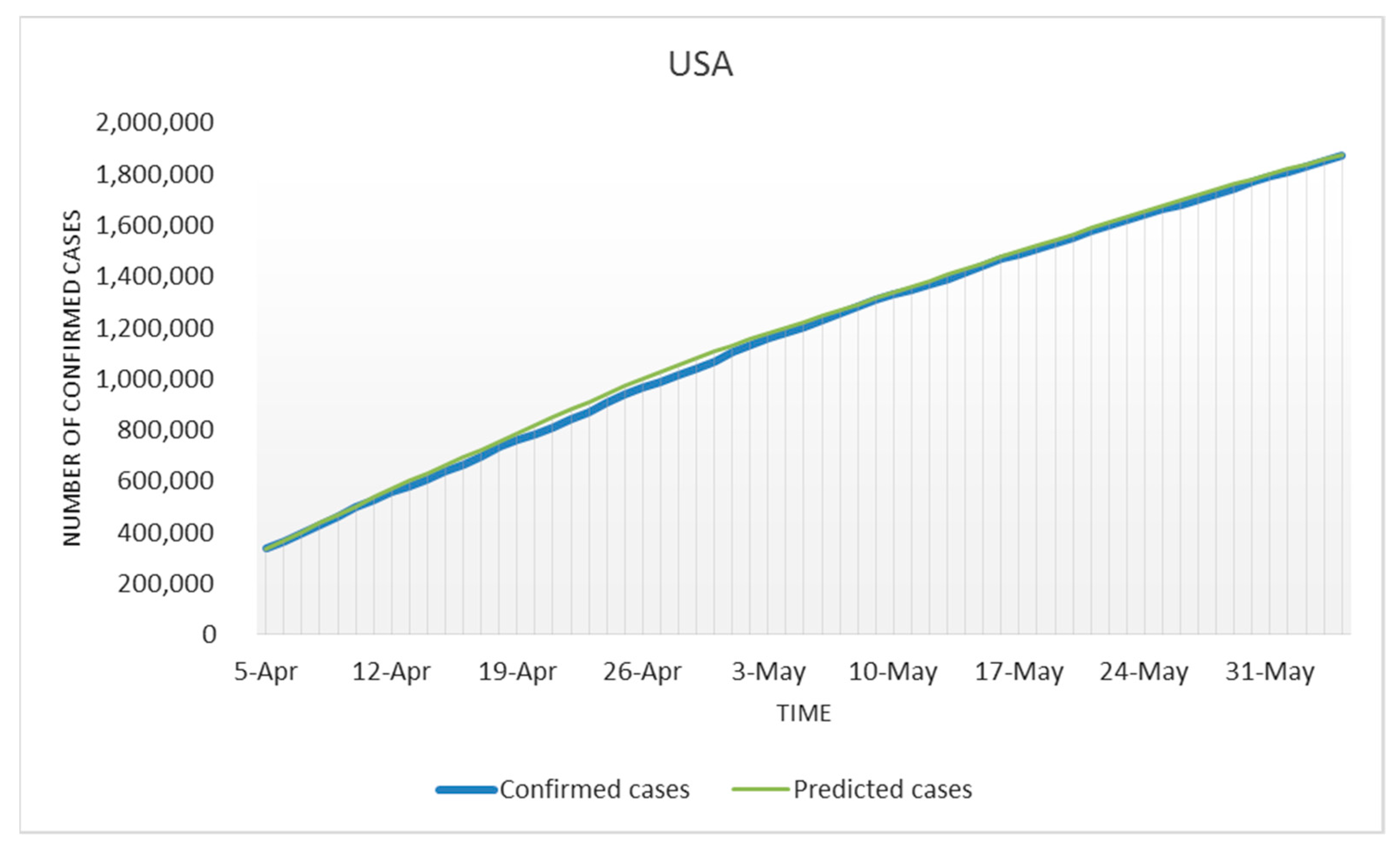
As a result of applying the iterative procedure for generating the $\tilde{I}\left(t\right)$ trajectory for the USA using the CBRR model, the following forecast for the time period 5 April–4 June 2020 was built (Figure 2 and Figure 3). Average deviation of the real-time trajectory of the total number of infected from the one predicted was 0.23%. Standard deviation for the considered time period was 3.9%.

3.2. Modeling for Russia

The epidemic in the Russian Federation (RF), the country-follower, is characterized by a later moment when the same percentage growth rates were reached in comparison with other countries. Based on this fact, when modeling and predicting the dynamics of the epidemic in Russia, we included Italy, Spain, Great Britain, and France as country-predecessors in the ESC chain.

In our first analytical note on the dynamic of the COVID-19 epidemics in Russia, presented online at [27] on 1 May 2020, the question was posed: What could be the estimated date of the epidemic peak in Russia?

As a result of applying the procedure for generating the $\tilde{I}\left(t\right)$ trajectory using the CBRR model for Russia, the following forecast was made on 1 May 2020. It was predicted that the epidemic would reach the peak in the number of active cases not earlier than 16 May 2020. By that time, the total number of confirmed cases could pass the milestone of 160,000.

De facto, the peak of the epidemic in the number of active cases in Russia was reached on May 25, 2020, when 230,996 infected people were registered. In Russia, the total number of 160,000 active cases was surpassed on 5 May 2020, when the total number of confirmed cases was 165,929.

The following forecast was created on 5 May 2020. Given the decrease in the growth rate of the number of active cases in Russia from 9.6% on 22 April 2020 to 6.5% on 5 May 2020, it was believed that, within 2–3 days, the growth rate of the number of active cases would fall below 5% and would reach zero around 18 May 2020. Russia could reach the peak of the epidemic (in terms of the number of active cases) when the growth rate of the total number of infected people would be about 2% and the number of active cases would begin to decline, approximately on 18 May 2020, reaching the level of the total number of 230,000 infected people.

De facto, 217,747 active cases were officially observed on 18 May 2020. The percentage increase in the number of active cases on 20 May 2020 fell below zero (−0.29%). However, later, it began to increase and reached a new negative value of −1.55% on 26 May 2020. Russia reached the first local peak of the epidemic in terms of the number of active cases on 25 May 2020.

The next forecast was presented on 12 May 2020; according to it, considering that the growth rate of the number of active cases in Russia fell below 5% (3.94%) (as predicted on 5 May 2020), the possibility of Russia reaching the peak of the epidemic (in terms of the number of active cases) around 20–21 May 2020 was quite likely. Due to the fact that the absolute value of the increase in the number of infected people over 10 days prior to 12 May 2020 stabilized at around 11,000, a possible option in the next 2–3 days was the change of the number of infected people dynamics to steadily decrease. Thus, it was highly possible that Russia would shortly see the peak of the epidemic in terms of the growth in the number of new cases of the disease (11,656 cases on 11 May 2020). With an average daily growth rate of the number of confirmed cases at 3%, in the period from 12 to 21 May 2020 to May 2020, the total number of infected people by 20–21 May 2020 could reach the level of 305,000.

De facto, Russia indeed reached the peak of the epidemic based on the increment in new cases of the disease on 11 May 2020. The total number of confirmed cases recorded was 308,705 on 20 May and 317,554 on 21 May 2020.

In the forecast dated 16 May 2020, it was noted that with growth dynamics similar to the one at that time, the period of reduction in the percentage increase from 5% to 2–2.5% could take at least 12 days. Russia could reach the peak of the epidemic in terms of the number of active cases on 24 May 2020, with an average daily increase of 3–3.5% (between 12 May and 24 May 2020), reaching the level of the total number of 305,000–350,000 infected individuals.

According to real-world statistical data, the transition from the level of percentage growth of 5% to 2–2.5% took 15 days. The percentage increase crossed the level of 2.5% on 27 May 2020, becoming equal to 2.3%. The total number of confirmed cases on 24 May 2020 was equal to 344,481.

The next forecast was presented on 25 May 2020. It stated that if the slowdown in the growth rate of the number of infected people continued, the projected date of reaching the level of less than 1% should have been adjusted. Under the assumption that the growth rate drops to the level of 2% in 5 days, then the transition from the current level of 2.6% to the level of 1% could take at least 17 days. Therefore, considering the situation at that time, the percentage increase could reach a level of less than 1% on 10–11 June 2020. The local maximum of the number of active cases 230,996 was registered on 25 May 2020. It was necessary to continue monitoring and to check whether the recorded peak was local. At an average rate of the percentage increase in new cases at 1.5% in the period after 25 May 2020, the total number of infected people could increase up to 455,000 on 10 June 2020.

On 31 May 2020, the forecast was adjusted, taking into account the dynamics of the epidemic. The forecast confirmed that the maximum number of active cases registered on 25 May (230,996) most likely only had a local character. Given the fact that between 25 May 2020 and 30 May 2020 the percentage increase in the total number of cases did not fall to the 2% level (as expected in the forecast dated 25 May 2020), the transition from the current level of 2.34% to 1% could take, according to our estimates, not less than 15 days. Therefore, the percentage increase in the total number of confirmed cases could reach a level of less than 1% on 14–15 June 2020 (with an average of 15 days, the daily percentage increase in new cases was 1.5%). The total number of infected people by 10 June 2020 could increase up to 467,000.

In fact, the new local peak of the epidemic in terms of the number of active cases was on 31 May 2020 (234,146 cases). The forecast on the possible locality of the epidemic peak in the number of active cases falling on 25 May 2020, presented in analytical notes dated 25 May 2020 and 31 May 2020, was confirmed. Russia overcame a new local peak of the coronavirus outbreak.

The forecast of 2 June 2020 noted that the transition of the percentage increase in the number of confirmed cases from 5% to 2% had already taken 21 days, which was more than in Spain (8 days), Italy (15 days), Great Britain (18 days), France (11 days), and the USA (14 days). Provided that there was the same rate of growth decline, Russia could drop to the level of 2% in 1–2 days. In that case, by 10–11 June 2020, the total number of infected people could increase up to 491,000. By 20–21 June 2020, the total number of confirmed cases could increase up to 569,000 people.

The transition of the percentage increase in the number of confirmed cases from 5% to 2% ended on 5 June 2020. It took 24 days (instead of the predicted 23 days), that is, the forecast of 2 June 2020, was almost confirmed. The total number of infected people recorded on 10 June 2020, was 493,657, that is, the forecast error was only 0.54%.

On 1 June 2020, a new local peak of the epidemic took shape in terms of the number of active cases—234,146. The previous peak, recorded on 25 May 2020 (230,996), lasted only a week. However, that peak was also surpassed in a week. The number of active cases on 8 June 2020 was 239,999. Thus, in Russia, there was a process of building a chain of several peaks in terms of the number of active cases, which gave food for thought. Based on that information, it was concluded that Russia’s move to a new local peak within the next five days was quite possible.

The following forecast was presented on 10 June 2020. It predicted that, in the event that the percentage increase went down at the same rate, the indicator would reach 1% in about 20 days, on 30 June 2020. The total number of infected people according to the statistics as of 30 June 2020, could reach 655,000. By 20 May 2020, the value of this indicator was about 582,000, which was 2.3 % more than the forecast of 2 June 2020.

On 15 June 2020, the forecast on the possibility of Russia reaching a new epidemic peak concerning the number of active cases from 11 to 15 June presented in a note dated 10 June 2020 was confirmed. On 15 June, the highest value for the entire epidemic was recorded—245,580 active cases. Thus, the supposedly third local peak was registered.

Simulation Results for Russia

The result of the experiment on the use of the CBRR model for predicting the trajectory of the percentage increase rate and the absolute number of confirmed cases during the time period from 20 April to 31 July 2020 is shown in the graphs (Figure 4 and Figure 5). The predicted dynamics is compared with the actual dynamics provided in the official statistical reports. The average deviation of the predicted trajectory of the number of confirmed cases from the actual one in the time period from 20 April 2020 to 31 July 2020 is 0.28%. The standard deviation for the considered time period was 3.7%.

4. Discussion

The results of the study exceeded our expectations. The hypothesis about the effect of the dynamics of percentage growth in the ESC countries on the future dynamics of the total number of confirmed cases in the country-followers was confirmed. That allowed us to make 2–3 week forecasts with three predicting intervals for the epidemic development in Russia, as well as in the USA. Similar modeling could be performed for other countries for which ESCs with a sufficient lead time in terms of percentage growth dynamics would be formed.

References

1. Layne, S.P.; Hyman, J.M.; Morens, D.M.; Taubenberger, J.K. New coronavirus outbreak: Framing questions for pandemic prevention. Sci. Transl. Med. 2020, 12, eabb1469. [Google Scholar] [CrossRef] [PubMed] [Green Version]
2. The Novel Coronavirus Pneumonia Emergency Response Epidemiology Team. Vital surveillances: The epidemiological characteristics of an outbreak of 2019 novel coronavirus diseases (COVID-19)-China 2020. China CDC Wkly. 2020, 2, 113–122. [Google Scholar] [CrossRef]
3. Wu, J.T.; Leung, K.; Leung, G.M. Nowcasting and forecasting the potential domestic and international spread of the 2019-nCoV outbreak originating in Wuhan, China: A modelling study. Lancet 2020, 395, 689–697. [Google Scholar] [CrossRef] [Green Version]
4. MIDAS Coordination Center. Models of Infectious Disease Agent Study (University of Pittsburgh, 2020). Available online: https://midasnetwork.us/ (accessed on 23 June 2020).
5. Kondratyev, M.A. Forecasting methods and models of disease spread. Comput. Res. Model. 2013, 5, 863–882. [Google Scholar] [CrossRef]
6. Mandal, M.; Jana, S.; Nandi, S.; Khatua, A.; Adak, S.; Kar, T.K. A model based study on the dynamics of COVID-19: Prediction and control. Chaos Solitons Fractals 2020, 136, 109889. [Google Scholar] [CrossRef] [PubMed]
7. Bekirosab, S.; Kouloumpou, D. SBDiEM: A new mathematical model of infectious disease dynamics. Chaos Solitons Fractals 2020, 136, 109828. [Google Scholar] [CrossRef]
8. Barmparis, G.D.; Tsironis, G.P. Estimating the infection horizon of COVID-19 in eight countries with a data-driven approach. Chaos Solitons Fractals 2020, 135, 109842. [Google Scholar] [CrossRef]
9. Kissler, S.M.; Tedijanto, C.; Goldstein, E.; Grad, Y.H.; Lipsitch, M. Projecting the transmission dynamics of SARS-CoV-2 through the postpandemic period. Science 2020, 368, 860–868. [Google Scholar] [CrossRef]
10. Fanelli, D.; Piazza, F. Analysis and forecast of COVID-19 spreading in China, Italy and France. Chaos Solitons Fractals 2020, 134, 109761. [Google Scholar] [CrossRef]
11. López, L.; Rodó, X. The end of social confinement and COVID-19 re-emergence risk. Nat. Hum. Behav. 2020, 4, 746–755. [Google Scholar] [CrossRef]
12. Otunuga, O.M.; Ogunsolu, M.O. Qualitative analysis of a stochastic SEITR epidemic model with multiple stages of infection and treatment. Infect. Dis. Model. 2020, 5, 61–90. [Google Scholar] [CrossRef] [PubMed]
13. Cooper, I.; Mondal, A.; Antonopoulos, C.G. A SIR model assumption for the spread of COVID-19 in different communities. Chaos Solitons Fractals 2020, 139, 110057. [Google Scholar] [CrossRef] [PubMed]
14. Singh, R.K.; Rani, M.; Bhagavathula, A.S.; Sah, R.; Rodriguez-Morales, A.J.; Kalita, H.; Nanda, C.; Sharma, S.; Sharma, Y.D.; Rabaan, A.A.; et al. Prediction of the COVID-19 pandemic for the top 15 affected countries: Advanced autoregressive integrated moving average (ARIMA) model. JMIR Public Health Surveill. 2020, 6, e19115. [Google Scholar] [CrossRef]
15. Sharma, V.K.; Nigam, U. Modeling and forecasting of Covid-19 growth curve in India. MedRxiv 2020. [Google Scholar] [CrossRef]
16. Zhang, T.; Ma, Y.; Xiao, X.; Lin, Y.; Zhang, X.; Yin, F.; Li, X. Dynamic bayesian network in infectious diseases surveillance: A simulation study. Sci. Rep. 2019, 9, 10376. [Google Scholar] [CrossRef]
17. Akhtar, M.; Kraemer, M.U.G.; Gardner, L.M. A dynamic neural network model for predicting risk of Zika in real time. BMC Med. 2019, 17, 171. [Google Scholar] [CrossRef] [Green Version]
18. Schmidt, R.; Waligora, T. Influenza forecast: Case-based reasoning or statistics? In Lecture Notes in Computer Science, Proceedings of the 11th International Conference on Knowledge-Based Intelligent Information and Engineering Systems, Vietri sul Mare, Italy, 12–14 September 2007; Apolloni, B., Howlett, R.J., Jain, L., Eds.; Springer: Berlin/Heidelberg, Germany, 2007; Volume 4692, pp. 287–294. [Google Scholar] [CrossRef]
19. Viboud, C.; Boelle, P.Y.; Carrat, F.; Valleron, A.J.; Flahault, A. Prediction of the spread of influenza epidemics by the method of analogues. Am. J. Epidemiol. 2003, 158, 996–1006. [Google Scholar] [CrossRef] [Green Version]
20. Relich, M.; Pawlewski, P. A case-based reasoning approach to cost estimation of new product development. Neurocomputing 2018, 272, 40–45. [Google Scholar] [CrossRef]
21. Kaedi, M.; Ghasem-Aghaee, N. Improving case-based reasoning in solving optimization problems using Bayesian optimization algorithm. Intell. Data Anal. 2012, 16, 199–210. [Google Scholar] [CrossRef]
22. Teles, P. Predicting the evolution of SARS-Covid-2 in portugal using an adapted SIR model previously used in south Korea for the MERS outbreak. MedRxiv 2020. [Google Scholar] [CrossRef]
23. COVID-19 Dashboard by the Center for Systems Science and Engineering (CSSE) at Johns Hopkins University. Available online: https://coronavirus.jhu.edu/map.html (accessed on 4 August 2020).
24. Popkov, Y.; Popkov, A.; Dubnov, Y.; Solomatine, D. Entropy-randomized forecasting of stochastic dynamic regression models. Mathematics 2020, 8, 1119. [Google Scholar] [CrossRef]
25. Zakharov, V.; Balykina, Y. Predicting the dynamics of the coronavirus (COVID-19) epidemic based on the case-based reasoning approach. Appl. Math. Comput. Sci. Control Process. 2020, 3, 249–259. [Google Scholar]
26. Coronavirus Epidemic in Russia. Dynamics Modeling and Forecasting. Available online: http://hdl.handle.net/11701/18124 (accessed on 7 September 2020).
27. The Coronavirus Epidemic in Russia. Intelligent Logistics Center Analytical Notes. Available online: http://www.apmath.spbu.ru/cil/ (accessed on 20 September 2020).
Figure 1. Steps for constructing the forecast trajectory of the coronavirus epidemic dynamics based on the Case-Based Rate Reasoning (CBRR) approach.
Mathematics 08 01727 g001
Figure 2. Total number of confirmed cases in the USA (real-world data and model forecast).
Mathematics 08 01727 g002
Figure 3. Growth rate over the considered time period in the USA (real-world data and model forecast). Red dotted lines correspond to the growth rates of 5% and 2%.
Mathematics 08 01727 g003
Figure 4. Total number of confirmed cases in the Russian Federation (RF) (real-world data and model forecast).
Mathematics 08 01727 g004
Figure 5. Growth rate over the considered time period in the RF (real-world data and model forecast). Red dotted lines correspond to the growth rates of 5% and 2%.
Mathematics 08 01727 g005