Abstract
The distributed material warehouse is the crucial link in the process of modern enterprise construction, and the goal of the enterprise is to save the cost of material distribution and reduce the time of distribution. In order to obtain the optimal ordering and allocation scheme, firstly, a distributed inventory system consisting of an ordering centre, a material coordination centre and n material warehouses are considered, and the cost model of ordering and allocation of the distributed material warehouse is established. Next, the safety stock and the ordering point of the distributed material warehouse are solved. Then the improved genetic algorithm-simulated annealing algorithm (IGA-SA) is used to solve the optimization of the distributed material warehouse. Finally, the application example is given. The results show that the IGA-SA algorithm can effectively reduce inventory cost and improve inventory utilization.
1. Introduction
In the process of module construction in traditional enterprises, the material management is mostly centred on the material warehouse, and each inventory centre has a high degree of autonomy to deliver materials directly to the construction centre. The material management department of the construction enterprise orders materials from the ordering centre and distributes them to each material warehouse, which makes decisions and operates independently [1]. This kind of inventory management method cannot consider the overall interests of the construction enterprise, and the lack of cooperation between the material warehouses leads to low construction efficiency and increasing the cost of material storage. Besides, it is easy to generate material accumulation. In order to realize the organic integration of each material warehouse, the concept of coordination centre is put forward to manage the material distributed system [2].
The so-called distributed inventory management refers to the inventory management system composed of multiple warehouses based on a coordination centre [3]. In terms of space, warehouses can be located in the same area or planned in different areas. However, most manufacturing enterprises, in order to facilitate production, set up the warehouses near the construction centre, i.e., production base.
At present, the research on the distributed material warehouse at home and abroad mainly focuses on the establishment of the distributed inventory model and the coordination of each storage point, and the analysis of the algorithm for solving the model is relatively less. The single algorithm is the main one. Concerning the establishment of the distributed inventory model, Literature [4] innovatively puts forward a cross-node inventory collaborative solution. It establishes a short-term demand prediction calculation model, which ensures the effectiveness of the inventory control scheme by collecting inventory data in real-time. The genetic algorithm used in the literature needs a large amount of data to learn, and its efficiency is low. Moreover, the solving method of genetic algorithm is more suitable for the robust data model, and the solving accuracy of the actual model corresponding to the constantly fluctuating demand is poor. The literature [5] puts forward a new type of distributed inventory system based on system dynamics. The purpose is to coordinate and manage the nodes distributed in different positions and realize the optimal allocation of resources. The idea of establishing the system model in this paper provides some ideas, but a new set of matching algorithm is needed which can solve the model of the literature system to adapt the real-time change of inventory demand. The model algorithm in this paper less universal and only suitable for solving specific problems. The literature [6] mainly discusses different strategies of storage point scheduling, proposes selfish allocation strategy, cooperative allocation strategy and mixed allocation strategy by establishing allocation model, and then analyzes and compares the optimal results. However, this paper does not explain the relevant conclusions well, and the proposed hybrid strategy optimal solution lacks further discussion on the influence of multiple strategy weights. The literature [7] puts forward an alliance ordering strategy, which extends the single warehouse control model to the distributed inventory model with deterministic discrete demand, and uses a genetic algorithm to solve the optimal solution. This model is suitable for large-scale production chain, but it is not universal because of the lack of discussion on specific single warehouse point in model transformation. The literature [8] combined with spare parts inventory system model in a distributed environment, proposed a new distributed inventory model based on Web, which mainly integrated real-time information into the calculation model to optimize the inventory of spare parts system and reduce costs. However, this method lacks the consideration of the computational efficiency of the algorithm model, and large-scale information interaction will increase the time cost in the process. The literature [9] discusses the continuous review inventory model with fuzzy service level constraints and fuzzy random parameters and establishes the mathematical model of the fuzzy random environment. The model in this paper takes into account the actual environmental impact, and adds a large number of parameters into the solution, which requires a large amount of calculation. Moreover, a large number of influence parameters need to be further optimized, so the calculation efficiency is not high. The literature [10] puts forward a new inventory management method, which uses the triangular distribution of unit time demand and lead time demand, and a method of estimating the probability density function of unknown lead time demand distribution. It uses this method to establish an inventory model suitable for new products by optimizing related costs. In this paper, the managers in the process are added to the whole analysis process, but some flexibility analysis of the (Q, r) model proposed in the paper is lacking, and the applicability research in other situations need further explanation. The literature [11] puts forward a new structure of multi-frequency distributed demand and fixed-cost inventory model, and this paper explains the problem of local minimum boundedness which is lacking in existing inventory theory. It provides some reference for the model derivation and theoretical calculation in this paper, but the theory lacks a more sufficient explanation for the practical example.
The above literatures show that the research on the actual material management model has been very sufficient, but there are few researches on the optimization of solving the model algorithm, and more on the specific solving algorithm for the specific model system. The applicability is not strong, and there is a lack of attention to the efficiency problem of solving the actual model with a lot of parameters. Based on the distributed inventory control model, this paper makes an improved solution algorithm based on IGA-SA to solve the optimal ordering and distribution scheme for the material ordering model and distribution cost model based on practical problems. The research contents of this paper are as follows:
- (1)
- The ordering and transfer cost model of material distributed system considering random material demand, lead time of ordering center and discount of ordering is established. Compared with the previous models, this model is more in line with the actual management requirements
- (2)
- The improved algorithm based on genetic and simulated annealing is adopted, and IGA-SA algorithm is used to solve the best material ordering scheme and distribution scheme.
- (3)
- The programming solution simulates a real example to verify the effectiveness of the proposed algorithm in this paper, obtains the optimal configuration scheme, and compares the proposed method with the traditional one, proving that the proposed method is superior to the traditional one.
2. Establishment and Analysis of Cost Model
2.1. Conditional Hypothesis
The material distribution system studied in this paper is composed of a material coordination centre and multiple storage points. Among them, the material coordination centre mainly plays the role of managing distributed material system information, coordinating the material inventory information of each storage point and interacting the corresponding information with the reservation centre, and making the reservation or transfer operation in time. The concrete operation mechanism can be divided into two parts. First, the reservation management, which firstly provides the shortage information by each warehouse, then the material coordination centre judges whether the reservation operation is needed, and interacts with the reservation centre for the detailed information of the shortage of materials, finally, the reservation centre provides the materials to each warehouse. The second is allocation management, in which the shortage of information is directly provided by each warehouse and analyzed and processed by the material coordination centre. According to the information such as the quantity and time required by each warehouse, the inventory situation of each warehouse, etc., make a transfer plan, and other warehouses provide materials to the required warehouse. This material allocation scheme can maintain a specific inventory at each storage point, ensure that there is no shortage of materials and no surplus of materials, effectively reduce the storage cost of materials, and improve the construction efficiency of large modules. The assumptions are as follows [12]:
- (1)
- This material distributed system uses the method of regularly checking the inventory of each storage point, unifying the ordering, and using the (R, Q) ordering strategy [13], that is, each storage point continuously checks its material inventory. When the total material inventory level of all storage points is lower than the ordering point R, the material coordination centre issues the ordering request to the ordering centre, and orders the materials of Q units.
- (2)
- Supposing that the material demand Dit of any storage point i () obeys the normal distribution [14], and the material demand of each storage point every day is independent. Therefore, in t (unit: day) days, the material demand Dit of the ith storage point obeys the normal distribution .
Model optimization objective: under the premise of limited material inventory level of each storage point, with time t as the cycle and given service level y, the material inventory optimization scheme of each storage point is determined to minimize the inventory cost and material distribution cost, to achieve the purpose of cost optimization.
2.2. Variable Provision
In the process of building the distributed centralized control model of this material, multiple variables are involved. In order to facilitate searching and model building, all variables are listed in Table 1.

Table 1.
Definition of variables.
2.3. Ordering Cost Model
The centralized ordering cost of the material distributed system includes warehouse keeping cost, shortage cost, ordering cost and transportation cost. Each cost will be calculated separately below.
(1) Warehouse keeping cost C1. The warehouse keeping cost is related to the number of materials stored in the storage point, including all expenses of materials in the storage process of the storage point, such as the funds occupied by materials, the storage fees of materials, the user fees of the storage point, taxes and security funds. In the calculation of warehouse keeping cost, some costs are allocated to each material in a particular proportion, such as the salary of warehouse management personnel and the loss of the materials during storage, and the storage cost of materials is determined reasonably and accurately as possible. Warehouse keeping cost C1 can be calculated by the following Formula:
(2) Shortage cost C2. Shortage cost refers to the cost of production and construction delay caused by the lack of a specific material at one or more storage points at the same time. In general, when one storage point is short of materials, there will be other storage points to supplement, so it also involves the transportation cost of materials. The shortage cost C2 can be calculated by the following Formula:
(3) Ordering cost C3. The ordering cost is the cost of ordering related materials from the ordering centre due to the lack of materials during the construction process. It is mainly divided into two parts. One is the fixed cost generated each time the materials are ordered. This part of the cost is not related to the ordering quantity. The other is the cost of purchasing materials. This model considers materials a discount when a large number of purchases are made, and this part of the cost is related to the number of materials purchased. The following Formula can calculate the ordering cost C3:
(4) Transportation cost C4. C4 is the transportation cost generated by allocating materials to each storage point when materials are ordered. Therefore, the transportation cost is counted into the storage management cost here. Transportation cost C4 can be calculated by the following Formula:
When calculating the total cost Z1i of materials ordered by storage point i from the ordering centre in t time, it is necessary to include the labour cost CPit of each time the materials are put into storage and the cost CIt of materials input to storage point i, and set:
Then the total cost Z1i generated by storage point i when ordering materials from the ordering centre within t time is as follows:
In Formulas (3)–(6), define:
In t time, when the material mentioned above-distributed system orders materials centrally, the total order cost Z2 generated by the whole storage system is as follows:
When ordering materials at each storage point, the number of materials ordered shall be less than the maximum storage capacity of the storage point, and also less than the maximum supply capacity of the ordering centre. Besides, in order to ensure that the inventory number of each storage point meets the actual demand, the sum of the transferred-in material quantity of storage point i and the remaining material quantity of storage point i before transfer should be higher than the critical ordering point of the current storage point. Therefore, the constraints of the model are as follows:
2.4. Allocation Cost Model
In the process of allocation, storage points transfer to each other. First, determine the optimal stock of each storage point, reasonably allocate the material resources of each storage point, and reduce the storage cost of materials. The total cost of material allocation includes storage and maintenance cost, shortage cost, allocation transportation cost, processing cost during allocation, material issue and receipt processing cost, etc. The total cost of the allocation cost model can be obtained by referring to the ordering cost model. The total cost Z3i generated by warehouse i when transferring materials within t time is as follows:
In this formula, C6 is the storage and maintenance cost, C7 is the shortage cost, C8 is the transportation cost of the material, C9 refers to the handling cost of material allocation, the cost of material issue and receipt, and the labour cost required for material allocation. Qijt represents the material quantity transferred between storage point i and storage point j, the positive value represents the material quantity transferred from storage point i to storage point j, and a negative value is an opposite. Also, define:
On this basis, the allocation cost model of storage point i is as follows:
In the t time, the total allocation cost Z4 generated by the whole storage system is as follows:
When each storage point is transferred, the number of materials transferred to the warehouse shall be less than the maximum storage capacity of the storage point. At the same time, the number of materials transferred to the storage point after allocation shall be higher than the ordering point. Also, the sum of the transferred number of storage point I and the quantity of materials in storage point i before ordering shall be higher than the ordering point of the current storage point. Therefore, the constraints of the model are as follows:
2.5. Analysis of Cost Model
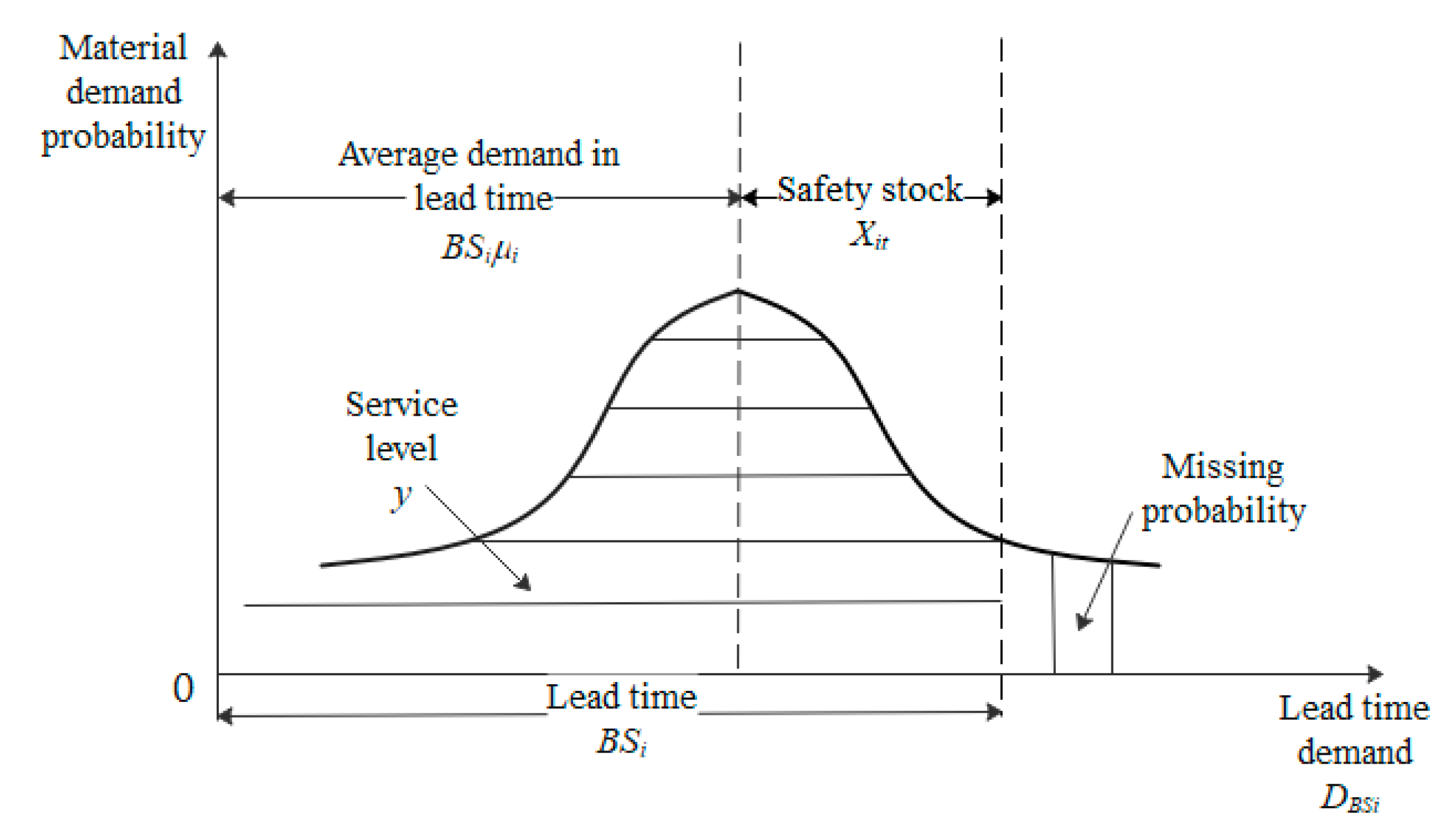
According to the assumptions of the cost model of the material distribution system, the material demand Di of any storage point i () is subject to the normal distribution , and the material demand of each storage point is independent every day. Therefore, within the material supply lead time BSi, the material demand DBSi of storage point i is subject to the normal distribution . As shown in Figure 1.
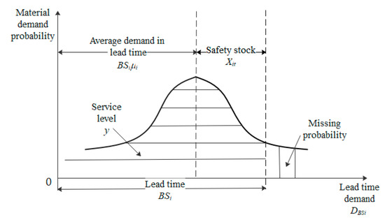
Figure 1.
Probability distribution of material demand.
In Figure 1, the horizontal line on the left represents the situation without material shortage, and the vertical line on the right represents the situation with the material shortage. According to the image characteristics of the normal distribution function, the area of the shadow part represents the probability of a corresponding situation [15].
Take the probability that the material demand DBSi within the lead time BSi does not exceed the Rit of the order point as the service level y, then:
because of the normal distribution of material demand DBSi, the standard normal distribution can be obtained:
in this formula, is the random variable of the standard normal distribution, and 1-y is the quantile of the standard normal distribution [16].
According to the above formula:
Then the ordering point of the storage point can be obtained as follows:
According to the relationship between the order point and safety stock:
It can be seen that the safety stock is:
3. Improvement of the Genetic Simulated Annealing Algorithm
The calculation speed of the genetic algorithm is fast, but it is easy to fall into the local extremum [17], while the convergence speed of simulated annealing algorithm is slow, but it is not easy to fall into the local extremum [18]. Therefore, some scholars put forward the genetic simulated annealing algorithm by combining the two algorithms [19]. Genetic simulated annealing algorithm is based on the idea of combination. It can not only keep the advantage of fast computing speed of the genetic algorithm but also integrate the advantage of strong local search ability of simulated annealing algorithm to improve the overall computing effect. This section will improve the genetic simulated annealing algorithm, propose IGA-SA algorithm, and analyze the main steps of the algorithm to solve the model.
3.1. Improved Adaptive Crossover and Mutation Probability
The crossover probability Pc and mutation probability Pm in the genetic algorithm are the key factors affecting its performance [20]. Among them, the crossover probability determines the diversity of the population, and the mutation probability determines whether it can jump out of the local extremum, so choosing the appropriate crossover and mutation probability can get the optimal solution of the model faster. However, in the traditional genetic algorithm, the probability of crossover and mutation is constant, so it is difficult to ensure the optimal in the actual calculation. In this section, according to the population adaptability, the adaptive crossover and mutation probability are improved as follows:
In this formula, is the average value of fitness function, is the maximum value of fitness function, and , is the adaptive parameter.
3.2. Improved Fusion Metropolis Criterion
Metropolis criterion was put forward by Metropolis in 1953 and described by the process of substantial reaching thermal equilibrium at a constant temperature [21]. The physical system tends to be in a state of lower energy, while thermal motion prevents it from falling into the lowest state accurately. This phenomenon focuses on those states that have essential contributions when sampling by Metropolis criterion, and then better results can be obtained quickly.
The convergence speed of traditional simulated annealing algorithm is slow, and the modification of individuals by standard Metropolis criterion can only be divided into two cases, that is, to accept new individuals or to retain old ones, which makes the diversity of population insufficient [22]. In this section, we will propose the improved fusion Metropolis criterion, and modify the individual population in different situations to ensure the diversity of the population. The steps to improve the metropolis criteria for fusion are as follows:
- (1)
- Define the new solution acceptance probability P:In this formula, k is Boltzmann constant, is a fitness function value of the individual in new species group, and is a fitness function value of the individual in geriatric populations.
- (2)
- When the individual fitness function value in the new solution is larger than that in the old solution, the new individual is accepted as the basis of the next iteration.
- (3)
- When the individual fitness function value in the new solution is less than that in the old solution, the gene of the new individual will be interchanged with the gene of other positions with a probability of 0.01. The individual in the new solution will be accepted with a probability of P, and the other individuals in the old solution will be accepted.
The improved fusion Metropolis criterion can not only generate new individuals through gene exchange in individuals to improve the performance of individuals but also improve the diversity of individuals through probability method to improve the algorithm’s solving ability.
4. Numerical Example
4.1. Example Description
The necessary information of each storage point for a specific material is shown in Table 2.
Table 2.
The necessary information of each storage point for a specific material.
The expenses incurred in ordering or transferring materials at each storage point are shown in Table 3. When the storage point is short of materials and needs to order materials, the discount will be generated according to the number of materials ordered. The specific discount information is shown in Table 4.
Table 3.
Cost of each storage point.
Table 4.
Discount price list when ordering materials.
4.2. Solution and Analysis of the Ordering Process
According to formulas (19) and (20), the order point and safety stock of storage point 1–4 can be obtained. When y = 95%, the safety factor 1-y = 1.65. Thus, it can be calculated that the safety stock V1 = 4, V2 = 6, V3 = 5, V4 = 5, the order point R1 = 34, R2 = 66, R3 = 26, R4 = 37, and the total order point is 163. According to Table 2, the total initial inventory of the four storage points is 94. Since the total ordering point is 163, which is greater than the total initial inventory of 94, so it is necessary to order.
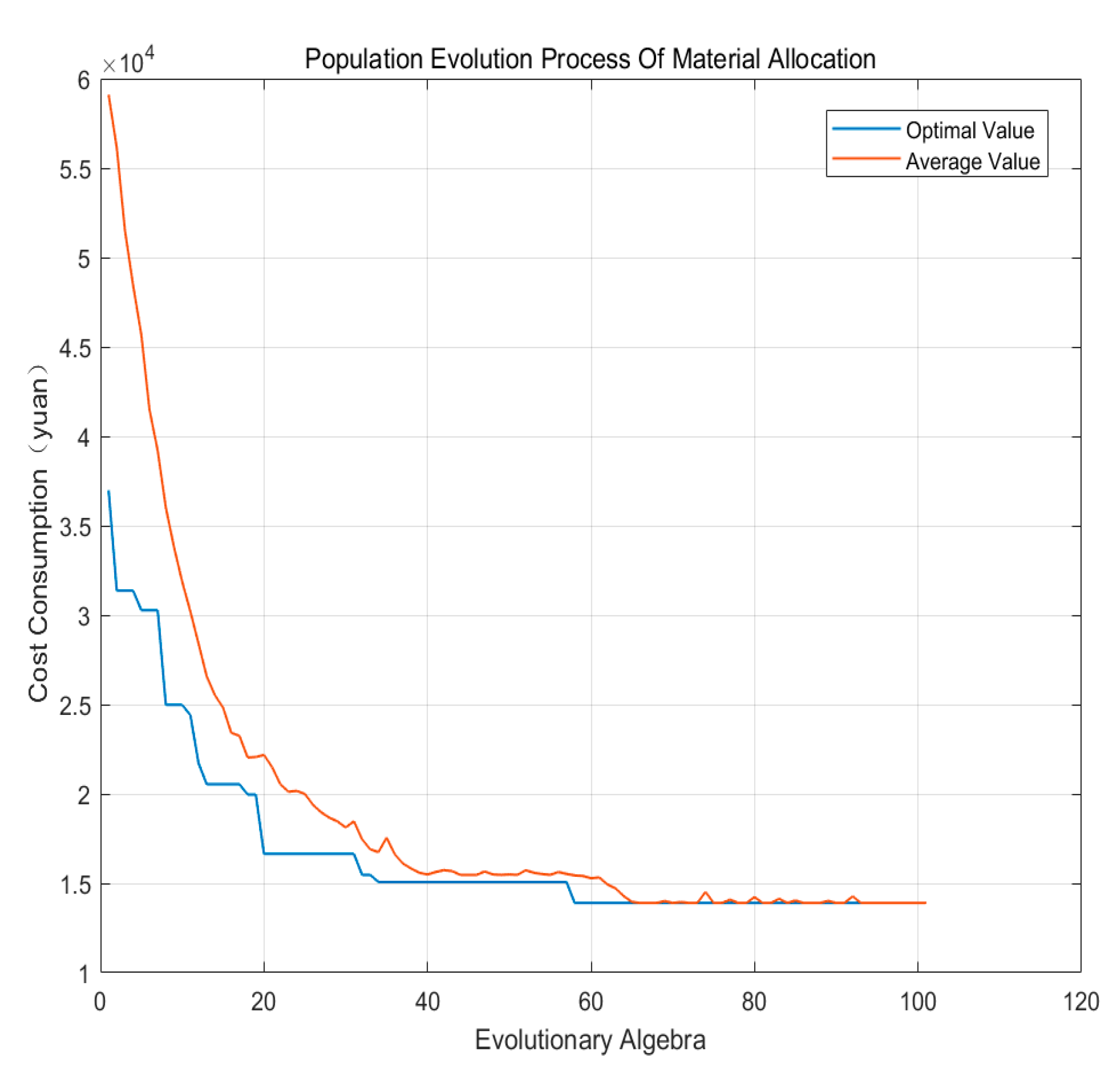
Using MATLAB to compile IGA-SA algorithm program to solve the optimal order quantity and the corresponding cost of the order model. With the iteration, the individuals with relatively low fitness function value in the population are eliminated, and the individuals with high fitness remain. They are concentrated near the optimal individuals so that the optimal solution or close to the optimal solution can be determined. The evolution process of the population is shown in Figure 2. The two curves in the figure, respectively represent the minimum value and average value of the cost function in the process of distributed material inventory ordering. It can be seen that when the population evolves to 50 generations, the two curves almost coincide and tend to converge at this time.

Figure 2.
The change of the optimal value and average value of the ordering cost.
The optimal solution can be obtained in the 50th generation by outputting the optimal result after 100 iterations. At this time, the ordering scheme and cost of material distributed system are shown in Table 5.
Table 5.
Ordering scheme and cost of material distributed system.
If according to the original ordering strategy of the enterprise, each storage point separately orders materials. According to each storage point to meet their minimum inventory demand, we can get the best order quantity and make the total order cost the lowest. At this time, the ordering plan of the four storage points is shown in Table 6.
Table 6.
Original ordering scheme and cost.
The comparison between the two schemes is shown in Table 7. Compared with the traditional scheme, the centralized ordering scheme reduced the order quantity by 18.21%, totaling 53 item, and the total ordering cost decreased by 17.22%, totaling 10,705 yuan. It can be seen that the scheme of centralized ordering reduces the total inventory of materials, improves the utilization ratio of inventory and reduces the total cost of ordering. At this time, the centralized ordering scheme is better.
Table 7.
Comparison between centralized and decentralized orders.
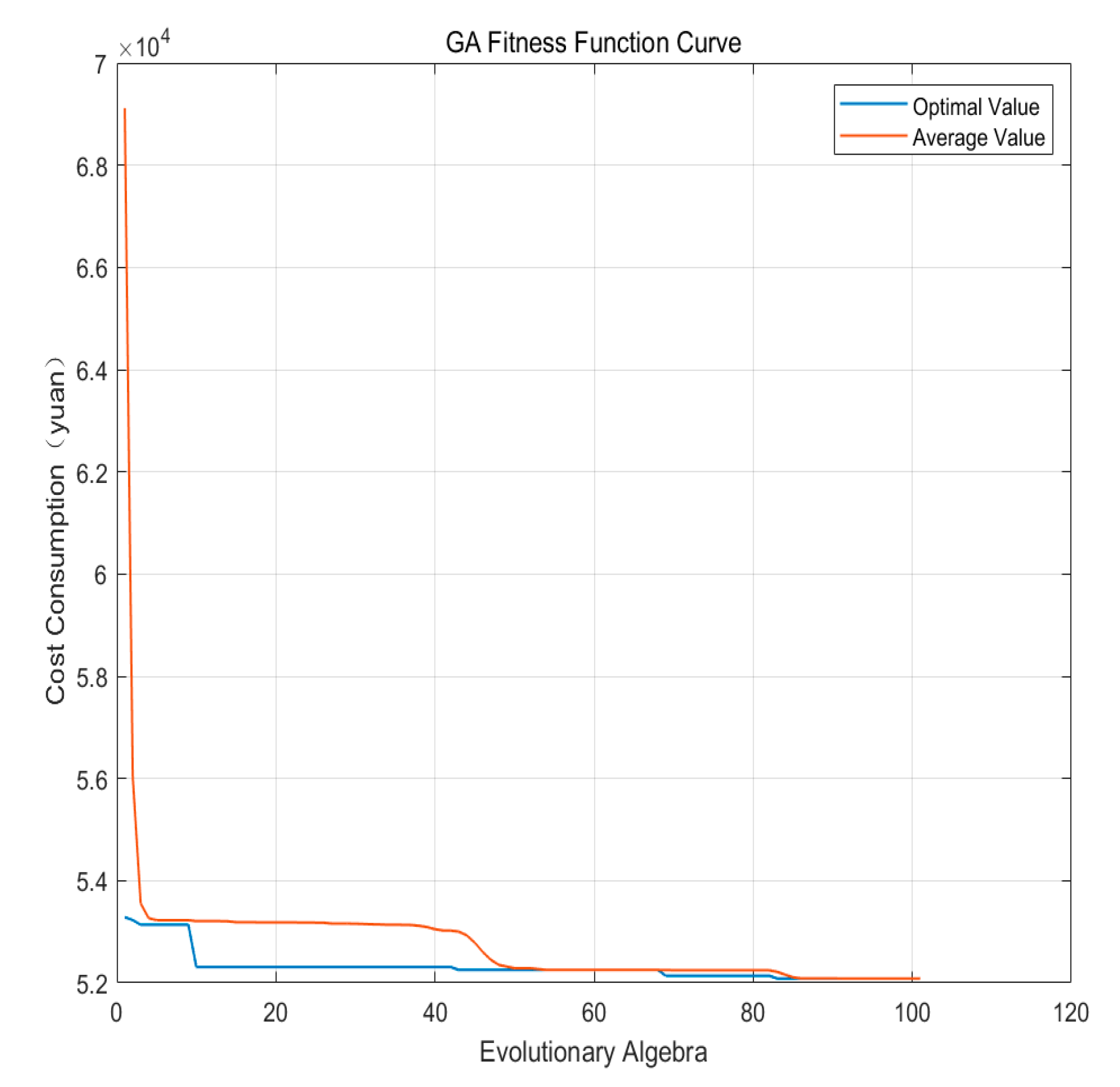
GA is the abbreviation of genetic algorithm. In order to verify the effectiveness of algorithm proposed in this paper, GA and IGA-SA are used to calculate the above examples. The evolution process of the population is shown in Figure 3 and Figure 4, respectively.
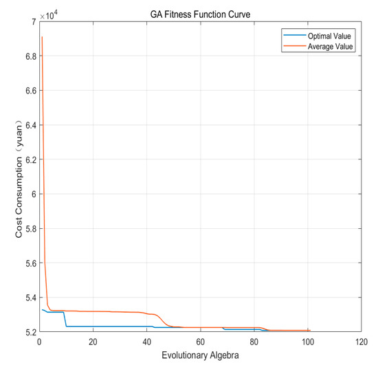
Figure 3.
Population evolution process solved by GA.
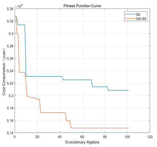
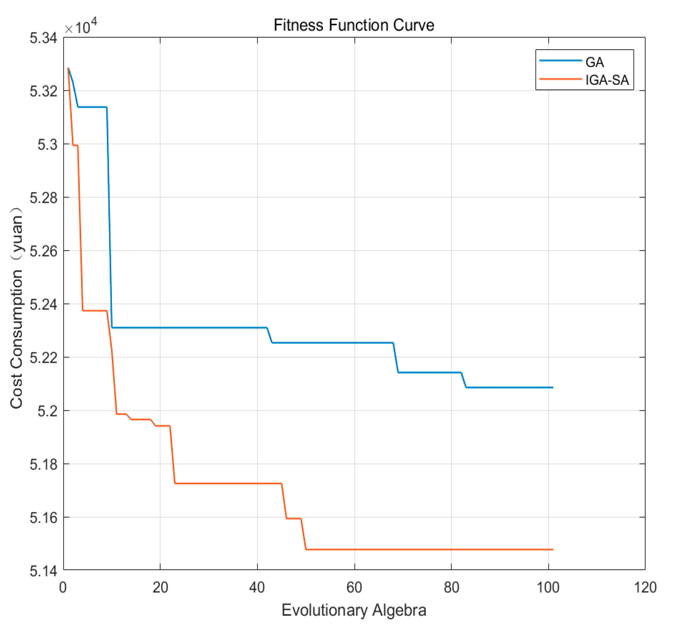
Figure 4.
Comparison results of the two algorithms.
Compare the above results obtained by different algorithms, as shown in Table 8.
Table 8.
Algorithm comparison.
It can be seen from Table 8 that the iteration time of IGA-SA is 33 times less than GA, and the total optimal ordering cost is reduced by 608 yuan. We can concluded that the simulated annealing process can effectively avoid GA falling into local extremum. The IGA-SA algorithm proposed in this paper can not only be further improved in evolutionary algebra but also get better model solution than GA algorithm.
4.3. Solution and Analysis of Allocation Process
When the initial inventory of each storage point is shown in Table 9, it can be seen that at this time, the total initial stock of materials in each storage point is 163, while the total order point is 245, so the initial stock is larger than the order point, so there is no need to order. However, since the initial inventory of storage points 2 and 4 are smaller than their ordering points, the allocation operation is adopted.
Table 9.
Initial inventory of each storage point.
The distance between the four storage points is shown in Table 10.
Table 10.
Allocation distance between four storage points (unit: km).
The IGA-SA algorithm is still used to solve the optimal allocation scheme and allocation cost of the allocation model. The evolution process of the population is shown in Figure 5. It can be seen that when the population evolves to 60 generations. The optimal value curve tends to converge, and the allocation cost is the lowest at this time. The best allocation scheme and allocation cost of the distributed material system are shown in Table 11.
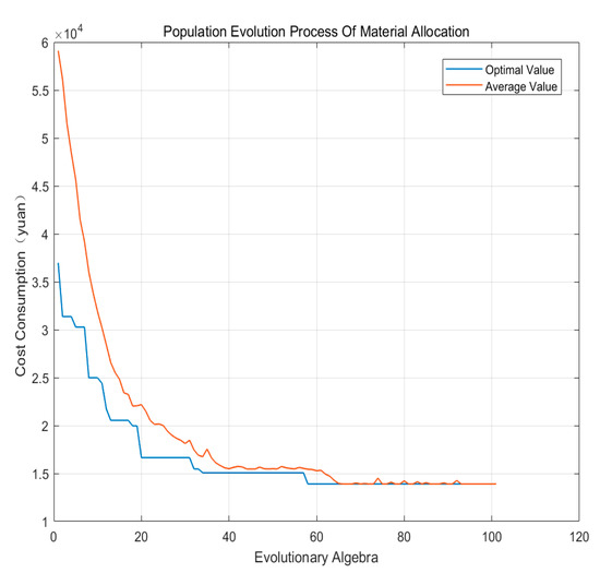
Figure 5.
The change of the optimal value and average value of the allocation cost.
Table 11.
The best allocation scheme and cost of the distributed material system.
If the centralized feeding scheme is still adopted at this time, the population evolution process is shown in Figure 6. It can be seen that when the population evolves to 35 generations, the two curves almost coincide and tend to converge at this time.
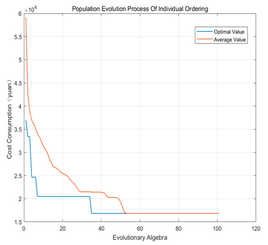
Figure 6.
The change of the optimal value and average value of the ordering cost.
By outputting the optimal result after 100 iterations of the population, the centralized ordering scheme of the material distribution system can be obtained, as shown in Table 12.
Table 12.
Centralized ordering plan and cost.
It can be seen from Table 11 and Table 12 that if the centralized order scheme is adopted, the order quantity of all storage points is Q1 = 66, and the total ordering cost is 16,819 yuan; if the mutual allocation scheme is adopted, the total allocation quantity of all storage points is 53, and the total allocation cost is 13,899.7 yuan.
Through the above comparison, it can be concluded that: (1) When the total initial inventory of materials in each storage point does not reach the total ordering point, the strategy of transferring materials among storage points can reduce the overall inventory level of materials in enterprises and effectively avoid the problem of material backlog caused by traditional methods; (2) This strategy greatly reduces the occupation of material funds, that is, it increases the liquidity of enterprises and optimizes the overall level of material inventory.
Through the above calculation and analysis of the ordering cost model and transfer cost model of the material distributed system, we can know that: (1) when the total initial inventory of materials at each storage point does not reach the total ordering point, the unified ordering scheme has more advantages than the individual ordering at each storage point; (2) When the total initial stock of materials in each warehouse exceeds the total ordering point, but the initial stock of materials in some warehouses does not reach its ordering point, it is more advantageous to adopt the scheme of mutual transfer between warehouses than to order materials separately in shortage warehouses. Besides, the IGA-SA algorithm proposed in this paper is compared with GA algorithm, and the validity of the IGA-SA algorithm is verified.
5. Discussion
In this paper, the improved IGA-SA algorithm is used to solve the optimal cost based on the material distribution model. Through the data, we can see that the convergence speed and the cost of this method are greatly optimized compared with the traditional algorithm. And there are many researches on distributed material management, such as the establishment and solution analysis of multi-coordination center model, the establishment and analysis of evaluation system model and scheme decision model, and the retrieval and storage of open source database information suitable for distributed material management.
6. Conclusions
The key to the distributed material warehouse system is inventory optimization. Based on the IGA-SA algorithm, this paper studies the centralized ordering and allocation scheme of the distributed material warehouse. With fewer iterations, the inventory quantity and inventory cost are effectively reduced, and the effectiveness of the algorithm proposed in this paper is verified. It can effectively improve the speed of ordering and allocation scheme planning, and significantly improve the calculation efficiency. It is very suitable for the application of modern enterprises in modular construction, especially in the process of large-scale modular construction. It is also of great significance in logistics management. Besides, it has some reference significance for other aspects of distributed system optimization.
Author Contributions
Conceptualization, H.J. and Q.Z.; methodology, H.J.; software, H.J.; validation, Y.W.; formal analysis, H.J.; investigation, Y.W.; resources, Q.Z.; data curation, H.J.; writing—original draft preparation, H.J.; writing—review and editing, H.J. and Y.W.; visualization, H.J.; supervision, H.J.; project administration, Q.Z.; funding acquisition, Q.Z. All authors have read and agreed to the published version of the manuscript.
Funding
This research received no external funding.
Acknowledgments
This work was supported by the Qingdao Institute of Marine Engineering, Tianjin University.
Conflicts of Interest
The authors declare that there are no conflicts of interest regarding the publication of this paper.
References
- Xia, Z.W. Research on the Modelling Method of Compact Aviation Material Storage System under the Distributed System; Civil Aviation University of China: Beijing, China, 2014. [Google Scholar]
- Xu, H.B.; Sun, X.M.; Wang, D.; Zhou, J.H.; Zhang, G.C. Storage technology in distributed inventory system. Hoisting Transp. Mach. 2003, 11, 10–12. [Google Scholar]
- Herer, Y.T.; Tzur, M.; Ycesan, E. The multi-location transhipment problem. IIE Trans. 2006, 38, 185–200. [Google Scholar] [CrossRef]
- Lv, R.; Sun, L.F. An overall scheme and a software tool of coordination and control of accessories stock for cloud service platform of industrial chain. Comput. Eng. Sci. 2017, 39, 1812–1818. [Google Scholar]
- Li, J.F. Research on distributed inventory system based on system dynamics. Digit. Technol. Appl. 2016, 10, 249. [Google Scholar]
- Zeng, L.M.; Han, R.Z. Discussion and Simulation of distributed inventory system strategy. J. Syst. Simul. 2010, 22, 2528–2531. [Google Scholar]
- Liu, Y.C.; Chen, Q.X.; Mao, N. The distributed inventory control strategy of mould franchise chain manufacturing system. Comput. Integr. Manuf. Syst. 2006, 12, 1887–1893. [Google Scholar]
- Chen, P.L. Research on the application of web services-based distributed spare parts inventory allocation system. J. Wuhan Univ. Sci. Technol. (Transp. Sci. Eng. Ed.) 2003, 27, 303–305. [Google Scholar]
- Chakraborty, D.; Bhuiy, S.K. A continuous review inventory model with fuzzy service level constraint and fuzzy random variable parameters. Int. J. Appl. Comput. Math. 2016, 3, 3159–3174. [Google Scholar] [CrossRef]
- Wanke, P.; Ewbank, H.; Leiva, V.; Rojas, F. Inventory management for new products with triangularly distributed demand and lead-time. Comput. Oper. Res. 2016, 69, 97–108. [Google Scholar] [CrossRef]
- Dada, M.; Xu, Y.; Bisi, A. New structural properties of inventory models with poly frequency distributed demand and fixed setup cost. J. Ind. Manag. Optim. 2017, 13, 931. [Google Scholar]
- Jia, C.L. Research on multi-level inventory cost control model and algorithm in supply chain. Chin. J. Manag. Sci. 2015, 23, 116–122. [Google Scholar]
- Tamjidzad, S.; Mirmohammadi, S.H. Optimal (r, Q) policy in a stochastic inventory system with limited resource under incremental quantity discount. Comput. Ind. Eng. 2017, 103, 59–69. [Google Scholar] [CrossRef]
- Khan, W.F.; Dey, O. Continuous review inventory model with normally distributed fuzzy random variable demand. Int. J. Appl. Comput. Math. 2018, 4, 1–18. [Google Scholar] [CrossRef]
- Chen, R.Q.; Ma, S.H. Production and Operation Management; Higher Education Press: Beijing, China, 1999; pp. 156–172. [Google Scholar]
- Zhang, S.H.; Chen, X.D.; Chen, X. Research on ordering strategy of a distribution system based on adaptive genetic algorithm. Comput. Eng. Appl. 2003, 24, 212–214. [Google Scholar]
- Wang, Z.; Wang, B.; Liu, C.; Wang, W.S. Improved BP neural network algorithm to wind power forecast. J. Eng. 2017, 13, 940–943. [Google Scholar] [CrossRef]
- Gao, C.; Gao, Y.; Lv, S. Improved simulated annealing algorithm for flexible job-shop scheduling problems. In Proceedings of the Chinese Control and Decision Conference, Yinchuan, China, 28 May 2016; IEEE: Piscataway, NJ, USA; pp. 2191–2196. [Google Scholar]
- Kang, Z.; Qu, Z. Application of BP neural network optimized by genetic simulated annealing algorithm to the prediction of air quality index in Lanzhou. In Proceedings of the IEEE International Conference on Computational Intelligence and Applications, Beijing, China, 8–11 September 2017; IEEE: Piscataway, NJ, USA; pp. 155–160. [Google Scholar]
- Zhang, J.; Chung, S.H.; Lo, W.L. Clustering-based adaptive crossover and mutation probabilities for genetic algorithms. IEEE Trans. Evol. Comput. 2007, 1, 326–335. [Google Scholar] [CrossRef]
- Tian, Q.C.; Pan, Q.; Wang, F. Research on BP neural network learning algorithm based on metropolis criterion. Tech. Autom. Appl. 2003, 5, 15–17. [Google Scholar]
- Wang, L.F.; Guo, X.D.; Zeng, J.C. Particle swarm optimization algorithm based on Metropolis criterion. J. Syst. Simul. 2008, 14, 284–287. [Google Scholar]


© 2020 by the authors. Licensee MDPI, Basel, Switzerland. This article is an open access article distributed under the terms and conditions of the Creative Commons Attribution (CC BY) license (http://creativecommons.org/licenses/by/4.0/).