Article

Sage Revised Reiterative Even Zernike Polynomials Neural Network Control with Modified Fish School Search Applied in SSCCRIM Impelled System

Department of Electrical Engineering, National United University, Miaoli 360, Taiwan
Mathematics 2020, 8(10), 1760; https://doi.org/10.3390/math8101760
Submission received: 29 August 2020 / Revised: 24 September 2020 / Accepted: 4 October 2020 / Published: 13 October 2020
(This article belongs to the Special Issue Neural Networks and Learning Systems)

Abstract

:
In light of fine learning ability in the existing uncertainties, a sage revised reiterative even Zernike polynomials neural network (SRREZPNN) control with modified fish school search (MFSS) method is proposed to control the six-phase squirrel cage copper rotor induction motor (SSCCRIM) impelled continuously variable transmission assembled system for obtaining the brilliant control performance. This control construction can carry out the SRREZPNN control with the cozy learning law, and the indemnified control with an assessed law. In accordance with the Lyapunov stability theorem, the cozy learning law in the revised reiterative even Zernike polynomials neural network (RREZPNN) control can be extracted, and the assessed law of the indemnified control can be elicited. Besides, the MFSS can find two optimal values to adjust two learning rates with raising convergence. In comparison, experimental results are compared to some control systems and are expressed to confirm that the proposed control system can realize fine control performance.

1. Introduction

Artificial intelligent systems have been widely used in many commercial and industrial applications. Artificial neural networks (ANNs) [1,2,3,4] were one of the popular methods in modeling, control, estimation and prediction of nonlinear systems with better learning ability. However, these ANNs need longer time to process training and learning procedures. Hence, a lot of orthogonal polynomials neural networks (NNs) [5,6,7,8] were proposed to apply to various kinds of modellings, identifies, approximations and controls of nonlinear systems because of faster computing ability. However, these NNs combined with some controllers have not appeared to have any adjustable mechanisms of weights. The approximated models for nonlinear systems appeared with a larger difference. Thereby, the even Zernike polynomials (EZPs) that are orthogonal on the unit disk found in the extended Nijboer–Zernike theory of diffraction and aberrations [9] with a sequence of polynomials combined with NNs are not yet proposed in modellings, estimations, predictions and controls for nonlinear systems. The feedforward even Zernike polynomials neural network (FEZPNN) may not be able to approximate nonlinear dynamic uncertainties effectively in light of lacking reiterative loop.
The recurrent NNs [10,11,12,13] have been broadly applied in prediction, identification, estimation and control of nonlinear systems as result of high certification and fine control performance lately. On the basis of more benefits than the feedforward EZPNN, the revised reiterative even Zernike polynomials neural network (RREZPNN) control has, as yet, not been used for expelling the nonlinear continuously variable transmission assembled system to enhance the certification property of the nonlinear system and cut down calculation complexity.
Fish school search (FSS) firstly proposed by Carmelo et al. [14] is a unimodal optimization algorithm inspired by the collective behavior of fish schools. It is a population based on a search algorithm inspired by the behavior of swimming fishes that expand and contract while looking for food. Each fish n-dimensional location represents a possible solution for the optimization problem. Salomao et al. [15] proposed the density-based fish school search (DBFSS) method that includes modifications of the previous operators: feeding and swimming, as well as new: memory and partition operators. Fernando and Marcelo [16] proposed the weight-based fish school search (WBFSS) method that is a weight-based niching version of FSS intended to produce multiple solutions. However, these FSS methods absented the updated mechanisms of weights so that led to the sluggish astringent. Thereby, so as to speed up the convergent speed of weights, the novel modified fish school search (MFSS) method is proposed to adjust two learning rates in this paper.
A six-phase induction motor [17,18,19] has been broadly applied in various kinds of industrial applications [20,21] because it has higher efficiency, higher reliability and lower torque ripple in comparison with a three-phase squirrel cage aluminum rotor induction motor. Moreover, the nonlinear dynamics continuously variable transmission systems [22,23] driven by the six-phase squirrel cage copper rotor induction motor (SSCCRIM) that adopted the orthogonal polynomials neural network controls were proposed by Lin [24,25]. However, those control systems with neural networks proposed by Lin [24,25] need longer calculation time to carry out the nonlinear system. Thereby, the main objective and motivation of the proposed sage revised reiterative even Zernike polynomials neural network (SRREZPNN) control with the MFSS method for the SSCCRIM impelled continuously variable transmission assembled system is to develop the RREZPNN control with the cozy learning law, and the indemnified control with an assessed law to reduce computing time as well as speed up convergence of weights in the RREZPNN. This control method has a faster learning ability and better generalization. The SRREZPNN control with MFSS can carry out the handler control, the RREZPNN control with a cozy learning law, and the indemnified control with an assessed law. In accordance with the Lyapunov stability, the cozy learning law for training parameters in the RREZPNN is derived online. Therefore, the RREZPNN with learning ability online can respond to nonlinear uncertainty. Besides, the MFSS is proposed to search for two optimal values to revise two learning rates in the connecting weights and recurrent weights of the RREZPNN and to speed up convergent speed of weights regulation. Finally, tested results are demonstrated to confirm that the SRREZPNN control with MFSS method can reach a fine control performance.
The main aims of this paper are as below. Section 2 presents the descriptions of entire system including the continuously variable transmission assembled system, the SSCCRIM modeling system amd the SSCCRIM impelled system. Section 3 presents the explanations of applied methods including the SRREZPNN control method and the MFSS method. Section 4 presents the tests and experimental results for the SSCCRIM impelled continuously variable transmission assembled system by using three control methods. Section 5 presents the discussions and analyses for experimental results. Section 6 presents the conclusions.

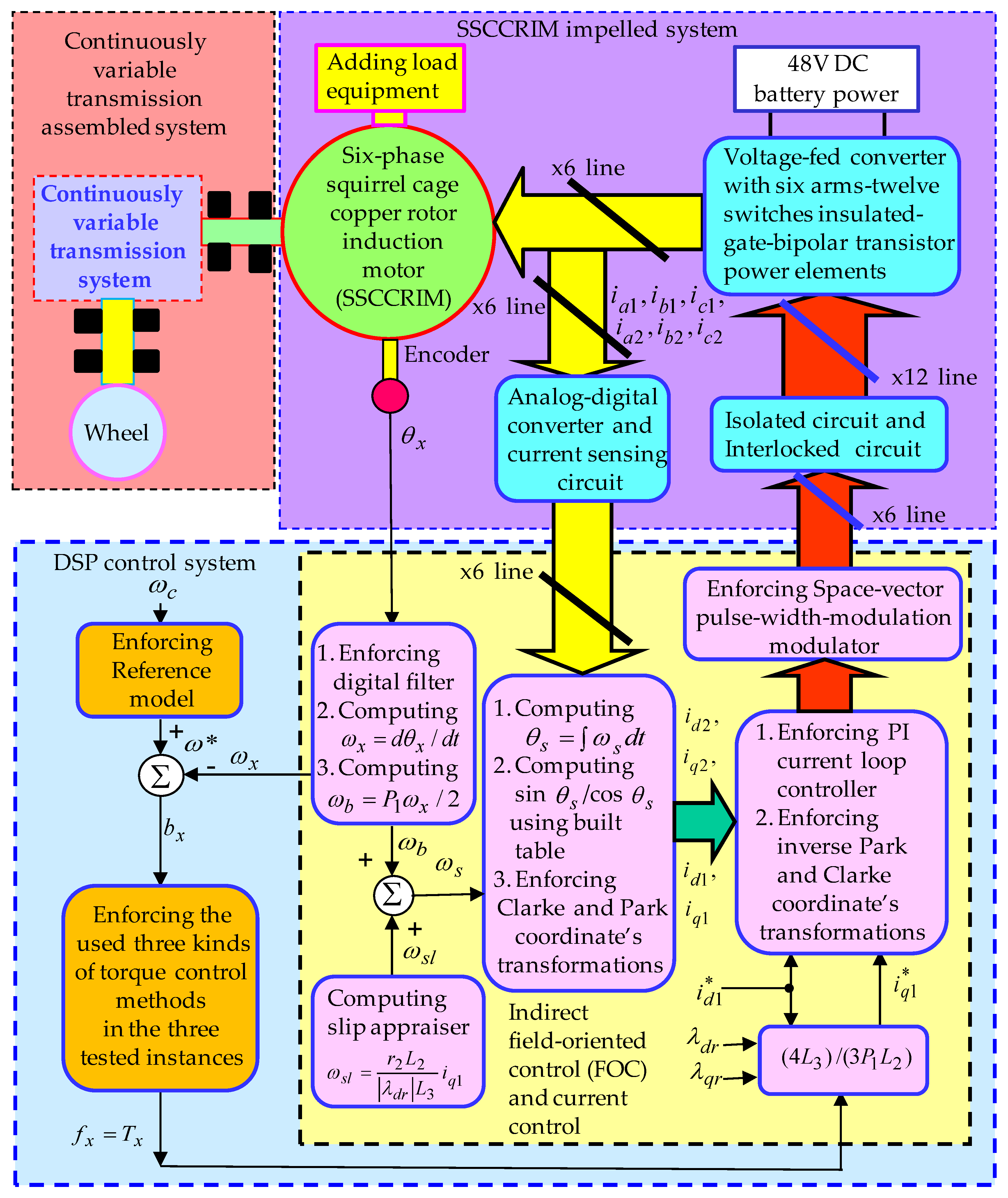
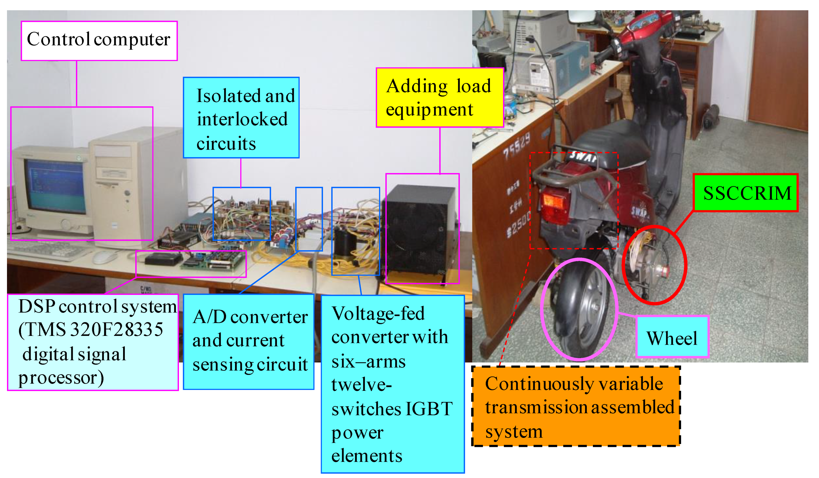
2. Descriptions of Entire System

The entire system is composed of three subsystems that are the continuously variable transmission assembled system, the SSCCRIM modeling system and the SSCCRIM impelled system. Three subsystems are described as below.

2.1. Continuously Variable Transmission Assembled System

Owing to the effects of nonlinear uncertainties, the SSCCRIM impelled continuously variable transmission assembled system conduced seriously abnormal performance variation in the entire system. The tracking responses of torque and speed control in the SSCCRIM impelled continuously variable transmission assembled system especially deteriorated under nonlinear uncertainties. Therefore, the better models in the SSCCRIM impelled continuously variable transmission assembled system are important in system modelling and control performance. The conformation of the SSCCRIM impelled continuously variable transmission assembled system is shown in Figure 1 [22,26]. Considering that the belt curve effects loss, power loss and sliding loss, which are insignificant in Figure 1, the four drive equations with simplified kinematics of the continuously variable transmission assembled system in the subordinate driven flank and the foremost driving flank by using the law of safekeeping are described as
T x = J t d ω x d t + B t ω x + T w
T w = μ y ( υ x , υ y ) ω y T z / ω x
T z = J z d ω y d t + B z ω y + T y
T y = J y d ω y d t + B y ω y + T y l ( v x y , T x y , F y l , B y , ω y 2 )
where T x , T w , T z and T y are the electromagnetic torque in the SSCCRIM, the input driving torque in the foremost pulley flank, the output driven torque in the subordinate pulley flank and the impelled torque in the wheel, respectively; J t = J x + J w and B t = B x + B w are the synthesized moment of inertia and the synthesized viscous friction coefficient, respectively; J x , J w , J z and J y are the moment of inertia in the SSCCRIM, the moment of inertia in the foremost pulley flank, the moment of inertia in the subordinate pulley flank and the moment of inertia in the wheel, respectively; B x , B w , B z and B y are the viscous frictional coefficient in the SSCCRIM, the viscous frictional coefficient in the foremost pulley flank, the viscous frictional coefficient in the subordinate pulley flank and the viscous frictional coefficient in the wheel, respectively; μ y ( υ x , υ y ) , ( υ x , υ y ) , ( ρ x , ρ y ) , ( T y , T y l ) are the transposition ratios in connection with the foremost flank and subordinate pulley flank in the continuously variable transmission assembled system, the slip arcs in connection with driving torque transmission under low speed, the wrap angles that are the contacted arcs between belt and pulley, the input transmitting torque and the output load torque on the foremost driving pulley and the subordinate driven pulley, respectively; T y l ( v x y , T x y , F y l , B y , ω y 2 ) is the intact nonlinear extrinsic disturbances in the subordinate driven pulley; v x y , T x y , F y l , ω x and ω y are the rolling resistance, the wind resistance, the braking force, the speed in the foremost pulley flank and the speed in the subordinate pulley flank, respectively. Then, the torque equation can be transformed from the subordinate pulley flank to the foremost pulley flank by use of speed ratio and sliding ratio. For simplification, the modeling of the continuously variable transmission assembled system can be assumed negligible with regard to power and slip losses. Thus, the synthesized dynamic equation in the SSCCRIM impelled continuously variable transmission assembled system from Equation (1) to Equation (4), including the synthesized torque, can be described as
J t d ω x d t + B t ω x + T y l ( Δ T w , T l y ( v x y , T x y , F y l , B y , ω y 2 ) ) + T f = T x
where T y l ( Δ T w , T l y ( v x y , T x y , F y l , B y , ω y 2 ) ) = Δ T w + T a 1 is the large nonlinear extrinsic disturbances and parameter variations; T f = T f ( T l s , T s s , T c s , T r s ) is the synthesized torque; T l s , T s s , T c s and T r s are the external load torque, the Stribeck effect torque, the cogging torque and the coulomb friction torque, respectively; Δ T w = Δ J t d ω x d t + Δ B t ω x and T a 1 = T l y ( v x y , T x y , F y l , B y , ω y 2 ) are the entire parameter variations and the entire nonlinear extrinsic disturbances, respectively.

2.2. SSCCRIM Modeling System

For simplicity in the six-phase a 1 b 1 c 1 a 2 b 2 c 2 axes coordinate frames via the Clarke and Park transformations, the voltage equations in the coordinate frames transformation from the six-phase a 1 b 1 c 1 a 2 b 2 c 2 axes to the q 1 d 1 q 2 d 2 axes in the SSCCRIM can be represented by [17,18,19]
v d 1 = r 1 i d 1 ω s λ q 1 + d λ d 1 d t
v q 1 = r 1 i q 1 + ω s λ d 1 + d λ q 1 d t
v d 2 = r 1 i d 2 + d λ d 2 d t
v q 2 = r 1 i q 2 + d λ q 2 d t
0 = r 2 i d r + ω s l λ q r + d λ d r d t
0 = r 2 i q r + ω s l λ d r + d λ q r d t
where λ q 1 = L 1 i q 1 + L 2 i q r , λ d 1 = L 1 i d 1 + L 2 i d r and λ q 2 = L 1 i q 2 , λ d 2 = L 1 i d 2 are the q 1 d 1 axes and q 2 d 2 axes flux linkages, respectively. λ q r = L 3 i q r + L 2 i q 1 , λ d r = L 3 i d r + L 2 i d 1 are the q r d r axes flux linkages. v q 1 , v d 1 , v q 2 , v d 2 are the q 1 d 1 q 2 d 2 axes voltages. i q 1 , i d 1 , i q 2 , i d 2 are the d 1 q 1 d 2 q 2 axes currents. i q r , i d r are the q r d r axes currents. r 1 and r 2 are the stator resistance and rotor resistance, respectively; L 1 , L 2 and L 3 are the stator-coil self-inductance, the mutual inductance between stator coils and rotor coils and the rotor-coil self-inductance, respectively. ω s and ω s l = ω s ω b = r 2 L 2 i q 1 / ( | λ d r | L 3 ) are the electrical angular speed of synchronous flux and the slip angular speed, respectively. ω b is the electrical angular speed of rotor. P 1 is the number of poles. The electromagnetic torque T x in the SSCCRIM can be described as
T x = k x [ λ d r i q 1 λ q r i d 1 ]
where k x = 3 P 1 L 2 / ( 4 L 3 ) is the torque constant. Besides, the dynamic equation for speed-torque of the SSCCRIM can be described as
T x = T f ( T l s , T s s , T c s , T r s ) + J x d ω x d t + B x ω x
where ω x = 2 ω b / P 1 is the mechanical angular speed of rotor in the SSCCRIM.

2.3. SSCCRIM Impelled System

The composition of the SSCCRIM impelled continuously variable transmission assembled system shown in Figure 2 is composed of three subsystems as the SSCCRIM impelled system, the continuously variable transmission assembled system and the digital signal processor (DSP) control system. The continuously variable transmission assembled system is composed of the continuously variable transmission system and the wheel. The SSCCRIM impelled system is comprised of the voltage-fed converter with six arms–twelve switches insulated-gate bipolar transistor power elements, the isolated circuit, the interlocked circuit, the analog–digital converter and the current sensing circuit. The DSP control system can realize a speed control, an indirect field-oriented control (FOC) and a proportional-integral (PI) current control. The indirect FOC is composed of a sin θ s / cos θ s production, a built table production, a coordinate transformation, an inverse coordinate transformation and a space vector pulse-width modulation control. k 1 p = 18.6 and k 1 i = k 1 p / T 1 i = 7.6 are two gains of the PI current control via certain heuristic comprehension [26,27,28] so as to obtain a significant dynamic response. The SSCCRIM impelled system was controlled by the DSP control system under entire nonlinear extrinsic disturbances and entire parameter variations.

3. Explanations of Applied Methods

The applied methods that are composed of the SRREZPNN control method and the MFSS method are as below.

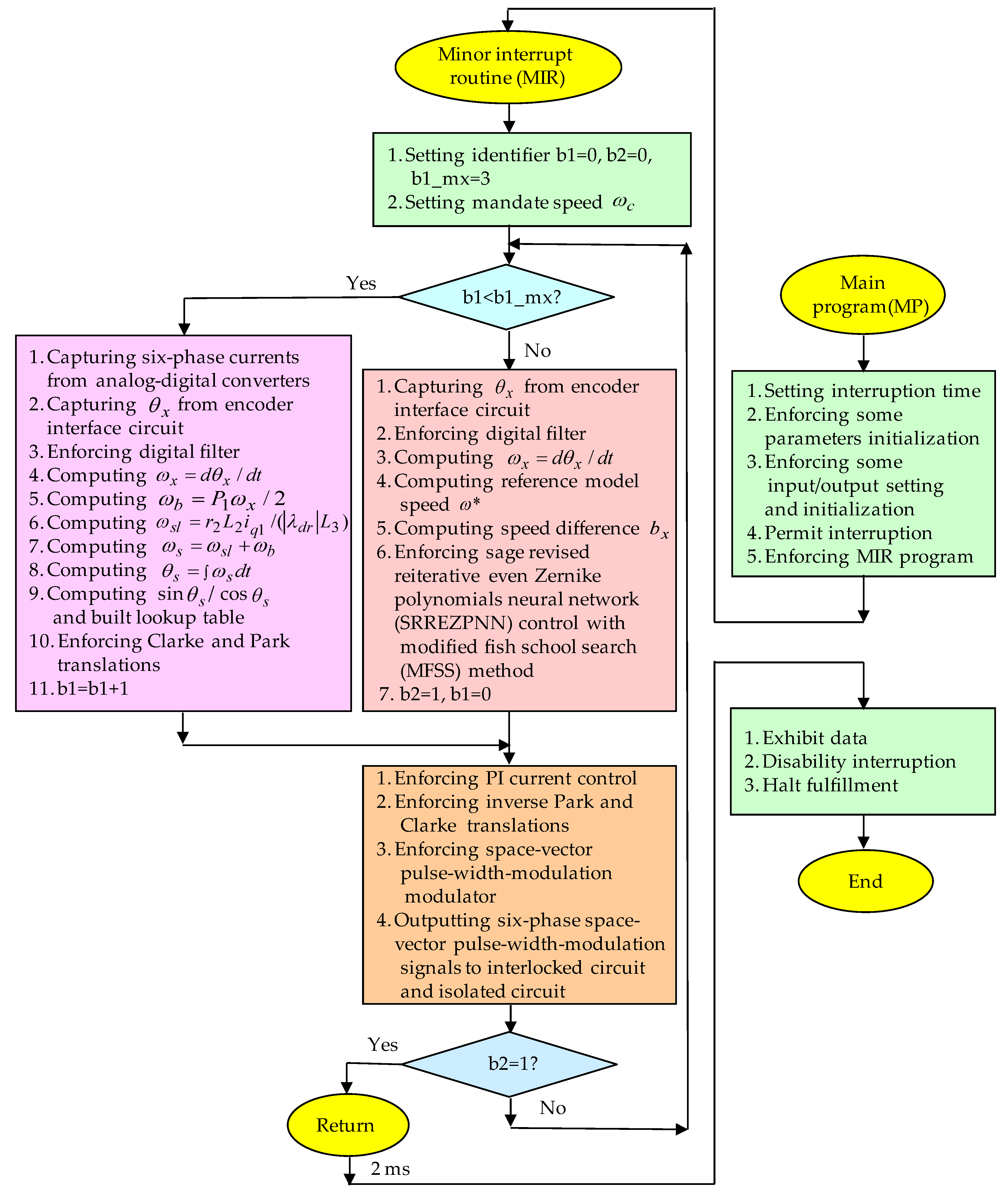
3.1. SRREZPNN Control Method

The dynamic equation in Equation (5) via systems simplification can be described as
d ω x d t = G x ω x + G y T t + G z f x
where T t = T y l ( Δ T w , T l y ( v x y , T x y , F y l , B y , ω y 2 ) ) + T f ( T l s , T s s , T c s , T r s ) = Δ T w + T a 1 + T f is the entire system’s disturbances; G x = B t / J t is an intimate ratio constant that | G x ω x | Q x ( ω x ) is assumed to be bounded and Q x ( ω x ) is the functional-bounded value; G y = 1 / J t is an intimate constant with regard to the synthesized moment of inertia that | G y T t | Q y is assumed to be bounded; G z = 1 / J t is an intimate constant the synthesized moment of inertia that G z Q z is assumed to be bounded and Q y and Q z are two bounded intimate values. f x = T x is the control torque, i.e., the electromagnetic torque of the SSCCRIM. The speed difference is defined by
b x = ω * ω x
where b x is the speed difference.
If the entire nonlinear extrinsic disturbances and the entire parameter variations are well intimate, the unflawed control rule can be described as
f x * = d ω * G z d t + k x b x G z G x ω x G z G y T t G z
where k x is a control gain that is a positive constant. When f x * = f x in Equation (16), and it is substituted into Equation (14). Then Equation (17) can be obtained as
( d d t + k x ) b x = 0
In general, when t as well as b x ( t ) 0 in Equation (17), the system’s state will track the desired trajectory. Nevertheless, the control performance of system’s state will result in sluggish tracking under the occurrence of uncertainty. Thereby, the SRREZPNN control with the MFSS method is developed for controlling the SSCCRIM impelled continuously variable transmission assembled system so as to improve speed tracking response. The control frame of the proposed control system that is depicted in Figure 3 is described as
f x = f 1 + f 2 + f 3
We can first obtain differential Equation (15), then we can substitute Equations (14) and (16) into the differential equation of (15). A difference dynamic equation can be described as
d b x d t = f x * G z f 1 G z f 2 G z f 3 G z k x b x
where f 1 is the handler control that can set the changed index I x as one to stabilize the system’s states on prescribed bound range; f 2 is the RREZPNN control that serves as the chief tracking controller so as to impersonate the unflawed control law; f 3 is the indemnified control that serves as the compensation controller so as to compensate the difference between the unflawed control and the RREZPNN control. Then, the handler control f 1 can be represented by
f 1 = I x [ 1 G z | d ω x d t | + | k x b x | G z + Q x ( ω x ) G z + Q y G z ] sgn ( b x G z )
where sgn ( ) is a sign function. When the RREZPNN approximation properties cannot be guaranteed, the handler control with the changed index I x = 1 will result in appropriate action.
The RREZPNN control f 2 shown in Figure 4 is the three-layer RREZPNN structure that is composed of a foremost layer, a middle layer and a last layer. The message disseminations in each node of each layer are described below.
Firstly, the input message and the output message in the foremost layer can be described as
v x a 1 = c g a 1 ( M )   ϕ a c 1 ( M ) l c 3 ( M 1 ) l a 1 ( M 1 ) , l a 1 ( M ) = q a 1 ( v x a 1 ) = v x a 1 , a = 1 ,   2
where Π is the multiplication factor; g 1 1 = ω * ω x = b x and g 2 1 = b x ( 1 z 1 ) = Δ b x are the speed difference and speed difference alteration, respectively; M is the iteration number; ϕ a c 1 ( M ) is the reiterative weight between the last layer and the foremost layer; q a 1 is the linear activation function; l c 3 ( M ) is the output message of node in the last layer.
Secondly, the input message and the output message in the middle layer can be described as
v x b 2 = a = 1 2 l a 1 ( M ) + ε   l b 2 ( M 1 ) ,   l b 2 ( M ) = q b 2 ( v x b 2 ) = E Z b ( v x b 2 ; s ) , b = 0 , 1 , ,   n 1
where Σ is the summation factor; ε is the reiterative gain in the middle layer; n is the number of node in the middle layer. Even Zernike polynomials function [9,29] is adopted as the activation function. E Z j ( x ; s ) is the even Zernike polynomials function with 1 < x < 1 . E Z 0 ( x ; s ) = 1 , E Z 1 ( x ; s ) = 1 + x and E Z 2 ( x ; s ) = ( 1 + x ) ( 1 + x ) + x ( s 1 ) are the zero-, one- and two-order even Zernike polynomials functions, respectively. The even Zernike polynomials function in the recurrence relation [9,29] is given by E Z m + 1 ( x ; s ) = ( 1 + x ) E Z m ( x ; s ) + x ( s m 1 ) E Z m 1 ( x ; s ) .
Thirdly, the input message and the output message in the last layer can be described as
v x k 3 = b = 0 n 1 ϕ c b 2 ( M ) l b 2 ( M ) ,   l c 3 ( M ) = q c 3 ( v x c 3 ) = v x c 3 ,   c = 1
where ϕ c b 2 ( M ) is the linking weight between the middle layer and the last layer; q c 3 is the linear activation function. The output message in the last layer can be represented by l c 3 ( M ) = f 2 . Thus, the RREZPNN control can be described as
f 2 = l c 3 ( M ) = A T Β
where A = [ ϕ 10 2 ϕ 1 , n 1 2 ] T and Β = [ l 0 2 l n 1 2 ] T are the weight vector in the last layer and the input vector in the last layer, respectively.
In addition, a minimum difference ζ so as to realize the indemnified control can be described as
ζ = ( f x * f 2 ) ( f 2 * f 2 )
where f 2 * = ( A * ) T Β is the unflawed control law of the RREZPNN control; A * is the unflawed weight vector; | ζ | < β < κ , κ < ( [ Q x ( ω x ) + Q y + | d ω x / d t | + | k x b x | ] / G z ) and κ is a small real number that is greater than zero. By using Equation (25), f 2 = l c 3 ( M ) = A T Β and f 2 * = ( A * ) T Β , then Equation (19) can be described as
d b x d t = G z f x * G z f 2 G z f 3 G z f 1 k x b x   = G z ( f x * f 2 * ) + G z ( f 2 * f 2 ) G z f 3 G z f 1 k x b x   = G z ( f x * f 2 * ) + G z [ ( A * ) T Β A T Β ] G z f 3 G z f 1 k x b x   = G z ζ + G z ( A * A ) T Β   G z f 3 G z f 1 k x b x
In order to obtain the indemnified control, the assessed law and the cozy learning law, the Lyapunov function is described as
F 1 = 0.5 b x 2 + 0.5 β ˜ 2 η 1 + 0.5 κ ˜ 2 η 2 + 0.5 ( A * A ) T ) ( A * A ) σ 1
where η 1 and η 2 are the cozy value that are greater than zero. β ˜ = β β ^ and κ ˜ = κ κ ^ are the assessed differences. σ 1 is the learning rate of the linking weight. By using Equations (25) and (26), then differential equation of the Lyapunov function can be described as
d F 1 d t = b x d b x d t β ˜ η 1 d β ^ d t κ ˜ η 2 d κ ^ d t ( A * A ) T σ 1 d   A d t   = b x { G z [ ζ + ( A * A ) T B f 3 f 1 ] k x b x } β ˜ η 1 d β ^ d t κ ˜ η 2 d κ ^ d t ( A * A ) T σ 1 d   A d t
For realizing d F 1 / d t 0 , then the indemnified control f 3 , the assessed law d υ ^ / d t and the cozy learning law d A / d t can be described as
d A d t = σ 1 Β b x G z
f 3 = ( β ^ + κ ^ ) sgn ( b x G z )
d υ ^ d t = d β ^ d t + d κ ^ d t = η 1 | b x G z | + η 2 | b x G z |
By using Equations (29)–(31) and (20) with I x = 1 , then Equation (28) can be described as
d F 1 d t = b x d b x d t β ˜ η 1 d β ^ d t κ ˜ η 2 d κ ^ d t ( A * A ) T σ 1 d   A d t = k x b x 2 + { ζ + ( A * A ) T Β ( β ^ + κ ^ ) sgn ( b x G z ) sgn ( b x G z ) [ ( Q x ( ω x ) + Q y + | d ω x / d t | + | k x b x | ) G z ] } b x G z ( β β ^ ) η 1 η 1 | b x G z | ( κ κ ^ ) η 2 η 2 | b x G z | ( ( A * A ) T σ 1 σ 1 Β G z b x = k x b x 2 +   [ ζ   b x G z β | b x G z | ] + [ κ | b x G z | sgn ( b x G z ) ( Q x ( ω x ) + Q y + | d ω x / d t | + | k x b x | ) G z b x G z ]
By using | ζ | < β < κ and κ < ( [ Q x ( ω x ) + Q y + | d ω x / d t | + | k x b x | ] / G z ) , then Equation (32) can be described as
d F 1 d t = k x b x 2 + ( ζ   b x G z β | b x G z | ) + [ κ | b x G z | sgn ( b x G z ) ( Q x ( ω x ) + Q y + | d ω x / d t | + | k x b x | ) G z G z b x ] k x b x 2 +   ( ζ β ) | b x G z | + [ κ ( Q x ( ω x ) + Q y + | d ω x / d t | + | k x b x | ) G z ] | b x G z | k x b x 2 0
when d F 1 / d t 0 in Equation (33) that is a negative semi-definite, and then b x and ( A * A ) are represented as bounded. Additionally, for the sake of proof of the proposed SRREZPNN control with the MFSS method to be gradually stable, μ ( t ) that is the uniformly continuous function can be defined by
μ ( t ) = d F 1 d t = k x b x 2
Then the integral equation of μ ( t ) can be described as
0 t μ ( τ ) d τ = 0 t   [ d F 1 d t ] d t = F 1 ( 0 ) F 1 ( t )
The differential equation of μ ( t ) can be described as
d μ d t = 2 k x b x d b x d t
The limitation of Equation (35) under F 1 ( 0 ) and F 1 ( t ) being bounded can be described as
lim t 0 t μ ( τ ) d τ <
As all variables in the right side of Equation (26) are bounded, it is implied that d b x d t is also bounded. By using Barbalat’s lemma [30,31], it can be shown that lim t 0 t μ ( τ ) d τ = 0 , thus b x ( t ) 0 as t under μ ( t ) can be a uniformly continuous function. Therefore, the SRREZPNN control with the MFSS method is gradually stable from proof. Moreover, the tracking error b x ( t ) of the system will converge to zero.
Additionally, in order to reduce chattering in the indemnified control, the sign function sgn ( b x G z ) was replaced by the continuous function b x G z / ( | b x G z | + δ ) . Then δ equals to δ 0 under | b x G z | < δ , and δ equals to zero under | b x G z | δ , where δ 0 and δ are two small real numbers that are greater than zero.
In order to train some parameters in the RREZPNN effectively, an on-line parameters training skill can be derived by using the cozy learning law d A / d t in Equation (29). Then the cozy learning law d A / d t of the parameters in the RREZPNN, the linking weight parameter by the gradient descent skill and the backpropagation skill can be denoted as
d ϕ c b 2 d t = σ 1   b   x G z g b 3  
So as to describe the online training process of the RREZPNN, an objective function can be defined by
F 2 = 0.5 b x 2
By using the gradient descent technique with the chain rule and the backpropagation technique, the cozy learning law of the linking weight ϕ c b 2 from Equation (39) can be expressed by
d ϕ c b 2 d t = σ 1 F 2 ϕ c b 2 = σ 1 F 2 b x b x l c 3 l c 3 v x c 3 v x c 3 ϕ c b 2 = σ 1 F 2 l c 3 l c 3 v x c 3 v x c 3 ϕ c b 2 = σ 1 g b 3 F 2 l c 3
In comparison with Equations (38) and (40), it can be obtained as F 2 l c 3 =   b   x G z . The updated law of the linking weight in the RREZPNN can be expressed by
ϕ c b 2 ( M + 1 ) = ϕ c b 2 ( M ) + d ϕ c b 2 d t
By using the gradient descent technique with the chain rule and the backpropagation technique, the reiterative weight ϕ a c 1 from the cozy learning law can be expressed by
d ϕ a c 1 d t = σ 2 F 2   l c 3     l c 3   l b 2     l b 2   v x b 2     v x b 2   l a 1   l a 1   v x a 1     v x a 1   ϕ a c 1 = σ 2   G z   b x ϕ c b 2 E Z j ( ) g a 1 ( M ) l c 3 ( M 1 ) l a 1 ( M )
where σ 2 is the learning rate of the reiterative weight. The updated law of the reiterative weight in the RREZPNN can be expressed by
ϕ a c 1 ( M + 1 ) = ϕ a c 1 ( M ) + d ϕ a c 1 d t
So as to obtain better convergence, the MFSS method is used for looking for two adjusted learning rates of the two weights in the RREZPNN. The proposed MFSS method not only improved convergent speed but also searched for two optimal learning rates in this study.

3.2. MFSS Method

In the MFSS method, every fish in the school realizes a local search that looks for promising regions in the search space. An individual component of the movement algorithm with regard to the learning rate can be expressed by
x n 1 , i ( t 1 + 1 ) = x n 1 , i ( t 1 ) + r a n d ( 1 , 1 ) × S p n 1 , i ,   n 1 = 1 ,   2 ,   i = 1 ,   ,   M 1 ,   t 1 = 1 ,   2 ,   ,   N 1
where x n 1 , i ( t 1 + 1 ) and x n 1 , i ( t 1 ) represent the position of the fish i before and after the individual movement operator, respectively. r a n d ( 1 , 1 ) is a uniformly distributed random number varying between −1 and 1. S p n 1 , i is the parameter that defines the maximum displacement for this movement. The new position x n 1 , i ( t 1 + 1 ) is only accepted if the fitness of the fish i improves with the position change. If it is not the case, the fish i remains in the same position, then x n 1 , i ( t 1 + 1 ) = x n 1 , i ( t 1 ) .
An average of the individual movements in the collective-instinctive component of the movement can be also expressed by
W n 1 , a v ( t 1 ) = i = 1 i = M 1 Δ x n 1 , i ( t 1 ) Δ h n 1 , i i = 1 i = M 1 Δ h n 1 , i ,   n 1 = 1 ,   2 ,   i = 1 ,   ,   M 1 ,   t 1 = 1 ,   2 ,   ,   N 1
where the vector W n 1 , a v ( t 1 ) represents the weighted average of the displacements of each fish. It means that the fishes that experienced a higher improvement will attract more fishes into its position. After the vector W n 1 , a v ( t 1 ) is computed, every fish can be expressed by
x n 1 , i ( t 1 + 1 ) = x n 1 , i ( t 1 ) + W n 1 , a v ( t 1 ) ,   n 1 = 1 ,   2 ,   i = 1 ,   ,   M 1 ,   t 1 = 1 ,   2 ,   ,   N 1
This operator in the collective-volitive component of the movement is used so as to regulate the exploration/exploitation ability of the school during the search process. First of all, the barycenter B n 1 ( t 1 ) of the school that is calculated based on the position x n 1 , i ( t 1 ) and the weight W n 1 , i ( t 1 ) of each fish i can be expressed by
B n 1 ( t 1 ) = i = 1 i = M 1 x n 1 , i ( t 1 ) W n 1 , i ( t 1 ) i = 1 i = M 1 W n 1 , i ( t 1 ) ,   n 1 = 1 ,   2 ,   i = 1 , ,   M 1 ,   t 1 = 1 ,   2 ,   ,   N 1
Besides, the movement operator was also defined as a feeding operator so as to update the weights of every fish by
W n 1 , i ( t 1 + 1 ) = W n 1 , i ( t 1 ) Δ h n 1 , i m a x ( | Δ h n 1 , i | ) ,   n 1 = 1 ,   2 ,   i = 1 ,   ,   M 1 ,   t 1 = 1 ,   2 ,   ,   N 1
where W n 1 , i ( t 1 ) is the weight parameter for fish i. Δ h n 1 , i is the fitness variation between the last and the new position. m a x ( | Δ h n 1 , i | ) represents the maximum absolute value of the fitness variation among all the fishes in the school. W n 1 , i ( t 1 ) is only allowed to vary from 1 up to W n 1 , s c a l e / 2 , which is a user defined attribute. The weights of all fishes are initialized with the value W n 1 , s c a l e / 2 . Finally, if the total school weight i = 1 i = M 1 W n 1 , i ( t 1 ) has increased from the last to the current iteration, the fishes are attracted to the barycenter B n 1 ( t 1 ) by using Equation (49) as
x n 1 , i ( t 1 + 1 ) = x n 1 , i ( t 1 ) S p n 1 , v × r a n d ( 0 , 1 ) x n 1 , i ( t 1 ) B n 1 ( t 1 ) d i s t a n c e ( x n 1 , i ( t 1 ) B n 1 ( t 1 ) ) ,   n 1 = 1 ,   2 ,   i = 1 ,   ,   M 1
If the total school weight has not improved, the fishes are spread away from the barycenter B n 1 ( t 1 ) by using Equation (50) as
x n 1 , i ( t 1 + 1 ) = x n 1 , i ( t 1 ) + S p n 1 , v × r a n d ( 0 , 1 ) x n 1 , i ( t 1 ) B n 1 ( t 1 ) d i s t a n c e ( x n 1 , i ( t 1 ) B n 1 ( t 1 ) ) ,   n 1 = 1 ,   2 ,   i = 1 ,   ,   M 1
where S p n 1 , v defines the size of the maximum displacement performed with the use of this operator. d i s t a n c e ( x n 1 , i ( t 1 ) B n 1 ( t 1 ) ) is the Euclidean distance between the fish position i and the school barycenter B n 1 ( t 1 ) . r a n d ( 0 , 1 ) is a uniformly distributed random number varying between 0 and 1. At last, x n 1 , i ( t 1 + 1 ) ,   n 1 = 1 ,   2 is the best solution in regard to the learning rates σ n 1 ( t 1 + 1 ) ,   n 1 = 1 ,   2 of the two weights in the RREZPNN. Hence, the better numbers could be optimized by using the MFSS method for adjusting two learning rates of two weights so as to find two optimal values and speed up the convergence of two weights.
Remark 1.
The control design idea for constructing the proposed SRREZPNN control with MFSS method by using the Lyapunov function is the main key point. The proposed control system is shown in Equation (18) and Figure 3, which reduces the input dimensions of the RREZPNN.
Remark 2.
RREZPNN approximation holds only in a compact set. Thus, the obtained result is semi-global in the sense that they hold for the compact sets, there exists the proposed SRREZPNN control MFSS method with a sufficiently large number of RREZPNN nodes such that all the closed-loop signals are bounded.
Remark 3.
Owing to inherent uncertainty in the SSCCRIM drive system in Equation (14), it will be shown that we cannot conclude the convergence of the tracking error to zero. Therefore, it is only reasonable to expect that all errors defined on the proposed SRREZPNN control MFSS method with the indemnified control, the assessed law and the cozy learning law converge into a neighborhood with reachable radius, and remains within it thereafter, which is so-called uniformly ultimate boundedness.

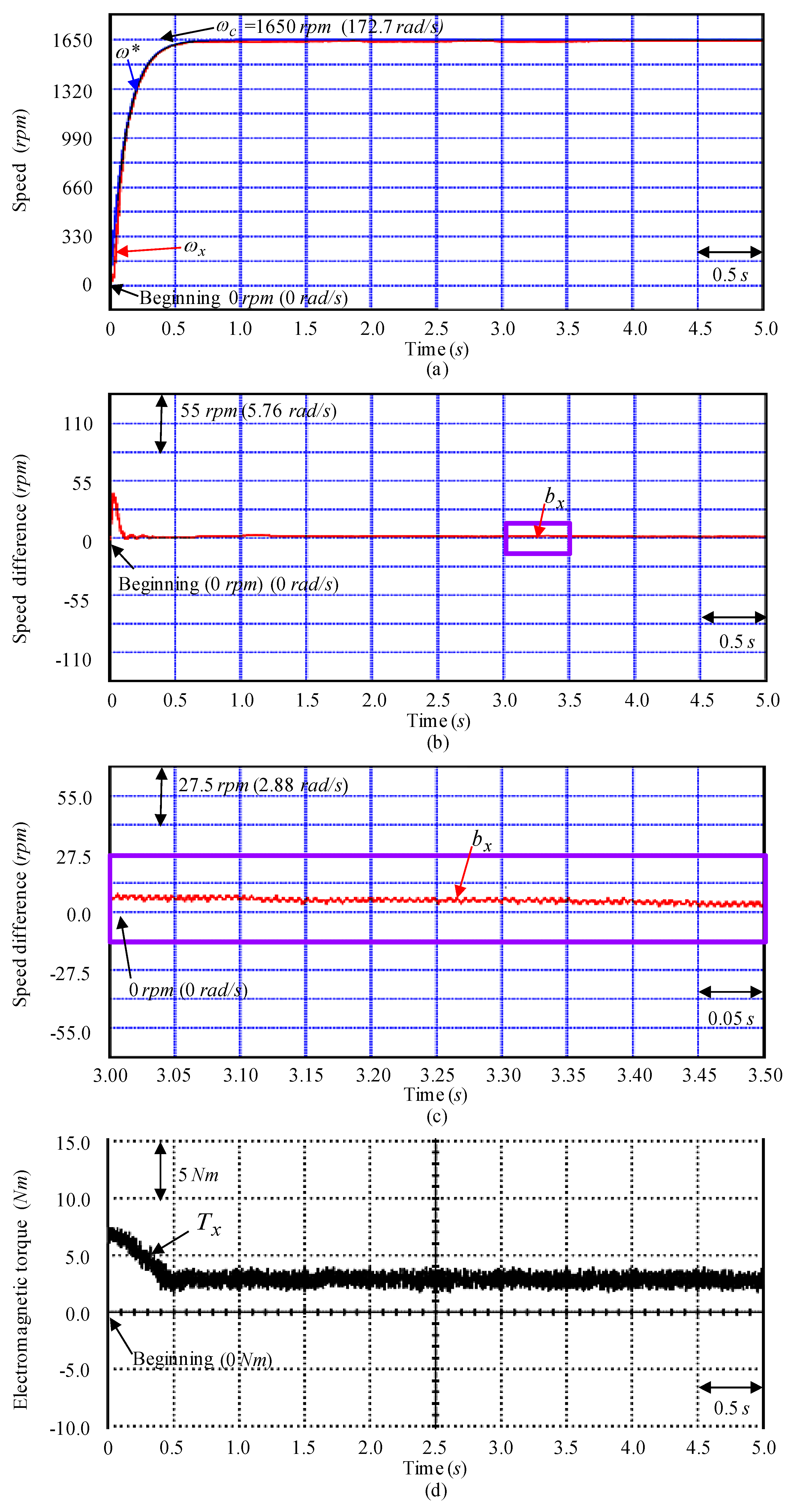
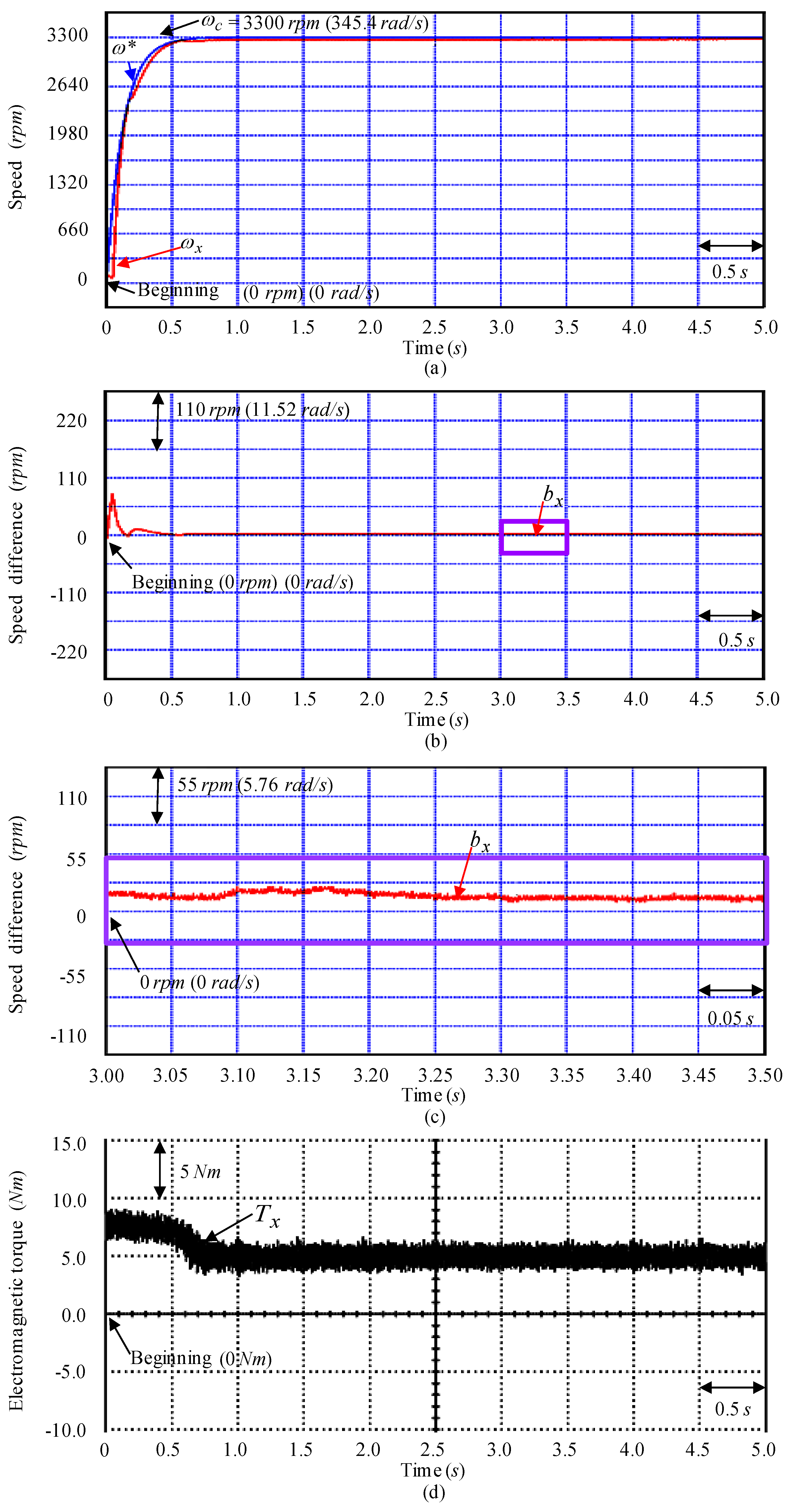
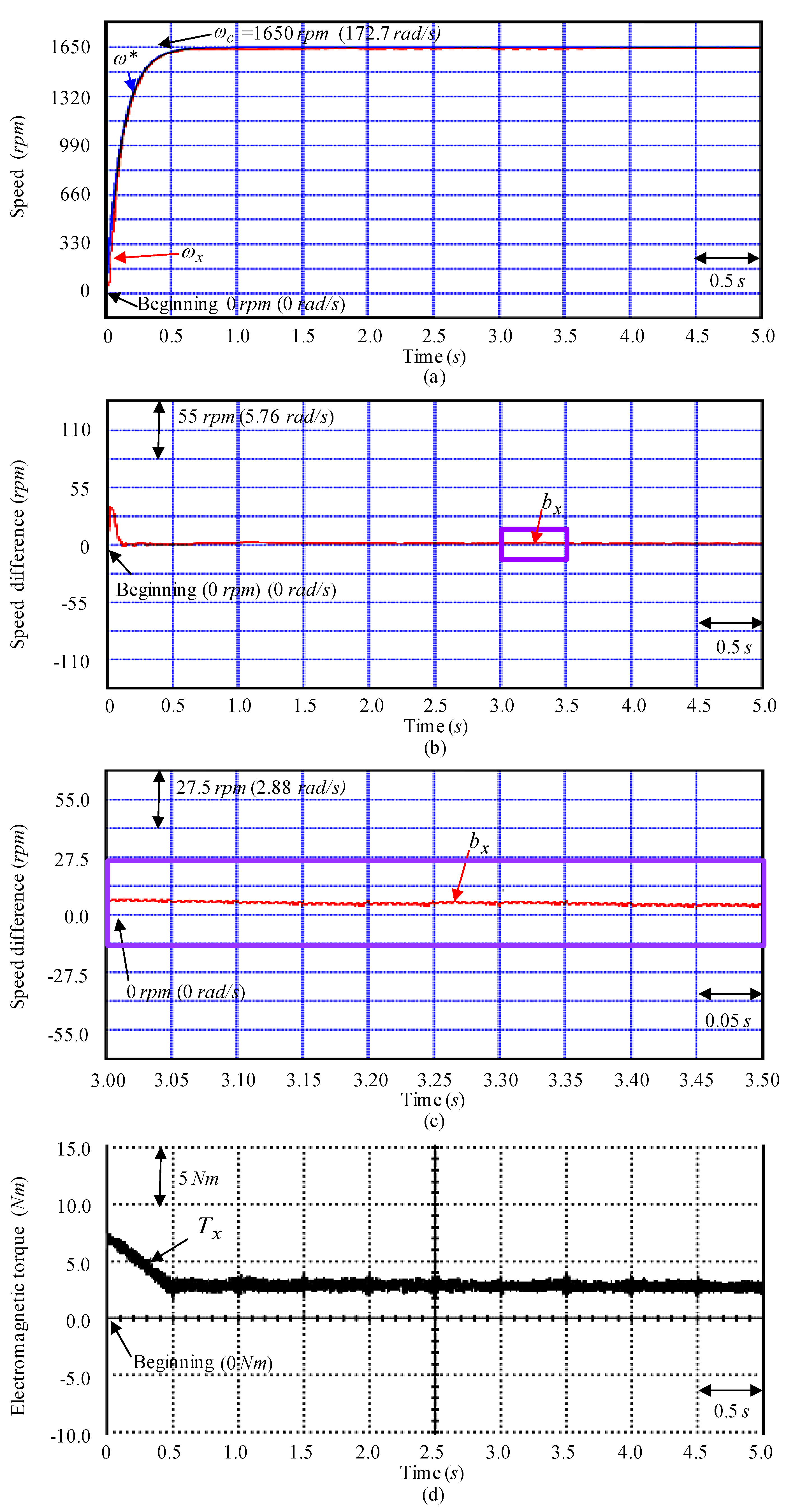
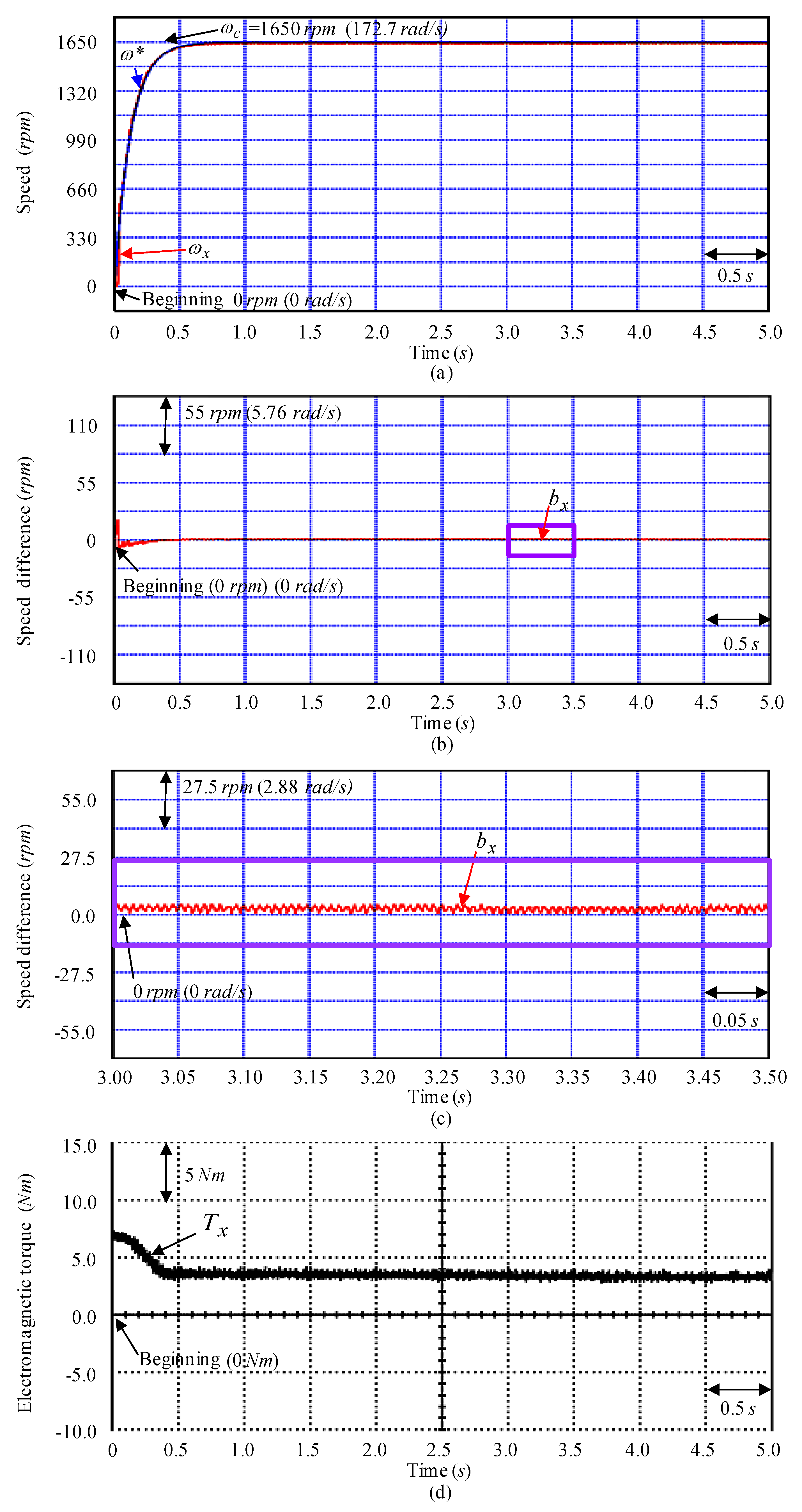
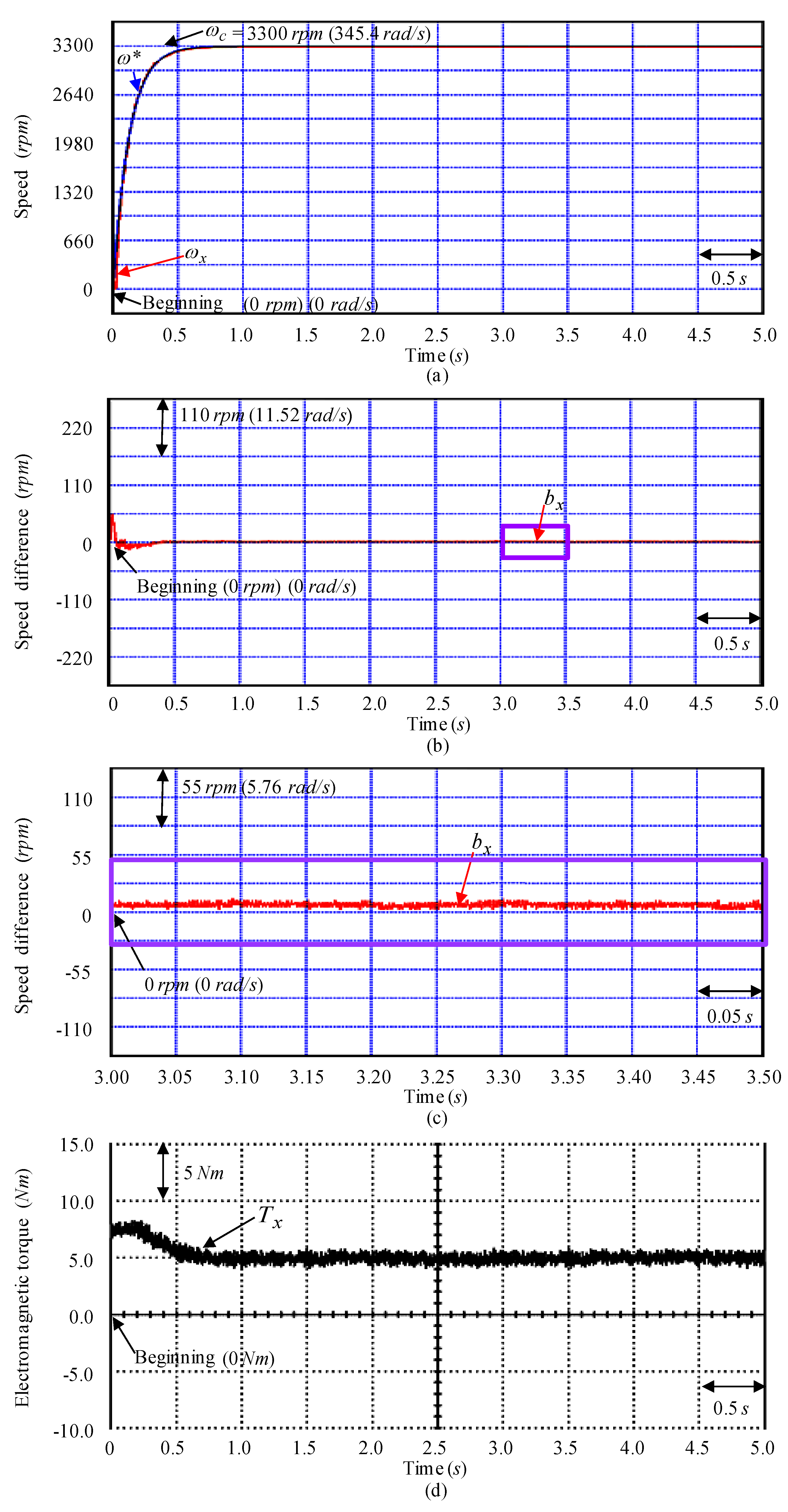
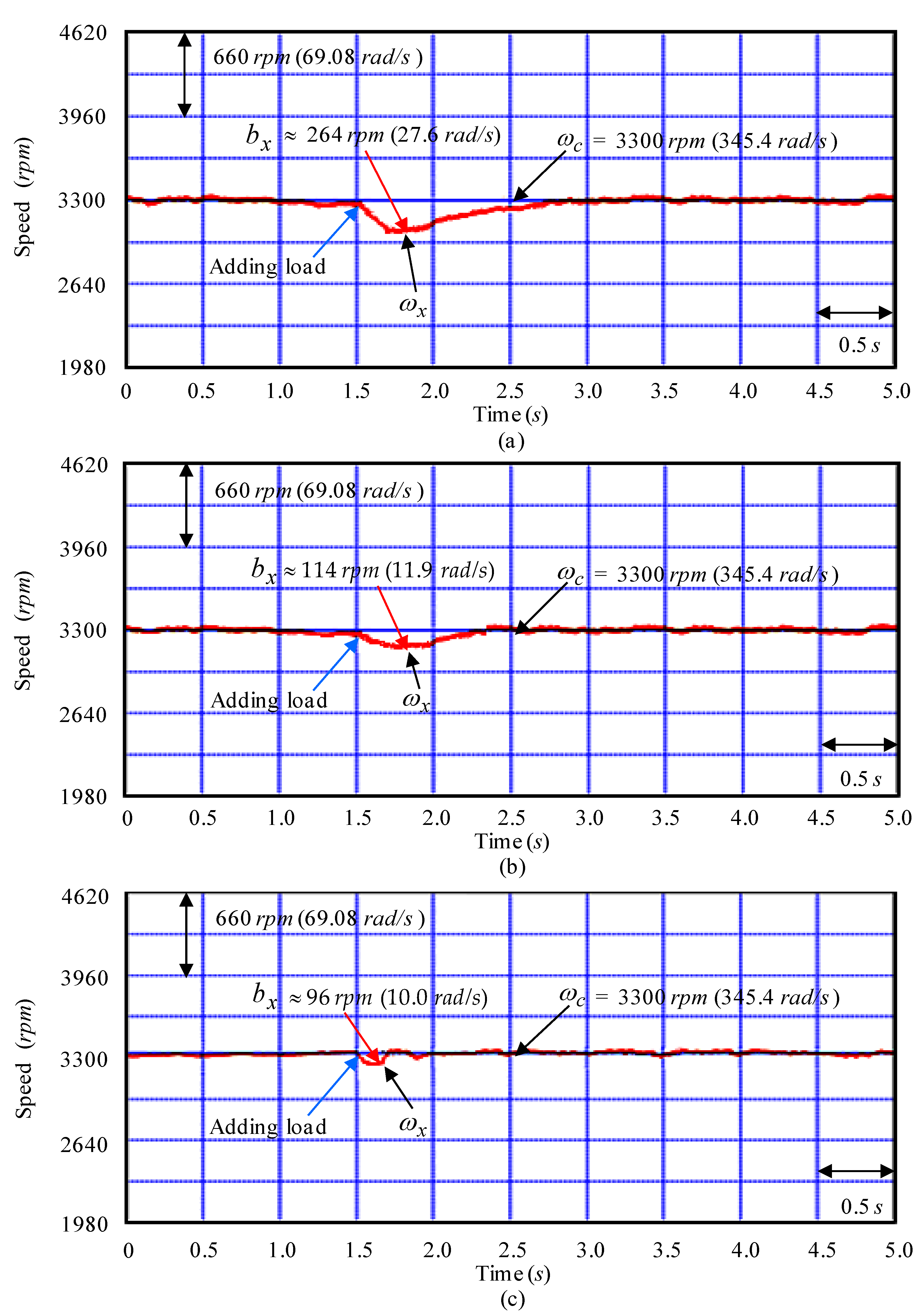
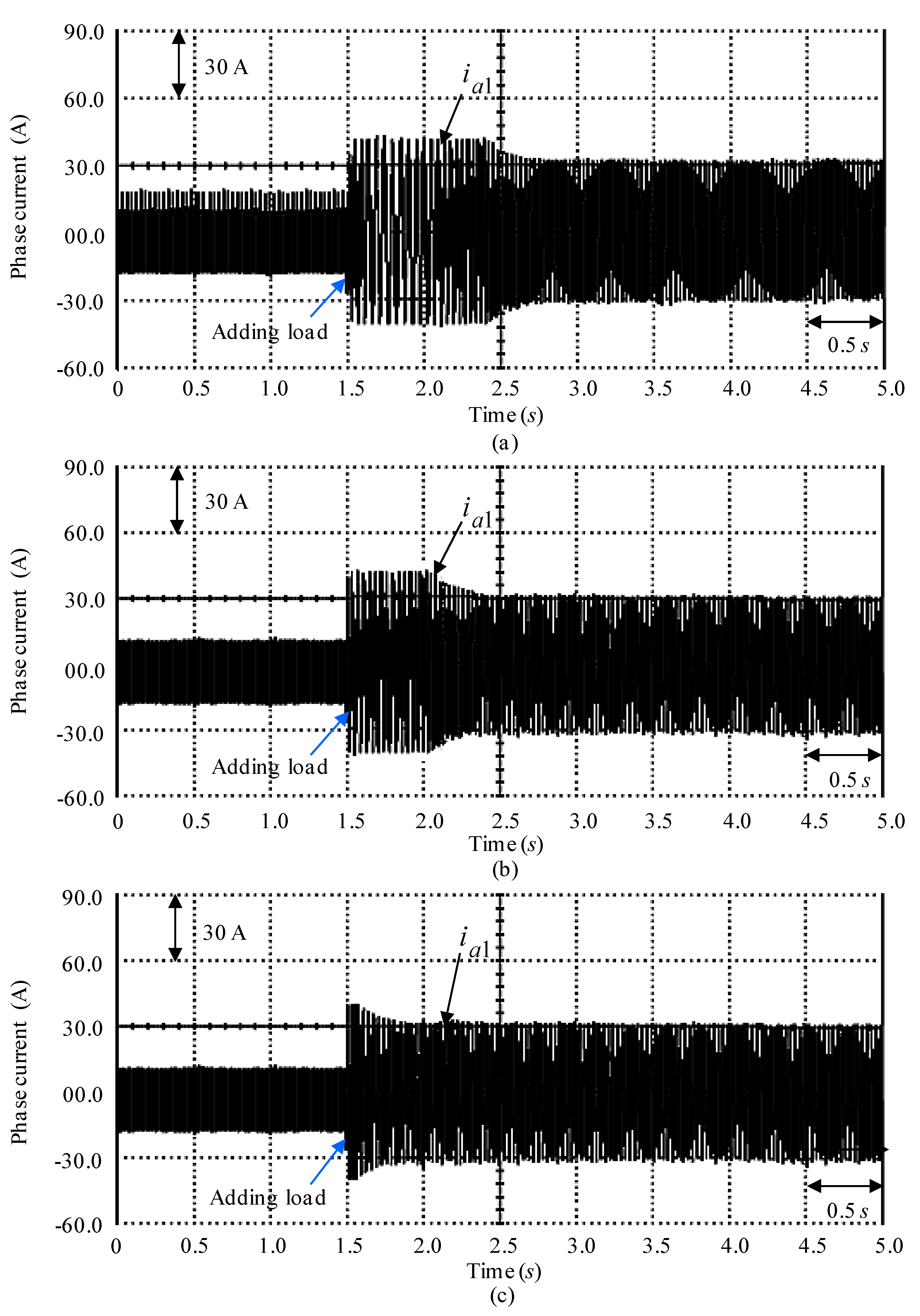
4. Tests and Experimental Results

The conformation of the SSCCRIM impelled continuously variable transmission assembled system by using DSP control system is shown in Figure 2. The profile formats of the continuously variable transmission assembled system with conversion ratio as 4.8 are the V-belt length as 652.4 mm, the subordinate pulley diameter as 75.8 mm, the foremost pulley diameter as 34.4 mm. The rated specification of the SSCCRIM is given as six-phase two-poles 48 V, 2 kW, 3452 rpm. The mechanical and electrical parameters of the SSCCRIM are as J x = 18.24 × 10 3   Nms , B x = 2.16 × 10 3   Nms / rad , k x = 0.214   Nm / A , r 1 = 1.58   Ω , r 2 = 1.21   Ω , L 1 = 19.28   mH , L 2 = 4.8   mH , L 3 = 19.12   mH . Due to the fixed uncertainty effect in the continuously variable transmission assembled system and the power output limitation in the 48 VDC battery power source, the SSCCRIM impelled continuously variable transmission assembled system is used in 3300 rpm (345.4 rad/s) so as to prevent the insulated-gate bipolar transistor power elements from burning down the SSCCRIM impelled system. Figure 5 is shown in the flowchart of the carried out control method by DSP control system in the experimental tests with real-time implementation that is composed of the main program (MP) and the minor interrupt routine (MIR). The MP realizes all settings and initializations for some parameters and input/output interfaces. The MIR realizes the interrupt process inner 2 ms. The MIR with 2 ms interrupt time processes the following works as capturing six-phase currents from analog-digital converters, capturing rotor position of the SSCCRIM from encoder, computing rotor speed, computing speed difference, enforcing lookup table and coordinate translations, enforcing PI current control, enforcing the proposed control system, and outputting six-phase space vector pulse-width modulation signals to switch the voltage-fed converter with six arms–twelve switches insulated-gate bipolar transistor power elements. Three identifiers b1, b2 and b1_mx are set as 0, 0, and 3, respectively. The DSP control system with the indirect FOC applied the identifier b2 to serve as the enforcing number of the proposed control scheme. If the indirect FOC is enforced in less than three times, i.e., b1<b1_mx, the indirect FOC needs to be enforced repeatedly. When the proposed control scheme is enforced one time and the indirect FOC is enforced three times, then the MIR will return the MP.
Three tested instances with experimental results are illustrated to demonstrate various control performances. Firstly, the one entire parameter variation and entire nonlinear extrinsic disturbances Δ T w + T a 1 case at 1650 rpm (172.7 rad/s) is the examination Y1 instance. Secondly, the double entire parameter variations and entire nonlinear extrinsic disturbances 2 Δ T w + T a 1 case at 3300 rpm (345.4 rad/s) is the examination Y2 instance. Thirdly, the adding external load torque disturbance and entire nonlinear extrinsic disturbances 2 N m ( T l s ) + T a 1 at 3300 rpm (345.4 rad/s) speed is the examination Y3 instance. Three adopted controllers are the prominent PI controller as the controller CD1, the Mixed modified recurring Rogers-Szego polynomials neural network (MMRRSPNN) control with mended grey wolf optimization (MGWO) [13] as the controller CD2 and the proposed SRREZPNN control with the MFSS method as the controller CD3 so as to compare with control performances. Firstly, two gains k 2 p = 21.2 and k 2 i = k 2 p / T 2 i = 5.2 in the controller CD1 can be obtained by using the Kronecker method [26,27,28] that is used to narrow down the region for iterative selection of values of the parameters of k 2 p and k 2 i on the tuning of the PI controller with one entire parameter variations and entire nonlinear extrinsic disturbances Δ T w + T a 1 case at 1650 rpm (172.7 rad/s) for the speed tracking to achieve better stability boundary in the k 2 p and k 2 i plane so as to get better transient-state and steady-state control performance. Secondly, some control gains k a = 4.52 , η = 0.08 and   γ = 0.18 in the controller CD2 can be obtained to show better transient control performance under the requirement of stability consideration. Additionally, the neuron’s numbers of the MRRSPNN are 2, 3 and 1 nodes in the first layer, the second layer and the third layer of MRRSPNN, respectively. Thirdly, some control gains by using the controller CD3 are given as k x = 4.52 ,   ε = 0.08 , η 1 = 0.18 and η 2 = 0.18 to attain better transient control performance under the requirement of stability consideration. In addition, the neuron’s numbers of the RREZPNN are 2, 3 and 1 nodes in the foremost layer, the middle layer and the last layer of the RREZPNN, respectively.
Firstly, Figure 6 and Figure 7 display some experimental results by using the controller CD1 for the SSCCRIM impelled continuously variable transmission assembled system at the examination Y1 instance and at the examination Y2 instance. The speed responses for mandate speed ω c , reference model speed ω * , and gauged speed ω x at two tested instances are shown in Figure 6a and Figure 7a. The speed difference b x responses at two tested instances are shown in Figure 6b and Figure 7b. The enlargements of speed difference responses at two tested instances are shown in Figure 6c and Figure 7c. The electromagnetic torque T x responses are shown in Figure 6d and Figure 7d. Figure 6a at the examination Y1 instance demonstrated better speed tracking performance because small disturbance is the same with the rated instance. Figure 7a demonstrated dilatory speed responses because of absent gains adjustment appropriately. Moreover, Figure 6d and Figure 7d in the electromagnetic torque T x responses demonstrated large torque ripple because of large nonlinear operation in the continuously variable transmission assembled system.
Secondly, Figure 8 and Figure 9 display some experimental results by using the controller CD2 for the SSCCRIM impelled continuously variable transmission assembled system at the examination Y1 instance and at the examination Y2 instance. The speed responses for mandate speed ω c , reference model speed ω * , and gauged speed ω x at two tested instances are shown in Figure 8a and Figure 9a. The speed difference b x responses at two tested instances are shown in Figure 8b and Figure 9b. The enlargements of speed difference responses at two tested instances are shown in Figure 8c and Figure 9c. The electromagnetic torque T x responses are shown in Figure 8d and Figure 9d. Figure 8a at the examination Y1 instance demonstrated better speed tracking performance because small disturbance is the same with the rated instance. Figure 9a demonstrated better speed responses owing to the online adjustable method of the MRRHPNN control system with MGWO and the compensated controller action. Moreover, Figure 8d and Figure 9d in the electromagnetic torque T x responses demonstrated middle torque ripple because of large nonlinear action in the continuously variable transmission assembled system.
Thirdly, Figure 10 and Figure 11 display some experimental results by using the controller CD3 for the SSCCRIM impelled continuously variable transmission assembled system at the examination Y1 instance and at the examination Y2 instance. The speed responses for mandate speed ω c , reference model speed ω * , and gauged speed ω x at two tested instances are shown in Figure 10a and Figure 11a. The speed difference b x responses at two tested instances are shown in Figure 10b and Figure 11b. The enlargements of speed difference responses at two tested instances are shown in Figure 10c and Figure 11c. The electromagnetic torque T x responses are shown in Figure 10d and Figure 11d. Figure 10a at the examination Y1 instance demonstrated better speed tracking performance because small disturbance is the same with the rated instance. Figure 11a displayed better speed responses because of the online cozy mechanism of the RREZPNN and the indemnified control’s motion. Moreover, the smaller torque ripple responses displayed in Figure 10d and Figure 11d for the electromagnetic torque T x are due to online adjustment of the SRREZPNN control with the MFSS method to overcome the unmodeled dynamic of continuously variable transmission assembled system such as V-belt torsion and push–pull frictions.
Besides, Figure 12a,b demonstrate the convergent responses for learning rate σ 1 of linking weight and learning rate σ 2 of reiterative weight in the SRREZPNN control with the MFSS method as the controller CD3 at the examination Y1 instance, respectively. Figure 12c,d demonstrate the convergent responses for learning rate σ 1 of linking weight and learning rate σ 2 of reiterative weight in the SRREZPNN control with the MFSS method as the controller CD3 at the examination Y2 instance, respectively.
At last, the speed-regulated responses and the gauged phase current a 1 responses obtained by using the controller CD1, the controller CD2 and the controller CD3 under adding external load torque disturbance and entire nonlinear extrinsic disturbances 2 N m ( T l s ) + T a 1 at 3300 rpm speed as the examination Y3 instance are shown in Figure 13 and Figure 14. The tested instances with experimental results of gauged speed ω x and gauged phase current i a 1 at the examination Y3 instance when the controller CD1, the controller CD2 and the controller CD3 are shown in Figure 13 and Figure 14. The speed-regulated responses for mandate speed ω c and gauged speed ω x in the examination Y3 instance case by using the controller CD1, the controller CD2 and the controller CD3 are displayed in Figure 13a–c, respectively. The gauged phase current a 1 responses at the examination Y3 instance case by using the controller CD1, the controller CD2 and the controller CD3 are displayed in Figure 14a–c, respectively. The tested instances with experimental results display that the degenerated responses at the examination Y3 instance are fairly improved when the controller CD3 was used. Besides, transient response of the controller CD3 displays better convergence and better load regulation than the controller CD1 and the controller CD2.
Finally, the photo of the test rig and experimental setup is shown in Figure 15.

5. Discussions and Analyses

Dynamic responses for control performances in comparison with the prominent PI controller as the controller CD1, the MMRRSPNN with MGWO [13] as the controller CD2, and the proposed SRREZPNN control with the MFSS method as the controller CD3 for three tested instances with experimental results are explained as below. The maximum differences of b x obtained by using the controllers CD1, CD2 and CD3 at the Examination Y1 instance are 73 rpm (7.64 rad/s), 58 rpm (6.07 rad/s) and 31 rpm (3.24 rad/s), respectively. The root mean square differences of b x obtained by using the controllers CD1, CD2 and CD3 at the Examination Y1 instance are 37 rpm (3.87 rad/s), 18 rpm (1.88 rad/s) and 13 rpm (1.36 rad/s), respectively. The maximum differences of b x obtained by using the controllers CD1, CD2 and CD3 at the Examination Y2 instance are 136 rpm (14.23 rad/s), 79 rpm (8.27 rad/s) and 41 rpm (4.29 rad/s), respectively. The root mean square differences of b x obtained by using the controllers CD1, CD2 and CD3 at the Examination Y2 instance are 52 rpm (5.44 rad/s), 28 rpm (2.93 rad/s) and 19 rpm (1.99 rad/s), respectively. The maximum differences of b x obtained by using the controllers CD1, CD2 and CD3 at the Examination Y3 instance are 264 rpm (27.63 rad/s), 114 rpm (11.93 rad/s) and 96 rpm (10.05 rad/s), respectively. The root mean square differences of b x obtained by using the controllers CD1, CD2 and CD3 at the Examination Y3 instance are 49 rpm (5.13 rad/s), 24 rpm (2.51 rad/s) and 16 rpm (1.67 rad/s), respectively.
Moreover, the feature performances in comparison with the controllers CD1, CD2 and CD3 on the basis of three tested instances with experimental results are recapitulated as below. The oscillation values in the control laws obtained by using the controller CD1, the controller CD2 and the controller CD3 are the 12% of rated value, the 9% of rated value and the 5% of rated value at the Examination Y2 instance, respectively. The movement responses obtained by using the controller CD1, the controller CD2 and the controller CD3 are the 2.1 s rising time, the 1.7 s rising time and the 1.5 s rising time at the Examination Y2 instance, respectively. The adjustment capabilities for external load torque disturbance obtained by using the controller CD1, the controller CD2 and the controller CD3 are the 264 rpm (27.63 rad/s) maximum difference, the 144 rpm (11.93 rad/s) maximum difference and the 96 rpm (10.05 rad/s) maximum difference at the Examination Y3 instance, respectively. The convergent speeds obtained by using the controller CD1, the controller CD2 and the controller CD3 are the 2.4 s settle time, the 2.1 s settle time and the 1.7 s settle time at the Examination Y2 instance, respectively. The speed tracking differences obtained by using the controller CD1, the controller CD2 and the controller CD3 are the maximum difference as 136 rpm (14.23 rad/s), the maximum difference as 79 rpm (8.27 rad/s) and the maximum difference as 41 rpm (4.29 rad/s) at the Examination Y2 instance, respectively. The repudiation abilities for parameter disturbance obtained by using the controller CD1, the controller CD2 and the controller CD3 are the maximum difference as 136 rpm (14.23 rad/s), the maximum difference as 79 rpm (8.27 rad/s) and the maximum difference as 41 rpm (4.29 rad/s) at the Examination Y2 instance, respectively. The two learning rates obtained by using the controller CD1, the controller CD2 and the controller CD3 are the none, the two varying values as two optimal learning rates and the two varying values as two optimal learning rates, respectively. The calculation times of NN obtained by using the controller CD1, the controller CD2 and the controller CD3 are the none, the 0.18 ms and the 0.12 ms, respectively. The torque ripples with belt trembling and torsional fluctuation obtained by using the controller CD1, the controller CD2 and the controller CD3 are the 12% of rated value, the 8% of rated value and the 8% of rated value at the Examination Y2 instance, respectively. From these performances with respect to the oscillation values in the control laws, the movement responses, the adjustment capabilities for external load torque disturbance, the convergent speeds, the speed tracking differences, the repudiation abilities of parameter disturbance, the calculation times of NN and torque ripples in the controller CD3 are better than the controllers CD1 and CD2.

6. Conclusions

The SRREZPNN control with the MFSS method has been successfully applied to control the SSCCRIM impelled continuously variable transmission assembled system with better robustness. The SRREZPNN control with MFSS method that can realize the handler control, the RREZPNN control and the indemnified control were proposed to reduce the control intensity with smoothing when the system’s states are within the predictive bounded region.
The core contributions of this study are described below. (1) The mathematic models of SSCCRIM impelled continuously variable transmission assembled system with nonlinear uncertainties have been successfully reduced by the four simplified dynamic models. (2) The SSCCRIM impelled continuously variable transmission assembled system under intact nonlinear extrinsic disturbances effect has been successfully controlled by using the SRREZPNN control with the MFSS method. (3) According to the Lyapunov stability theorem, the cozy learning law in the RREZPNN control and the assessed law in the indemnified control have been successfully derived. (4) The MFSS method was well utilized to adjust two learning rates of linking and reiterative weights in the RREZPNN to obtain optimal values and speed up convergence of linking and reiterative weights. (5) The SRREZPNN control with MFSS method as the controller CD3 is better than the prominent PI controller as the controller CD1 and the MMRRSPNN with MGWO [13] as the controller CD2 in torque ripple demotion.
Finally, the controller CD3 is more excellent than the controller CD1 and the controller CD2 from all experimental results and control performances for the SSCCRIM impelled continuously variable transmission assembled system.
The research’s directions in future works are as below. (1) The advancement of more accurate modellings in the continuously variable transmission assembled system will be derived so as to obtain more exact experimental results. (2) High performance of the DSP control systems will be adopted to reduce execution time and enhance computation efficiency. (3) The more advanced control methods combined with this study will be adopted so as to heighten robustness in the SSCCRIM impelled continuously variable transmission assembled system. (4) The advanced control structures with tracking for some different reference trajectories will be developed so as to enhance feasibility of the control systems.

Funding

This research was funded by the Ministry of Science and Technology of Taiwan (Project MOST 108-2221-E-239-011-MY2).

Acknowledgments

The author would like to acknowledge the financial support of the Ministry of Science and Technology of Taiwan under grant MOST 108-2221-E-239-011-MY2.

Conflicts of Interest

The author declares no conflict of interest.

References

  1. Shih, P.C.; Chiu, C.Y.; Chou, C.H. Using dynamic adjusting NGHS-ANN for predicting the recidivism rate of commuted prisoners. Mathematics 2019, 7, 1187. [Google Scholar] [CrossRef] [Green Version]
  2. Behzad, M.; Mahyar, G.; Mohammad, H.A.; Heydar, M.; Shahabddin, S. Moisture estimation in cabinet dryers with thin-layer relationships using a genetic algorithm and neural network. Mathematics 2019, 7, 1042. [Google Scholar]
  3. Shao, Y.E.; Lin, S.C. Using a time delay neural network approach to diagnose the out-of-control signals for a multivariate normal process with variance shifts. Mathematics 2019, 7, 959. [Google Scholar] [CrossRef] [Green Version]
  4. Heydar, M.; Milad, S.; Mohammad, H.A.; Ravinder, K.; Shahaboddin, S. Modeling and efficiency optimization of steam boilers by employing neural networks and response-surface method (RSM). Mathematics 2019, 7, 629. [Google Scholar]
  5. Chak, C.H.; Feng, G.; Cheng, C.H. Orthogonal polynomials neural network for function approximation and system modeling. In Proceedings of the IEEE International Conference on Neural Networks, Perth, Australia, 27 November–1 December 1995; p. 5255864. [Google Scholar]
  6. Purwar, S.; Kar, I.N.; Jha, A.N. On-line system identification of complex systems using Chebyshev neural networks. Appl. Soft Comput. 2007, 7, 364–372. [Google Scholar] [CrossRef]
  7. Wang, L.; Duan, M.; Duan, S. Memristive Chebyshev neural network and its applications in function approximation. Math. Probl. Eng. 2013, 2013, 429402. [Google Scholar] [CrossRef]
  8. Lin, C.H. Comparative dynamic control for continuously variable transmission with nonlinear uncertainty using blend amend recurrent Gegenbauer-functional-expansions neural network. Nonlinear Dyn. 2017, 87, 1467–1493. [Google Scholar] [CrossRef]
  9. Iskander, D.R.; Collins, M.J.; Davis, B. Optimal modeling of corneal surfaces with Zernike polynomials. IEEE Trans. Biomed. Eng. 2001, 48, 87–95. [Google Scholar] [CrossRef]
  10. Wong, W.C.; Chee, E.; Li, J.; Wang, X. Recurrent neural network-based model predictive control for continuous pharmaceutical manufacturing. Mathematics 2018, 6, 242. [Google Scholar] [CrossRef] [Green Version]
  11. Rubio, J.J.; Yu, W. Nonlinear system identification with recurrent neural networks and dead-zone Kalman filter algorithm. Neurocomputing 2007, 70, 2460–2466. [Google Scholar] [CrossRef]
  12. Abbasvandi, Z.; Nasrabadi, A.M. A self-organized recurrent neural network for estimating the effective connectivity and its application to EEG data. Comput. Biol. Med. 2019, 110, 93–107. [Google Scholar] [CrossRef]
  13. Chen, D.F.; Shih, Y.C.; Li, S.C.; Chen, C.T.; Ting, J.C. Mixed modified recurring Rogers-Szego polynomials neural network control with mended grey wolf optimization applied in SIM expelling system. Mathematics 2020, 8, 754. [Google Scholar] [CrossRef]
  14. Carmelo, J.A.B.F.; Fernando, B.L.N.; Anthony, J.C.C.L.; Antonio, I.S.N.; Marilia, P.L. A novel search algorithm based on fish school behavior. In Proceedings of the IEEE International Conference on Systems, Man, and Cybernetics, Singapore, 12–15 October 2008; pp. 2646–2651. [Google Scholar]
  15. Salomao, S.M.; Fernando, B.L.N.; Carmelo, J.A.B.F.; Elliackin, M.N.F. Density as the segregation mechanism in fish school search for multimodal optimization problems. In Proceedings of the International Conference in Swarm Intelligence (ICSI 2011): Advances in Swarm Intelligence, Chongqing, China, 12–15 June 2011; pp. 563–572. [Google Scholar]
  16. Fernando, B.L.N.; Marcelo, G.P.L. Weight based fish school search. In Proceedings of the IEEE International Conference on Systems Man, and Cybernetics (SMC), San Diego, CA, USA, 5–8 October 2014; p. 14790101. [Google Scholar]
  17. Munoz, A.R.; Lipo, T.A. Dual stator winding induction machine drive. IEEE Trans. Ind. Appl. 2000, 36, 1369–1379. [Google Scholar] [CrossRef]
  18. Ojo, O.; Davidson, I.E. PWM-VSI inverter assisted stand-alone dual stator winding induction generator. IEEE Trans. Ind. Appl. 2000, 36, 1604–1611. [Google Scholar]
  19. Singh, G.K.; Nam, K.; Lim, S.K. A simple indirect field-oriented control scheme for multiphase induction machine. IEEE Trans. Ind. Electron. 2005, 52, 1177–1184. [Google Scholar] [CrossRef]
  20. Lin, C.H.; Hwang, C.C. Multiobjective optimization design for a six-phase copper rotor induction motor mounted with a scroll compressor. IEEE Trans. Magn. 2016, 52, 9401604. [Google Scholar] [CrossRef]
  21. Lin, C.H. Altered grey wolf optimization and Taguchi method with FEA for six-phase copper squirrel cage rotor induction motor design. Energies 2020, 13, 2282. [Google Scholar] [CrossRef]
  22. Srivastava, N.; Haque, I. Transient dynamics of metal V-belt CVT: Effects of bandpack slip and friction characteristic. Mech. Mach. Theory 2008, 43, 457–479. [Google Scholar] [CrossRef]
  23. Srivastava, N.; Haque, I. A review on belt and chain continuously variable transmissions (CVT): Dynamics and control. Mech. Mach. Theory 2009, 44, 19–41. [Google Scholar] [CrossRef]
  24. Lin, C.H. Modelling and control of six-phase induction motor servo-driven continuously variable transmission system using blend modified recurrent Gegenbauer orthogonal polynomial neural network control system and amended artificial bee colony optimization. Int. J. Numer. Model. Electron. Netw. Devices Fields 2016, 29, 915–942. [Google Scholar] [CrossRef]
  25. Lin, C.H. Blend modified recurrent Gegenbauer orthogonal polynomial neural network control for six-phase copper rotor induction motor servo-driven continuously variable transmission system using amended artificial bee colony optimization. Trans. Inst. Meas. Control 2017, 39, 921–950. [Google Scholar] [CrossRef]
  26. Astrom, K.J.; Hagglund, T. PID Controller: Theory, Design, and Tuning; Instrument Society of America: Research Triangle Park, NC, USA, 1995. [Google Scholar]
  27. Hagglund, T.; Astrom, K.J. Revisiting the Ziegler-Nichols tuning rules for PI control. Asian J. Control 2002, 4, 364–380. [Google Scholar] [CrossRef]
  28. Hagglund, T.; Astrom, K.J. Revisiting the Ziegler-Nichols tuning rules for PI control-part II: The frequency response method. Asian J. Control 2004, 6, 469–482. [Google Scholar] [CrossRef]
  29. Rdzanek, W.P. Sound radiation of a vibrating elastically supported circular plate embedded into a flat screen revisited using the Zernike circle polynomials. J. Sound Vib. 2018, 434, 91–125. [Google Scholar] [CrossRef]
  30. Astrom, K.J.; Wittenmark, B. Adaptive Control; Addison-Wesley: New York, NY, USA, 1995. [Google Scholar]
  31. Slotine, J.J.E.; Li, W. Applied Nonlinear Control; Prentice-Hall: Englewood Cliffs, NJ, USA, 1991. [Google Scholar]
Figure 1. Conformation of the SSCCRIM and the continuously variable transmission assembled system.
Mathematics 08 01760 g001
Figure 2. Composition of the SSCCRIM impelled continuously variable transmission assembled system.
Mathematics 08 01760 g002
Figure 3. Block diagram of the SRREZPNN control with MFSS method.
Mathematics 08 01760 g003
Figure 4. Constitution of the RREZPNN.
Mathematics 08 01760 g004
Figure 5. Flowchart of the carried-out program by using digital signal processor (DSP) control system.
Mathematics 08 01760 g005
Figure 6. Tested instances with experimental results obtained by using the controller CD1 for the SSCCRIM impelled continuously variable transmission assembled system at the examination Y1 instance: (a) speed response, (b) speed difference response, (c) enlargement of speed difference response, (d) electromagnetic torque response.
Mathematics 08 01760 g006
Figure 7. Tested instances with experimental results obtained by using the controller CD1 for the SSCCRIM impelled continuously variable transmission assembled system at the examination Y2 instance: (a) speed response, (b) speed difference response, (c) enlargement of speed difference response, (d) electromagnetic torque response.
Mathematics 08 01760 g007
Figure 8. Tested instances with experimental results obtained by using the controller CD2 for the SSCCRIM impelled continuously variable transmission assembled system at the examination Y1 instance: (a) speed response, (b) speed difference response, (c) enlargement of speed difference response, (d) electromagnetic torque response.
Mathematics 08 01760 g008
Figure 9. Tested instances with experimental results obtained by using the controller CD2 for the SSCCRIM impelled continuously variable transmission assembled system at the examination Y2 instance: (a) speed response, (b) speed difference response, (c) enlargement of speed difference response, (d) electromagnetic torque response.
Mathematics 08 01760 g009
Figure 10. Tested instances with experimental results obtained by using the controller CD3 for the SSCCRIM impelled continuously variable transmission assembled system obtained at the examination Y1 instance: (a) speed response, (b) speed difference response, (c) enlargement of speed difference response, (d) electromagnetic torque response.
Mathematics 08 01760 g010
Figure 11. Tested instances with experimental results obtained by using the controller CD3 for the SSCCRIM impelled continuously variable transmission assembled system at the examination Y2 instance: (a) speed response, (b) speed response, (c) enlargement of speed difference response, (d) electromagnetic torque response.
Mathematics 08 01760 g011
Figure 12. Tested instances with experimental results obtained by using the controller CD3: (a) convergent response of learning rate σ 1 of linking weight at the examination Y1 instance, (b) convergent response of learning rate σ 2 of reiterative weight at the examination Y1 instance, (c) convergent response of learning rate σ 1 of linking weight at the examination Y2 instance, (d) convergent response of learning rate σ 2 of reiterative weight at the examination Y2 instance.
Mathematics 08 01760 g012
Figure 13. Tested instances with experimental results at the examination Y3 instance: (a) speed-regulated response obtained by using the controller CD1, (b) speed-regulated response obtained by using the controller CD2, (c) speed-regulated response obtained by using the controller CD3.
Mathematics 08 01760 g013
Figure 14. Tested instances with experimental results at the examination Y3 instance: (a) gauged phase current a 1 response obtained by using the controller CD1, (b) gauged phase current a 1 response obtained by using the controller CD2, (c) gauged phase current a 1 response obtained by using the controller CD3.
Mathematics 08 01760 g014
Figure 15. A photo of the test rig and experimental setup.
Mathematics 08 01760 g015

