Abstract
A physical asset’s health is the consequence of a series of factors, ranging from the characteristics of the location where it operates to the care it is submitted to. These characteristics can influence the durability or the horizon of the useful life of any equipment, as well as determine its operational performance and its failure rates in the future. Therefore, the assessment of the influence of asset health on Life Cycle Costs is a compelling need. This paper proposes the incorporation of a factor that reflects the projected behavior of an asset’s health index into its corresponding Life Cycle Costing (LCC) model. This allows cost estimates to be made more realistic and LCC models to be operated more accurately. As a way of validating this proposal, a case study is shown. The methodology proposed in this case study was applied in a real case, considering an LNG facility located in central Chile. In addition, sensitivity studies and comparisons with the results obtained by a traditional Life Cycle Costing model are included. The results show the usefulness of incorporating asset health aspects into the Life Cycle Costing of physical assets.
1. Introduction
The concept of value has been extensively underlined in the Asset Management literature in recent years. Since the approval of ISO 55000 [,], which indicates the permanent need for value determination by organizations, it has become imperative to use a life cycle management approach for value generation and to establish decision-making processes that are in line with management needs and organizational objectives.
The Economic Engineering methodology known as Life Cycle Costing (LCC), is used especially as a framework to determine the impact of a number of decisions and processes of a physical asset over its useful life [,,]. This technique allows the estimation of the total costs associated with the ownership and operation of an asset during its expected life. Usually, LCC models consider as cost elements the initial investment [], preventive maintenance costs, major maintenance costs, operating costs, projected costs associated with failure events and disposal costs.
Traditionally, different methods have been used to estimate the costs and impacts associated with failure events. However, this is one of the aspects of the assessment with the greatest levels of uncertainty regarding the probability of occurrence of different failure events and the partial or insufficient knowledge about the behavior of the degradation processes. There is also not much information on how much equipment care affects its failure rate. To estimate the occurrence of failure events of an asset, different models have been developed to capture the behavior of the failure rate. For such estimation, information provided by manufacturers, the experience of the operator and failure records are usually used. The characteristic or attribute of an asset on which the most accurate estimates of failure rates are based is reliability. Reliability is defined as the ability of an asset to perform its intended functions and remain within the limits of the given operating conditions for a given time interval. The reliability analysis process seeks to represent mathematically the occurrences of failure events using different probabilistic distribution models, such as exponential distribution, generally applied to electrical systems, or Weibull distribution, generally applied to rotating machines and wear processes. However, when such distributions are obtained, and when they are incorporated into the Life Cycle Cost estimation models, relevant information on the health of the assets is not available. Furthermore, these models do not observe how health is affected by specific environmental and operational variables of the equipment under analysis. The use of asset health and composite risk indexes presents an excellent opportunity for asset management []. By including findings from preventive maintenance actions as well as information collected on the condition of equipment, such indexes are incorporated as a risk factor into investment decision-making processes and maintenance strategies definitions and, more generally, into asset management as a value generator []. Subsequently, in 2006, Hjartarson and Otal [] suggested the use of these indices to predict and take into account the impacts of preventive maintenance on health indices in order to be able to foresee the future state of assets based on the current health index and maintenance practices.
More recently, some authors have made efforts to define asset health indices. In the proposal of De la Fuente et al. [] and a subsequent case study [], we have seen an adaptation of the report proposed by UK DNO [] for the calculation of an asset health index that considers a large part of the factors and variables mentioned in the previous paragraph. A relevant aspect of obtaining these indices is the uncertainty that exists during the process of estimation of the values of the factors that affect the asset health. Choudhary et al. (2018) [] use fuzzy values and logical decision rules to estimate a health index based on information from diagnostic tests on electricity generators. On the other hand, Nurcahyanto et al. [], proposed the use of Neural Networks to predict the behavior of an asset health index and estimate the life of an asset.
To evaluate the costs associated with the ownership of a system of physical assets, there is a set of procedures that are grouped into the so-called Life Cycle Costing. The computation of Life Cycle Costs (defined as a series of states through which an element passes from its conception to its elimination) [,] is intended to support different types of analysis based on the behavior of all the costs that can be attributed to an asset throughout its useful life. These costs correspond to two main categories: capital expenditures (CAPEX) and operational expenditures (OPEX). The early implementation of costing techniques allows for early assessment of potential design problems and quantification of cost impacts throughout the life cycle of industrial assets []. Other definitions of Life Cycle Costing include the following:
- Woodhouse [] states that Life Cycle Cost Analysis is a systematic process of technical-economic evaluation. Through such a process, it is possible to select and decide the moment of replacement of any physical asset in production systems. In addition, LCC assesses the impact of all the costs throughout the useful life in physical asset management.
- UNE 60300-3-3 established that Life Cycle Cost Analysis is a technique or tool with which it is possible to make cost estimates over a certain period of time. For this purpose, the initial capital costs, future operating costs and the calculation of replacement costs over a lifetime are taken into account.
Crespo et al. [] provide clear definitions of the life of an asset and the life cycle of an asset. In addition, they list a number of terms that have been commonly used in different industries to represent the set of management decisions that involve costs over the entire useful life of an asset. This is how they mention terms such as TCO (Total Cost of Ownership) [], LCC (Life Cycle Cost), WLC (Whole Life Cost), and COO (Cost of Ownership) [] and incorporate the concepts of TVO (Total Value of Ownership) and WLV (Whole Life Value) [], two terms that come from the comparative analysis to support IT investment decisions. All of those concepts have been used to support decisions that consider the values (benefits and costs) delivered across the complete life of an asset.
The LCC of a physical asset corresponds to the present value of the total cost (TOTEX) over its useful life. As discussed above, the most important factors in LCC include the initial capital cost (CAPEX), operating and maintenance costs (OPEX) and disposal costs at the end of the assets’ useful life [,]. According to [], recent approaches to maintenance management decision-making are not fully able to take into account future technological changes and complex and time-sensitive environmental issues. On the other hand, the imperfect model of preventive maintenance assumes that the state of the system is at some point between “as good as new” and “as bad as old” after maintenance actions. Consequently, the degree of effectiveness of such actions will influence the reliability aspects of the equipment in the forthcoming periods []. Moreover, aspects related to the management of critical spare parts, mainly those related to high capital and ownership costs, should be present in Life Cycle Costing models []. Therefore, there is a knowledge gap in integrating factors such as maintenance activities (including overhauls), maintenance logistics, environmental performance, risk and time-sensitivity effects to encourage dynamic asset management decisions.
According to Woodward [], the design of LCC models should be complemented by sound information management and appropriate statistical techniques to forecast future costs of ownership. Roda et al. [] argue that methods that adopt ex-ante estimation for Life Cycle Costs are the most appropriate, especially those based on next-event simulation mechanisms. In order to improve the accuracy of cost estimation, more recently, various costing techniques have been used to determine future costs of ownership, such as those based on Activity-Based Costing (ABC) [,].
Conventional LCC methods present two major disadvantages: they do not incorporate a realistic representation of the future behavior of the failure rate, and they treat the costs associated with operation and maintenance activities in an excessively approximate manner. According to [], most of the reported cases of LCC application were far from ideal. Compared with the methods suggested in the literature, many of the case studies and applications covered fewer periods of the total life cycle, used expert judgment-based costing methods rather than statistical methods and obtained or estimated much less detailed cost information. In addition, such studies relied on deterministic estimates of Life Cycle Costs rather than using sensitivity analysis.
For this reason, this paper proposes a methodology for calculating Life Cycle Cost Analysis that incorporates aspects of reliability and the health of physical assets. This methodology is intended to be a tool that allows for a more precise quantification of the amount of degradation of an asset over time and the influence that this causes on the failure mechanisms. In this way, it is possible to mathematically relate the failure rate to the condition of the asset, and finally, to the Life Cycle Costs.
The remainder of this paper is divided into four sections: Section 2 presents the proposed methodology, Section 3 shows a case study of the application of the proposed methodology. In Section 4, a sensitivity analysis is provided. To validate the application of the proposed model, a comparison with a traditional model is presented in Section 5. Finally, conclusions, limitations and further research avenues are discussed in Section 6.
2. Methodology
The fundamental approach to Life Cycle Costing applied in this work is based on the formulation made by the Woodward model []. This model, in summary, proposes the following procedure: identification of failure types (critical), determination of the main cost elements, estimating the frequencies of occurrence of critical failure modes and calculating and expressing the sum of all costs in present value. The equation of Life Cycle Costs of a physical asset is given by:
where LCCP is the Total Life Cycle Costs in present value, for a discount rate (i) and in an expected lifetime (T); IC is the Initial acquisition and installation cost in present value; OC is the operating costs in present value; PMC is the preventive maintenance costs in present value; TFC is the Total failure costs in present value; MMC is the major maintenance costs in present value; RV is the residual value of the asset at the end of its useful life in present value; T is the period of time in years. The cost elements considered in Equation (1) are obtained by the following equations:
Operational costs in present value:
where is the Single Present Value Factor, .
Preventive maintenance costs in present value:
Total costs due to failures in period t:
where δi is the failure mode i frequency units (failures/time). Cf is the cost of failure f.
The expression TFCP represents the amount of money, in present value, that is needed to be able to cover the annual expenses expected from failures during T years.
Major maintenance cost in present value:
The asset health index is represented as a dimensionless number between 0.5 (when the asset condition or state is new) and 10 (when the condition of the equipment corresponds to the end of its useful life). Calculating the health index of an asset and projecting it over time allows us to estimate the speed with which it deteriorates and project at what point it is close to the end of its useful life.
In order to effectively apply this methodology to any specific asset, it is important to determine which operational and reliability modifiers will affect the health of the asset. In addition, failure modes, operation and maintenance history, among others, should be considered. The first step of this methodology is intended for the estimation of the life of the asset, taking into account location factors and operating load factors. The location factors (FL) consider aspects related to distance from the coast band, atmospheric conditions, etc. The Load Factor (FLD) is defined by the relationship between the load of the equipment at its expected operating point (or warranty point) according to the characteristics of the installation where it is located and the maximum load it could be exposed to. The estimated life of the asset corresponds to the quotient of the estimated normal life, which generally comes from the information provided by the manufacturer. This information is eventually adjusted on the basis of the experience of the company’s technical management and the product of the load and location factors. The second stage of the procedure for obtaining the health index corresponds to the calculation of the rate of the aging of the asset, which is determined by the following equation:
where Φ is the rate of aging of the asset; HInew = 0.5 is the health index value corresponding to a new asset; HIestimated life = 5.5 is the health index value corresponding to an asset that has reached its estimated lifetime. The third phase of the procedure consists of obtaining the initial health index (HIi). This dimensionless number, which is between 0.5 and 10, is determined by using the following equation:
Subsequently, the current health index is obtained (). The Current Health Index is the result of the application of the different modifiers that mathematically reflect the evidence of deterioration or wear and tear on the asset. The modifiers are classified into three categories: health, reliability and load. The Current Health Index equation is:
where (t) is the Current Health Index for each age t of the asset; MH is the Health Modifier for each age t of the asset; MR is the reliability modifier for each t age of the asset; ML is the load modifier for each age t of the asset. Equation (10) shows how to determine the value of the Health Modifier ():
where are the values of different Health Modifiers h for each age t, and i corresponds to the indices for different Health Modifiers. Equation (11) shows how to determine the value of the Reliability Modifier ():
where are the indices for different reliability modifiers. is the value of different reliability modifiers r for each age t. Therefore, the actual health index of an asset will be determined by its operating conditions, its level of deterioration and its reliability performance. As the objective is to include the health status of the asset(s) in the Life Cycle Cost calculations, the behavior of each of these factors must be predicted in each period of the assessment for the calculation of its corresponding Health Index. For more details regarding the nature of the modifiers, we suggest [,].
As a way of integrating the health index calculation model and the Life Cycle Costing model, the use of the k-factor is proposed. With the incorporation of this factor, the objective is to impact the failure rate associated with the physical asset with the real state of its health.
Usually, the parameters that allow for projecting future behavior of the failure rate are obtained from a historical record or benchmark reliability data, or they come from Original Equipment Manufacturer’s databases considering generic behaviors of similar equipment []. Therefore, these parameters hardly consider the real impact of the state of health indices and the factors and modifiers that define them.
The hypothesis is that the initial health index only allows, as its name indicates, to continue projecting the initial state of health of the asset. In this way, the future failure rate, depending on this situation, will be impacted by the one initially observed. However, adjusting the values of the projected failure rates by a multiplication factor that denotes the relationship of proportionality between the initial health index and the actual health index will give a more realistic representation of the failure rate in each of the future periods. This will enable consideration to be given, over any period of time, to the specific behavior of the factors and modifiers included in obtaining them.
Thus, the Health Correction Factor k represents the relationship between the Initial Health Index of an asset with an estimated normal Life, a Location and Load Factor, inherent to its technical position and the Health Index of the same asset, affected by the real condition of the equipment, reflected according to the value of each of its modifiers in time. The k-factor is the quotient between the Current Health Index HIC and the Initial Current Health Index HIi and is given by the following equation:
where HIi(t) is the Initial Current Health Index for each age of the asset, and HIC(t) is the Current Health Index for every age of the asset.
The change that may occur in each of the modifiers affecting the health of the asset under study will be recorded and reflected in its Current Health Index (HIC). External factors, inherent to its technical location, its average load and the number of hours worked may vary.
The Health Correction Factor (k) translates the semi-quantitative information obtained from the Health Index of an asset and proportionally adjusts the failure rate of the asset. This factor is a non-dimensional number that represents the amount of real deterioration or wear and tear of the asset in each period of time in relation to its initial theoretical condition. The k-value increases as the health of the equipment deteriorates, or in other words, the more the current (expected) health of the equipment deviates from its initial expected condition.
Then, the predicted failure rate for each period is corrected by the Health Correction Factor k. With this, it is possible to consider any expected variation in the condition of the asset and reflect it in the failure rate. Thus, the failure rate, λ, is corrected according to the following equation:
where is the Health Correction Factor k for each age of the asset, is the failure rate λ for each age of the asset, according to its reliability parameters and the operation hours.
where is the time; is the scale parameter, characteristic life (Weibull distribution for reliability) corresponds to the shape parameter (Weibull distribution for reliability).
Making all the substitutions, the corrected version of the equation of the Life Cycle Cost of an asset is presented below. This equation incorporates aspects of Asset Health as a basis for estimating Reliability costs:
where LCC (P) represents the amount of money in present value required to meet all operating expenses of an asset over T years; Cf is the amount of money associated to solve a failure event; = failure rate of the equipment in month j and year t; corresponds to the value of the k factor for month j and year t; represents the time of operation of the equipment in the month j and the year t; j = 1, …, 12 = months counter. t =1, …, T corresponds to the years counter; ir represents the inflation rate in %/year. It should be noted that the term in Equation (15) that contains the major maintenance cost (MMC) should be accounted for only in the periods in which the asset overhaul is executed.
3. Case Study
To illustrate and validate the proposed model, it was applied to calculate the corrected Life Cycle Cost of a compressor installed in a gasification plant. In the normal operation of the plant’s tanks, LNG vapor, called BOG (boil off gas), is produced from the evaporation of a percentage of the liquefied natural gas by the heat absorption of the system. In pipes and other secondary equipment, BOG is also generated in a smaller percentage. When pressure increases due to expansion, a collecting system takes them back to the LNG tanks. To control the pressure in the tanks, as a result of the generation of BOG, the design of the plant considered contention compressors to subsequently send the vapors to the recondenser for recovery by cooling, transforming it back into LNG. During the process of unloading a vessel, it is necessary to send back vapors in order to compensate pressure differences. For this purpose, an unloading centrifugal compressor is used to recover BOG from the tanks and send it to both the recondenser and the vessel.
If during the discharge process the plant emission is low, the discharge compressor compresses BOG that cannot be completely recondensated as there is not enough LNG available for heat exchange in the recondenser. For this scenario, a pipeline compressor is used to take the BOG that is not going to be recondensed, compress it to pipeline pressure and inject it directly into the pipeline. The main data of the equipment are:
- Type: reciprocal, two-stage, double action
- Estimated normal life (hours) 9000
- Warranty point load (kW) 564
- Maximum load rating (kW) 690
- Annual usage (hours) ~4380
The following paragraphs describe the steps to obtain the health factors and modifiers, and the respective Health Indices, in order to compute the projected values of k. To calculate the estimated life, the Location Factor (FL) of the equipment was determined according to the characteristics inherent to its functional placement. The values of each of the location factors are summarized in Table 1, Table 2, Table 3, Table 4 and Table 5:

Table 1.
Values for the distance from coast band factor (Fdc).
Table 2.
Values for exposure location (Fexp).
Table 3.
Values for the average annual temperature factors (Ft).
Table 4.
Values for height above sea level factors (Fhsl).
Table 5.
Values for exposition to aggressive agents’ factors (Fag).
The compressor is located in a plant in Central Chile, approximately four hundred meters from the sea. This region presents a highly corrosive atmosphere, where the average annual temperature is approximately 20 °C. The equipment is located under an open shed. Considering all of those aspects, it is estimated that the LF value will take the average value of 1.1. The values of each of the location factors are summarized in Table 6. Since the equipment is located outdoors, the value of the Location Factor (SF) is calculated according to Equation (15).
Table 6.
Summary of Location Factor Values.
Then the value of the Location Factor (FL) is calculated according to Equation (16):
The Load Factor (FLD) is calculated through Equation (17), according to the load at the warranty point and the maximum allowable load of the equipment:
Finally, the estimated life of the compressor is calculated by Equation (18):
Equation (19) is used to calculate the aging rate of the equipment:
To obtain the Compressor Health Index, it was necessary to carry out a vast study of all the characteristics of its critical components and the outstanding aspects in its operation. In addition, information was collected from analyses, evaluations and maintenance actions carried out from a condition-based maintenance work program designed specifically for the equipment. All the failure modes were also reviewed with the objective of designing Health Modifiers and Reliability Modifiers that could accurately represent the real deterioration processes or states of the equipment. This analysis and the resulting choices were made on the basis of ISO 17359:2003 standard.
The ISO 17359:2003 standard shed light and provided guidance for the selection of condition monitoring and diagnosis techniques to be applied to the equipment. It is the primary standard of a body of documents that covers the domain of a condition monitoring program. It provides overall routines to be considered when establishing a condition-based maintenance, and it prescribes condition monitoring activities towards the identification of the root cause of failure modes describing the generic approach to establishing alarm criteria to perform an efficient diagnosis and prognosis in critical equipment.
The following describes each of the Health Modifiers that were selected to be applied in the calculation of the Health Index for the compressor under study:
- Thermography: Thermography is a technique that allows precise observation of the temperature of a surface without any contact with it. In this case, this procedure is applied to equipment in order to detect hot spots, indicating places where there could be excessive friction, bearing damage and/or potential short circuits (ISO 18434-1 2008).
- Coolant leakage: The second compression stage of the equipment is refrigerated. Refrigerant leaks can reduce the ability to extract heat from the equipment, leading to early damage in components such as the piston, casing and the intake and exhaust valves.
- Lubricant leaks: Lubricant losses can be caused by the deterioration or poor condition of the following elements: O-rings at the ends of the crankshaft, pressure and sealing rings, grooves in the crankshaft, oil scraper rings and piston rod, among others.
- Number of start-ups: As the compressor is a large-scale rotary machine, each start-up involves removing all the components from their rest and overcoming the total inertia of the equipment. Each single start involves stress wear on the equipment components, such as electric motor, crankshaft, connecting rods, crossheads and bearings.
- Vibrations: Excessive vibrations can damage the mechanical components of the equipment. This manifestation can indicate the bad assembly of some component, the loosening of connections or the deterioration of parts, such as bearings of the crankshaft and/or connecting rod, crosshead pin, piston gripping, breakage or inadequate clearance of the admission and/or exhaust valves (ISO 20816:1:2016 []).
- Oil analysis: This is a procedure applied to the lubricant used in the equipment to control its condition, as well as, to indirectly establish the condition of the internal components by measuring the amount of wear metals present in the oil, possible contamination and particle counting, among others (ISO 14830:1:2019 []).
As previously mentioned, Health Modifiers manifest different aspects of the condition of the asset; therefore, it is necessary to ponder the impact of each one on the Health Index. The different possible degradation scenarios must also be determined. These should be reflected in the values defined for each modifier. Table 7 and Table 8 show the possible values of the selected Health Modifiers:
Table 7.
Health Modifiers.
Table 8.
Reliability Modifiers.
The Reliability Modifier values applied to the calculation of the equipment health index are summarized in Table 8:
Once the values of the Health and Reliability Modifiers had been defined, it was possible to calculate the Current Health Index of the equipment. For this purpose, the following assumptions were considered:
- It is considered that the equipment works approximately 9500 h in a period of two years.
- The equipment begins to operate after an overhaul; therefore, it is assumed that the state of the equipment will be “as good as new”, consequently, all modifiers start from the value “1”.
- Each age recorded represents one calendar month of operation of the equipment, i.e., the change in each of the modifiers will be recorded monthly and the value of the variable “time” corresponds to the accumulated hours worked monthly.
- It was assumed that the Modifiers Vibration, Lubricant and Coolant Leakage worsen over time, while the Modifiers Thermography, Number of Start-Ups and Oil Analysis were based on the collected history, replicating their past behavior into the future.
- The Reliability Modifier: Percentage of Inactivity was calculated according to the historical data collected.
- The Load Modifier was calculated based on the average load recorded and obtained from the data collected.
The Current Health Index is calculated according to Equation (9), and the time variable (t) corresponds to the elapsed time registered by the company since the first start-up of the equipment after an overhaul. As mentioned above, each age recorded corresponds to one calendar month of operation, counting the working hours until the end of its life cycle, i.e., until the compressor is again put out of service to overhaul. Figure 1 shows a cognitive map that depicts the influence of the various factors affecting the life of an asset: the arrows labeled with a positive sign indicate a direct relationship—i.e., as the factor increases, the index will increase—while those arrows labeled with a “-“ indicate an inverse influence relationship—i.e., as the factor increases, the index will tend to decrease or vice versa.
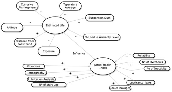
Figure 1.
Asset Health Index, influence diagram.
Figure 2 shows the trends of the Current Health Index (HIc). In other words, the value of the Health Index corrected by the application of the different factors that reflect deterioration in the equipment. The failure rate was calculated for each age of the team using its Weibull parameters from data provided by the organization and summarized in Table 9.
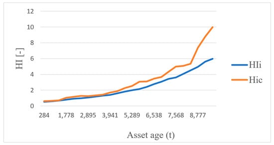
Figure 2.
Initial and Corrected Health Index behavior.
Table 9.
Weibull parameters of the Compressor.
To calculate the corrected failure rate, the Health Correction Factor (k) value was determined for each age of the equipment as described in Equation (10). The corrected failure rate (λ*k) was determined for each age of the equipment with Equation (11). Table 10 shows the values obtained for the Correction Factor (k) and the corrected failure rate (λ*k) for an equipment life cycle, i.e., twenty-four months of operation. The remainder of the LCC computation process is shown in the next section that addresses the sensitivity analysis.
Table 10.
k-factor and corrected failure rate λ*k values.
4. Sensitivity Analysis
The purpose of this section is to validate the LCC model by considering the behavior of the OPEX associated with the operation of the asset over a period of 10 years. For this purpose, and based on the failure rate corrected by the Health Index expressed through the k factor, the costs associated with the Reliability were estimated.
Six hypotheses were put forward for evaluation. With these hypotheses, the aim is to measure the behavior in the total costs due to failures, varying the criteria for carrying out an overhaul. In addition, the case of a simpler (less expensive) and imperfect (not leaving the equipment as good as new) overhaul was also considered. The hypotheses are described below:
Hypothesis 1.
Base case: The overhaul is executed every 9500 operating hours. It returns the equipment to as-good-as-new condition.
Hypothesis 2.
The overhaul is executed every 9500 operating hours. The overhaul is less expensive, but less efficient, and the equipment does not return to its as-good-as-new condition.
Hypothesis 3.
An overhaul is performed when HI = 5.5.
Hypothesis 4.
An overhaul is performed when HI = 4.0.
Hypothesis 5.
An overhaul (cheaper) is performed when HI = 5.5. The overhaul returns the assets to a condition less-than-as-new.
Hypothesis 6.
An overhaul is performed when HI = 4.0. The overhaul is cheaper, but less effective; that is, the equipment does not return to its as-good-as-new condition.
Using Equation (13), the number of failures for each age of the equipment was estimated according to the number of operating hours at each corresponding age, and finally, through Equation (11), the number of annual failures was estimated. Table 11 shows the calculated values.
Table 11.
Obtention of the annual failure rate.
Table 12 summarizes the cost values used to perform a Life Cycle Cost Analysis of the equipment.
Table 12.
Compressor’s Operating costs.
To perform a compressor Life Cycle Cost calculation, a cash flow structure was used in which costs were corrected annually by using an inflation rate. Each of the cost categories must be expressed in present value. In order to compare the obtained results, an analysis of the operational costs (OPEX) of each hypothesis was carried out. Table 13 shows the present value (PV) of the operational costs for each case.
Table 13.
Calculation of annual failures costs.
In the plant under analysis, the compressors are considered as medium critical because the occurrence of failures does not affect the operational continuity of the plant. Therefore, the cost associated with failure events does not include penalties for production unavailability or downtime. Thus, the cost per failure will be associated only with the labor costs of the repair, having consequently a low impact on the total economic calculation. It is based on the aforementioned that the result of Hypothesis 2 can be explained: although the failure rate increases significantly and the number of total failures is almost double of that of the base case, the results are similar. This is because the cost associated with such failures does not exceed the amount of money saved by performing cheaper and less effective overhaul procedures.
Hypothesis 4 gives the highest present value of costs. In this case, by advancing the overhaul, a lower number of failures is estimated; that is, six failures less than the theoretical base case. However, the amount of additional money that will be spent on overhauls is much greater than the money saved due to the lower number of fault events.
Considering Hypothesis No. 3, by anticipating the major maintenance (overhaul) the number of total failures is reduced. However, since the value of failure costs does not have a great impact on the total costs, a result very similar to the base case is obtained.
Hypothesis No. 5 and No. 6 show the lowest values, which is explained by the fact that in both cases the failure rate and consequently the total number of failures is reduced. As the overhaul is considerably advanced, in both hypotheses, the equipment does not reach its aging period and the failure rate will increase only during a short period of infant mortality after each overhaul. Although both hypotheses have a high number of overhauls, the costs associated with these will be lower than the theoretical case because they are less expensive.
5. Comparison with Traditional Model
To demonstrate the impact of failure events on total Life Cycle Costs, it is proposed to compare the results of two of the previously proposed hypotheses with those obtained using a traditional Life Cycle Costing model. Details of each case are described below:
- Case A: Life Cycle Cost Analysis considering a constant failure rate and a Weibull Distribution. The failure frequency function λ is defined by the mean time between failures (MTBF). The required data for this estimation were provided by the organization.
- Case B: Life Cycle Cost Analysis incorporating Asset Health aspects (basic case): costs are estimated considering a variable failure rate based on the ratio of the amount of equipment deterioration to the initial condition, which is quantified by its HI health index. In this case, the overhaul criteria and the quality of the overhaul will be based on data or assumptions provided by the organization.
- Case C: Life Cycle Cost Analysis incorporating Asset Health aspects (overhaul case cheaper and less effective): costs are estimated from a variable failure rate based on the relationship of the amount of equipment deterioration and initial condition, which is quantified by its HI health index. In this case, the overhaul criterion is based on data or assumptions provided by the organization. In addition, and as already mentioned, it is assumed that the overhaul procedure does not return the equipment to its as-good-as-new condition.
Table 14 shows the number of failures per year during the assessment period for the three cases under analysis. As mentioned above, the result of the traditional method uses a constant failure rate over time. The other two cases show a two-year cyclical behavior of the failure rate, a time interval that corresponds to the time between overhauls. The hypothesis of less expensive overhauls shows a higher failure rate over time since in this case the model mimics higher degradation levels of the equipment over time.
Table 14.
Projected annual failures according to traditional method, base case and cheaper overhaul.
Table 15 shows the annual costs considering the reliability behavior and the values adjusted by the inflation rate for each case. In this case, by isolating the costs associated with failure events, the impact of the reliability factor on the economic aspects of the life cycle of an asset can be appreciated. Since the proposed mathematical model aims to incorporate the realistic behavior of the failure rate, it considers the effect of deterioration, the existence of overhaul procedures, the load and operation time. In addition, it takes into account the existence of periods of infant mortality and aging (aspects that the traditional model does not consider). This can be considered a good approximation to achieve a cost estimate with a more conservative view.
Table 15.
Failure event costs.
Figure 3 clearly shows the difference in costs due to low reliability for each year caused by the variation in the failure rate, confirming the hypothesis stated above: by isolating the total costs due to failures, it is possible to appreciate the effect caused by the deterioration processes, among other factors, in the failure rate and consequently the difference in costs, despite the fact that, in this particular case, the Life Cycle Cost is not greatly affected.
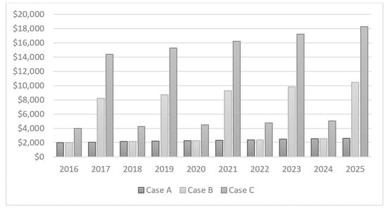
Figure 3.
Costs for reliability; comparison.
6. Conclusions
This paper proposes and experiments with a Life Cycle Costing model based on the adaptation of the Active Health Index methodology. This model is used as the basis for quantifying the deterioration of a complex asset in order to relate its health to the failure rate. Thanks to this, the economic impact of the reliability factor on the life of an asset can be quantified. With this methodology, it was possible to compare and analyze the results obtained by simulating different possible scenarios.
According to the results obtained, it is demonstrated that the model proposed in this study allows a good approximation of the trend of the failure rate based on the Health Index of an asset; in other words, the amount of deterioration of the asset.
In the presented case study, it is shown that, from an economic point of view, the occurrence of fault events does not have the same prominence in the final result as the quantity and quality of the overhauls that are executed. However, in other cases, the occurrence of failure events could have an important impact on the operation of the plant, since possible penalty costs could significantly increase the costs of the failure.
A comparison of the proposed methodology with the traditional method of Life Cycle Costing shows that in the traditional method, failure costs remains constant over the expected useful life, which is considered a limitation in the traditional model. Therefore, the traditional method overlooks important aspects that will affect the real situation and the occurrence of phenomena that influence it (operations, preventive and corrective maintenance, quality of maintenance, etc.).
The methodology proposed in this study is a step forward in the development of Reliability Engineering techniques and in the search for reducing the uncertainty, unawareness and lack of analysis that generate a high cost to companies in the form of unforeseen failures during their operation. The methodology can be applied during the normal operation as well as in design phases with the objective of obtaining the maximum possible profitability in its decision-making and physical asset management processes. One of the outstanding aspects of the methodology is its simplicity of implementation, since it has been applied using a conventional spreadsheet, with the use of some code macros to accomplish certain levels of automation of some processes.
Finally, the analysis of the results obtained in the calculations combined with the result of each simulated scenario constitute a tool with which the company’s technical team can establish decisions related to maintenance planning (preventive, inspections, overhauls, etc.), taking into account the particular conditions of each asset, that is, the impact of each failure event, technical complexity, criticality and maintainability of the equipment, among others.
When forecasting the future states of the Health Modifiers and factors, it incorporates uncertainty into the values defined for each of them. The cognitive map is said to be an apparatus to express the interinfluence of parameters and factors that characterize the dynamics of a system in a given domain. However, these maps have the disadvantage of not being able to handle incomplete or precarious information to represent causal relationships between these parameters. In future works, we shall propose the implementation of fuzzy cognitive maps to better handle the uncertainty or lack of defined information about the states of certain modifiers or factors used to estimate health indices [,].
In the same direction, it is important to bear in mind that the model can be further enhanced by incorporating Monte Carlo simulations to obtain more realistic results. This would require derivation of probability distribution functions for the main cost elements included in the model based on the analysis of existing data.
Author Contributions
Conceptualization, F.O. and O.D.; methodology, O.D.; computations, P.P. and T.H.; formal analysis, O.D.; investigation, O.D.; data curation, F.O.; writing—original draft preparation, O.D.; writing—review and editing, O.D. and F.O.; All authors have read and agreed to the published version of the manuscript.
Funding
This research received no external funding.
Conflicts of Interest
The authors declare no conflict of interest.
References
- International Organization of Standardisation. ISO 55000—Asset Management; International Organization of Standardisation: Vernier, Switzerland, 2014. [Google Scholar]
- van den Honert, A.F.; Schoeman, J.S.; Vlok, P.J. Correlating the content and context of PAS 55 with the ISO 55000 series. S. Afr. J. Ind. Eng. 2013, 24, 24. [Google Scholar] [CrossRef][Green Version]
- Standards Australia. AS/NZS (Standards Australia/Standards New Zealand) 4536 Life Cycle Costing—An Application Guide; Standards Australia: Sydney, Australia, 1999. [Google Scholar]
- International Organization of Standardisation. ISO/IEC/IEEE ISO/IEC/IEEE 15288—International Standard—Systems and Software Engineering—System Life Cycle Processes, 1st ed.; International Organization of Standardisation: Vernier, Switzerland, 2015. [Google Scholar]
- Fabrycky, W.J.; Blanchard, B.S. Life-Cycle Cost and Economic Analysis; Prentice-Hall international series in industrial and systems engineering; Prentice Hall: Upper Saddle River, NJ, USA, 1991. [Google Scholar]
- Kaufman, R.J. Life Cycle Costing: Decision Making Tool For Capital Equipment Acquisitions. J. Purch. 1969, 5, 16–31. [Google Scholar] [CrossRef]
- Hjartarson, T.; Jesus, B.; Hughes, D.T.; Godfrey, R.M. Development of Health Indices for Asset Condition Assessment. In Proceedings of the Proceedings of the IEEE Power Engineering Society Transmission and Distribution Conference, Dallas, TX, USA, 7–12 September 2003. [Google Scholar]
- Hughes, D.T. The use of health indices to determine end of life and estimate remnant life for distribution assets. In Proceedings of the 17th International Conference on Electricity Distribution, Barcelona, Spain, 12–15 May 2003. [Google Scholar]
- Hjartarson, T.; Otal, S. Predicting future asset condition based on current health index and maintenance level. In Proceedings of the Proceedings of the IEEE International Conference on Transmission and Distribution Construction and Live Line Maintenance, ESMO, Albuquerque, NM, USA, 15–19 October 2006. [Google Scholar]
- De la Fuente, A.; Guillén, A.; Crespo, A.; Sola, A.; Gómez, J.; Moreu, P.; Gonzalez-Prida, V. Strategic view of an assets health index for making long-term decisions in different industries. In Proceedings of the Safety and Reliability—Safe Societies in a Changing World—Proceedings of the 28th International European Safety and Reliability Conference, ESREL 2018, Trondheim, Norway, 17–21 June 2018. [Google Scholar]
- Serra, J.; de la Fuente, A.; Crespo, A.; Sola, A.; Guillén, A.; Candón, E.; Martínez-Galan, P. A Model for Lifecycle Cost Calculation Based on Asset Health Index. In Proceedings of the International Conference on Smart Infrastructure and Construction (ICSIC), Cambridge, UK, 8–10 July 2019. [Google Scholar]
- Office of Gas and Electricity Markets. Dno Common Network Asset Indices Methodology; Office of Gas and Electricity Markets: London, UK, 2017.
- Choudhary, M.; Suwanasri, T.; Kumpalavalee, S.; Fuangpian, P.; Suwanasri, C. Condition Assessment of Synchronous Generator Using Fuzzy Logic. IEET 2018, 4, 99. [Google Scholar]
- Nurcahyanto, H.; Nainggolan, J.M.; Ardita, I.M.; Hudaya, C. Analysis of Power Transformer’s Lifetime Using Health Index Transformer Method Based on Artificial Neural Network Modeling. In Proceedings of the International Conference on Electrical Engineering and Informatics 2019, Nanjing, China, 8–10 November 2019. [Google Scholar]
- Aenor. UNE-EN 13306 Maintenance–Terminology 2003; Aenor: Madrid, Spain, 2003. [Google Scholar]
- BSI. BS EN 13306:2010:Maintenance-Maintenance Terminology; BSI: London, UK, 2010; ISBN 978-0-580-64184-8. [Google Scholar]
- Durairaj, S.K.; Ong, S.K.; Nee, A.Y.C.; Tan, R.B.H. Evaluation of life cycle cost analysis methodologies. Corp. Environ. Strateg. 2002, 9, 30–39. [Google Scholar] [CrossRef]
- Woodhouse, J. Turning engineers into businessmen. In Proceedings of the 14th National maintenance conference, London, UK, 1–4 October 1991. [Google Scholar]
- Crespo Márquez, A.; Macchi, M.; Parlikad, A.K. Fundamental Concepts and Framework. In Value Based and Intelligent Asset Management; Springer: Berlin/Heidelberg, Germany, 2020. [Google Scholar]
- Ellram, L.M. Total cost of ownership. Int. J. Phys. Distrib. Logist. Manag. 1995, 25, 4–23. [Google Scholar] [CrossRef]
- Henry, J.; Elfant, C. Cost of ownership. Purch. Manag. 1988, 28, 15–20. [Google Scholar]
- Sheldon, D.F.; Perks, R.; Jackson, M.; Miles, B.L.; Holland, J. Designing for whole life costs at the concept stage. J. Eng. Des. 1990, 1, 131–145. [Google Scholar] [CrossRef]
- Ruparathna, R.; Hewage, K.; Sadiq, R. Multi-period maintenance planning for public buildings: A risk based approach for climate conscious operation. J. Clean. Prod. 2018, 170, 1338–1353. [Google Scholar] [CrossRef]
- Lee, J.; Kim, B.; Ahn, S. Maintenance optimization for repairable deteriorating systems under imperfect preventive maintenance. Mathematics 2019, 7, 716. [Google Scholar] [CrossRef]
- Durán, O.; Afonso, P.S.; Durán, P.A. Spare parts cost management for long-term economic sustainability: Using fuzzy activity based LCC. Sustain. 2019, 11, 1835. [Google Scholar] [CrossRef]
- Woodward, D.G. Life cycle costing—Theory, information acquisition and application. Int. J. Proj. Manag. 1997, 15, 335–344. [Google Scholar] [CrossRef]
- Roda, I.; Macchi, M.; Albanese, S. Building a Total Cost of Ownership model to support manufacturing asset lifecycle management. Prod. Plan. Control 2020, 1–19. [Google Scholar] [CrossRef]
- Cooper, R.; Kaplan, R.S. Profit Priorities from Aotivity-Based Costing. Harv. Bus. Rev. 1991, 69, 130–135. [Google Scholar]
- Cooper, R.; Kaplan, R. Activity-Based Systems: Measuring the costs of resource usage. Account. Horizons 1992, 6, 1–13. [Google Scholar]
- Korpi, E.; Ala-Risku, T. Life cycle costing: A review of published case studies. Manag. Audit. J. 2008, 23, 240–261. [Google Scholar] [CrossRef]
- Crespo Márquez, A.; de la Fuente Carmona, A.; Guillén López, A.J.; Rosique, A.S.; Serra Parajes, J.; Martínez-Galán Fernández, P.; Izquierdo, J. Defining Asset Health Indicators (AHI) to Support Complex Assets Maintenance and Replacement Strategies. A Generic Procedure to Assess Assets Deterioration. In Value Based and Intelligent Asset Management; Springer: Cham, Switzerland, 2020. [Google Scholar]
- Moss, T.R.; Sandtorv, H.; Pratella, C. OREDA Phase II Data Collection Experience. In Reliability Data Collection and Use in Risk and Availability Assessment; Springer: Berlin/Heidelberg, Germany, 1989. [Google Scholar]
- International Organization for Standardization. ISO 20816-1:2016(en), Mechanical Vibration—Measurement and Evaluation of Machine Vibration—Part 1: General Guidelines; International Organization of Standardisation: Vernier, Switzerland, 2016. [Google Scholar]
- International Organization for Standardization. ISO 14830-1:2019 Condition Monitoring and Diagnostics of Machine Systems—Tribology-Based Monitoring and Diagnostics—Part 1: General Requirements and Guidelines 2019; International Organization of Standardisation: Vernier, Switzerland, 2019. [Google Scholar]
- Falcone, P.M.; De Rosa, S.P. Use of fuzzy cognitive maps to develop policy strategies for the optimization of municipal waste management: A case study of the land of fires (Italy). Land Use Policy 2020, 96, 104680. [Google Scholar] [CrossRef]
- Kokkinos, K.; Karayannis, V.; Moustakas, K. Circular bio-economy via energy transition supported by Fuzzy Cognitive Map modeling towards sustainable low-carbon environment. Sci. Total Environ. 2020, 721, 137754. [Google Scholar] [CrossRef] [PubMed]
Publisher’s Note: MDPI stays neutral with regard to jurisdictional claims in published maps and institutional affiliations. |
© 2020 by the authors. Licensee MDPI, Basel, Switzerland. This article is an open access article distributed under the terms and conditions of the Creative Commons Attribution (CC BY) license (http://creativecommons.org/licenses/by/4.0/).