1. Introduction
Partial differential equations (PDEs) have a vital role in describing different phenomena in real life. Such applications appear in many fields—in industry, biology, agriculture, petro-chemistry, heat transfer in draining films, the spread of solutes in liquid flowing through a tube, flow in porous media, meteorology and electric discharge [
1,
2,
3,
4,
5,
6]. Fluid dynamics is an important scientific area where governing equations are most often differential equations, and any analytical solutions for these equations are only possible for a restricted and limited number of cases. Due to this, several numerical techniques have been developed for the numerical approximations of convection–diffusion problems [
7,
8,
9,
10,
11,
12,
13,
14,
15,
16,
17,
18]. The most common numerical techniques are based on the finite difference method, the finite volume method and the finite element method. The comparison of finite difference and finite volume method for the numerical approximation of the convection–diffusion equation was studied in the papers [
19,
20,
21,
22]. The finite volume method is a special kind of numerical approach which is widely used for solving convection–diffusion problems in computational fluid dynamics [
23,
24,
25,
26,
27] and also to simulate advection-diffusion problems with convection dominated processes [
28,
29,
30]. The numerical simulation and the error estimate of steady-state convection–dominated diffusion problem was investigated in [
31] using a cell-vertex finite volume approximation, whereas [
32] used cell-centered finite difference approximations for a steady-state convection–diffusion problem to get second-order convergence that fulfilled the discrete maximum principle with discrete Sobolev spaces. By looking at the work in [
33] a singular perturbed convection–diffusion problem was discretized with the help of the upwind finite volume scheme with uniform point-wise convergence over layer-adapted meshes. The authors [
34] discussed the numerical solution of the unsteady-state advection-diffusion problem in two dimensions using the upwind finite volume method and an alternating-implicit, upwind finite volume method. Numerical simulations of non-Newtonian fluids were investigated using the finite volume formulation [
35], where the approximation of the convection process is managed by using the QUICK differences scheme. A two-dimensional, incompressible in-viscid-free surface was simulated in [
36] and they used the level set method for capturing the interface. A numerical solution of the convection–diffusion problem with variable coefficients over the nonstandard control volume grid was analyzed in [
37] using the weighted upwind finite volume method. In the [
38] finite volume method combined with the Lattice–Boltzmann method was studied for discretizing the convection operator over different regions, whereas [
39] discussed the error estimation of the non-linear advection operator using the upwind finite volume method over a geometric corrector. In the meantime, the convergence analysis for the general initial and boundary condition with linear transport problems over the regularity property was solved in [
40] using the upwind finite volume method.
Since in flow simulations it is imperative to satisfy conservation laws at all levels [
41], by avoiding generation and consumption of mass, energy and momentum due to artificial terms inside the control volume, this is not guaranteed in finite difference and finite element methods. The control volume integration is a key step in the finite volume method, which ensures the conservation of relevant properties at each finite control cell level. This control volume integration gives a semi–discretize conservation law which involves fluxes at the interfaces of control volumes. The most popular forms of the finite volume method discretization are cell-centered, vertex-centered and face-centered [
42]. The important contributions of the finite volume method are that it can also be formulated in the physical space on unstructured meshes and it is relatively easy to implement a variety of boundary conditions in a non-invasive manner [
43].
The numerical schemes for time-dependent problems are known as explicit, implicit and fully implicit based on the chosen temporal approximation. One of the most common and widely used techniques for temporal approximation is the Crank–Nicolson method [
44,
45]. This technique forms a second-order implicit scheme in time. John Crank and Phyllis Nicolson constructed this well-known numerical technique in the mid 20th century [
44,
46,
47,
48,
49,
50,
51]. In the past, based on spatial interface approximations, several finite volume numerical schemes were developed to solve the convection–diffusion problem.
In this study, based on the upwind approach, new expressions were obtained for spatial approximation at the interface. Crank–Nicolson formulation is used for the approximation along the temporal direction, and using these new interface approximations, a numerical scheme was developed for the numerical approximation of convection–diffusion problem. This newly developed scheme is unconditionally stable and gives second-order accuracy. Some numerical experiments have been carried out to validate our newly developed theoretical algorithm for the upwind approach, and we have compared the numerical results of our modified upwind approach with the central differences scheme and the most common upwind approach [
4,
21], and the numerical approximation of the unsteady convection–diffusion problem.
The paper is organized as follows: we have introduced preliminary remarks and definitions in
Section 2. We have also shown the discretized and formulated form of our problem in
Section 3, and in
Section 4, the numerical scheme is treated and analyzed with the boundary condition. In addition, our stability and convergence order analysis are discussed using the von Neumann–Fourier method in
Section 5. In
Section 6, numerical experiments are shown to verify our theoretical study and the conclusions are presented in
Section 7.
3. Discretization and Formulation of the Problem
The convection–diffusion equation can be either convection or diffusion dominated; it depends on the rate of convection and the rate of diffusion. The impact of convection on the transport of physical quantity is measured by Reynold number or the local Peclet number
. For the discretization we have used the domains
and
. Consider the one-dimensional convection–diffusion equation with constant coefficients:
with initial condition
and boundary condition
where
represent the convective velocity and diffusion coefficient respectively, whereas
is the variable convected in x-direction.
and
are called convective (sometimes advective) and diffusive (sometimes viscous) terms respectively. For easy implementation of the new upwind approach of the finite volume method, we do not consider the source/sink term in our discretization of the Equation (
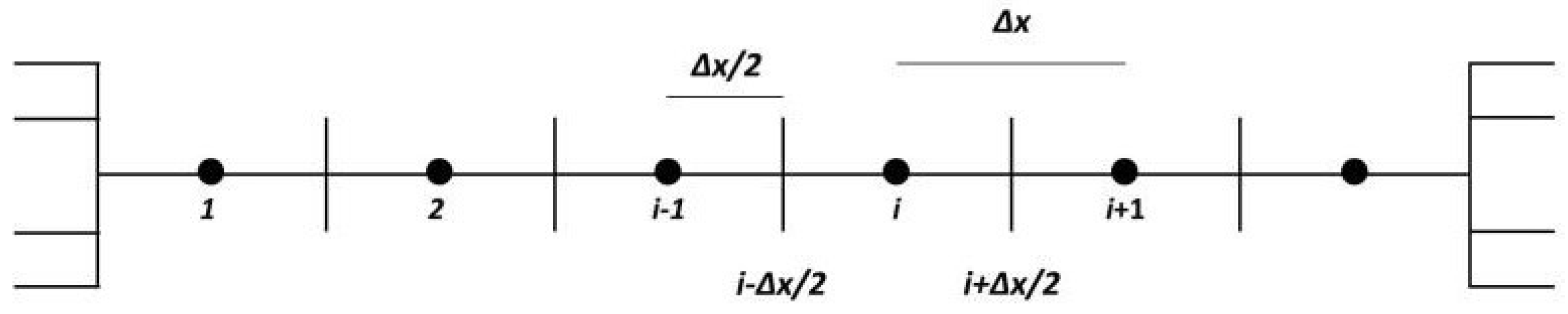
1). The term convection means the movement of molecules within the fluid. In contrast, diffusion describes the spread of particles through the random motion from the region of high concentration to lower concentration region. In problems in which fluid flow plays important roles, we must consider the effects of convection dominance. A uniform discretization of the finite volume method is shown in
Figure 2.
By integrating the problem over the control volume,
around the nodal point
i.
Here, the first term will be approximated by using trapezoidal rule for numerical integration
Here we need to make an approximation of variable and its gradients at the interface, as gradients will be approximated using central difference approximation as
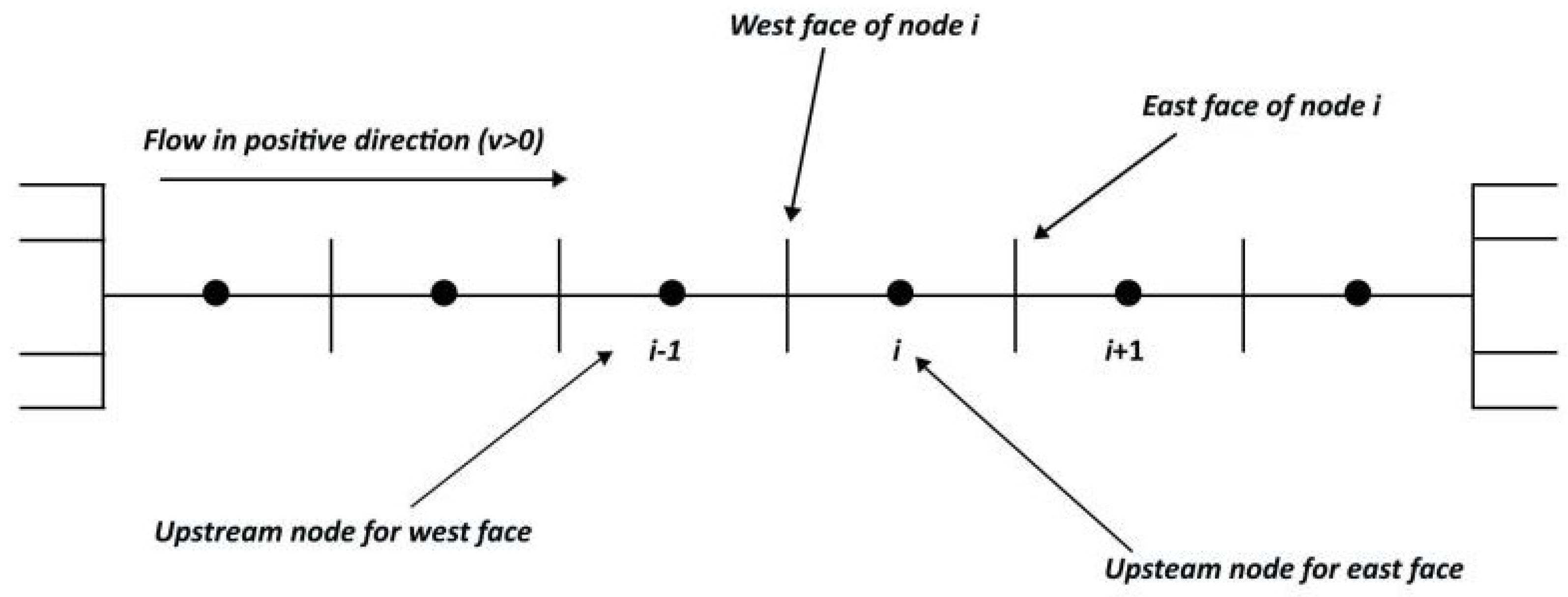
Remark 2. One of the major inadequacies of the central difference scheme is its inability to identify the flow direction while approximating these interface fluxes. This scheme treats equally (taking the average value) both neighbor nodes of any interface when approximating the variable at interface, whereas the existing and commonly used upwind approach considers the flow direction with the first-order accuracy. In the current study a numerical scheme based on upwind approach is proposed with second-order accuracy.
For an upwind approach, The upstream or high influential node for each interface of
ith control volume is indicated in
Figure 1. In the case of the upwind approach (
) the flow is coming from the left side and approximates at its east face
in terms of its upstream node
will be:
Here
can be approximated by using the central difference approximation between the nodes
and
as follows:
By putting this approximation in the above Equation (
5), we have:
This Equation (
6), shows our expression for east interface
approximation based on the upwind approach (
). Now for the upwind approach (
) the west face
will be approximated by its upstream node
:
Here
can be approximated by central difference scheme approximation between the node
and
as follows:
Substitute this approximation into (
7) and it becomes:
This Equation (
8) shows our approximation at the west interface
of the
ith control volume when (
). Now substitute the approximations given in Equations (
3), (
4), (
6) and (
8) in above semi-discretized Equation (
2); we get:
After some simplification we get:
After some rearrangements, the above expression becomes:
Here
method is used to evaluate the temporal integration:
where
For the Crank–Nicolson scheme
=
and also divide by
This Equation (
13) shows our numerical scheme based on the upwind approach of the finite volume method, and it is valid for interior nodes from node 3 to
with the convergence of second-order in both space and time. For
and
this scheme gives
,
and
which we do not have in our computational domain; such cells are called ghost cells and values for these cells are called ghost values. For the special treatment of these boundary nodes (see in
Section 4), our modified scheme holds the property of boundedness and also ensures the conservation of the variable using the consistent and same approximation expressions for a common interface of the two adjacent control volumes.
Remark 3. For a downwind approach also we have define the upstream nodes (see Definition 2) and in the case of the downwind approach, i.e., , our interface approximations will be With these interface approximations for the downwind approach the numerical scheme will be 4. The Formulation of the Problem within the Analysis of Boundary Conditions
The boundary nodes 1, 2 and n need special treatment for the discretization of a governing equation over these nodes.
For node 1 the wet face
is known because it coincides with the left boundary of the physical domain.
The east face of node 1
can be approximate from Equation (
6) by taking
. For the approximation of east face of node 1 we have adjusted an imaginary node
outside the boundary of the domain at a distance
(see in Remark 1 and
Figure 3). For east face of node 1, Equation (
6) becomes
Here
is our left imaginary node; substitute its approximated value (see Remark 1) in Equation (
15)
This expression (
16) shows the east face approximation of node 1. By substituting the approximations in expression (
14) and (
16) into Equation (
2), the discretized equation for node 1 will be
This is the discretized equation for node 1. As the uniqueness and major advantage of the finite volume method is to ensure the conservation of variable by using the consistent expression for a common interface between two adjacent control volumes, the west face of node 2 and east face of node 1 must have same approximation expression:
The east face of node 2 can be approximated from expression (
6) by taking
.
Using the expressions (
18) and (
19) for west and east face approximations of node 2 respectively, the expression (
2) after some simplification and applying the
method gives the discretized equation for node 2 as
This is the final discretized equation for node 2. The upstream node for east face
is node n and can by approximated form expression (
6) by taking
:
is our right side imaginary node (see
Figure 3); put the approximation of imaginary node
(see Remark 1) in Equation (
21) and it becomes
is known because it lies over the right boundary of physical domain. The west face
can be approximated using Equation (
8) by taking
:
By using the Equations (
22) and (
23) for node n the discretized equation will be
6. Numerical Experiments
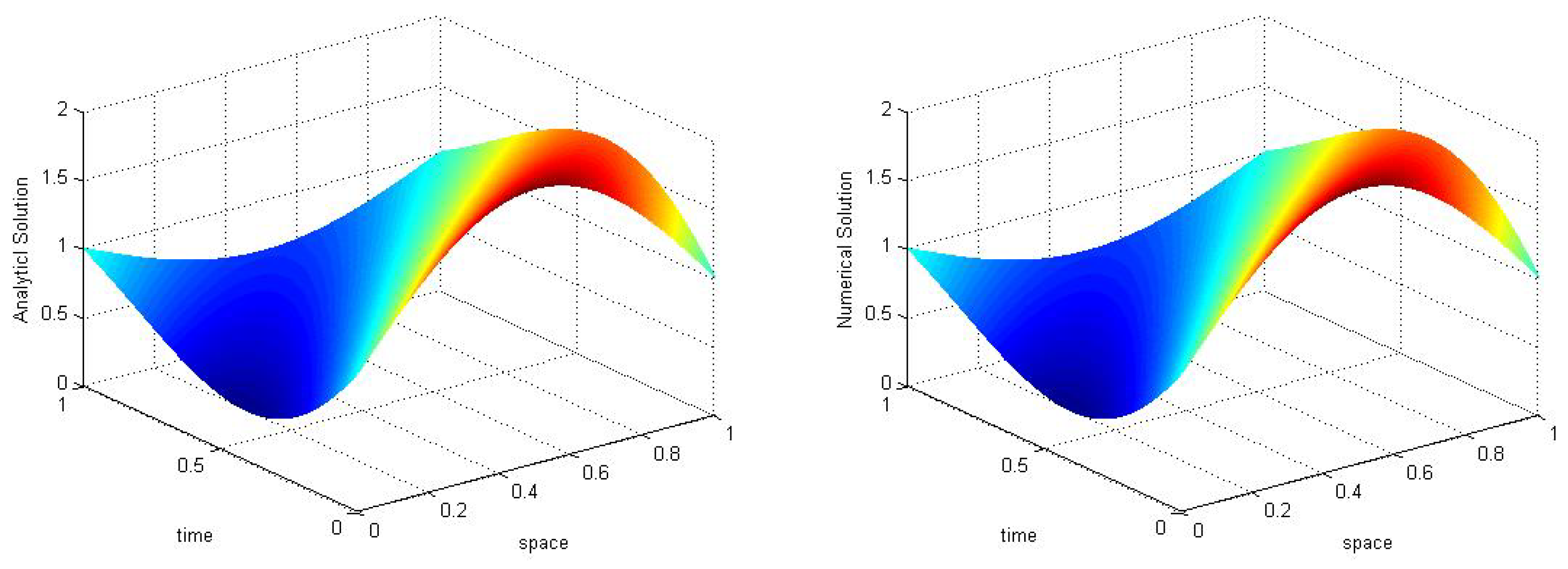
1. Let
be the property transported by means of convection and diffusion processes through one dimensional domain. Using equally spaced cells with the modified scheme of the finite volume method for the convection–diffusion equation, calculate the distribution of
. The analytical solution of the problem given in [
15] by
is considered on the finite domain
. The initial and boundary values are calculated from the exact solution by taking
and
, respectively.
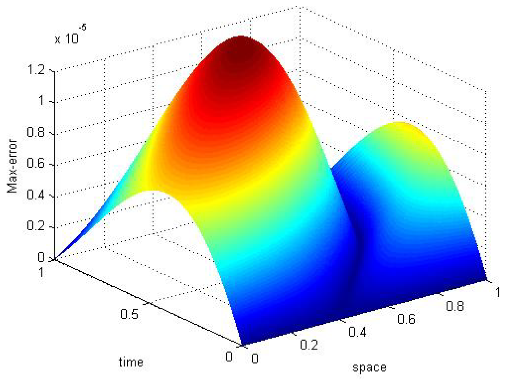
For time step
and spatial step size
the convection–diffusion problem is solved using a modified upwind approach of the finite volume method, obtaining numerical solution and maximum are shown in
Figure 4.
The spatial and temporal convergence order of the newly constructed scheme are displayed in
Table 1 and
Table 2, respectively. In
Table 1 spatial convergence has been proved for temporal step sizes
and
, whereas spatial step size
taken as
and
. In
Table 2 results for the temporal convergence order have been shown. Temporal convergence order is proved for spatial step size (
) taken as
and
,;the temporal step size (
) is
or
. The obtained spatial and temporal convergence order mentioned in
Table 1 and
Table 2 supports our theoretical approach about the convergence order of our scheme (see
Section 3 and
Section 5.2).
2. Consider a homogeneous one dimensional convection–diffusion problem over a computational domain,
; its exact solution is given in [
16] as:
with
as the convection velocity to the
direction and
as the diffusion coefficient. Now, we can find the transported property
for two different cases of convection dominance and diffusion dominance respectively, using the modified upwind finite volume method with equally spaced cells. The initial and boundary values are calculated from an exact solution by taking
and
, respectively.
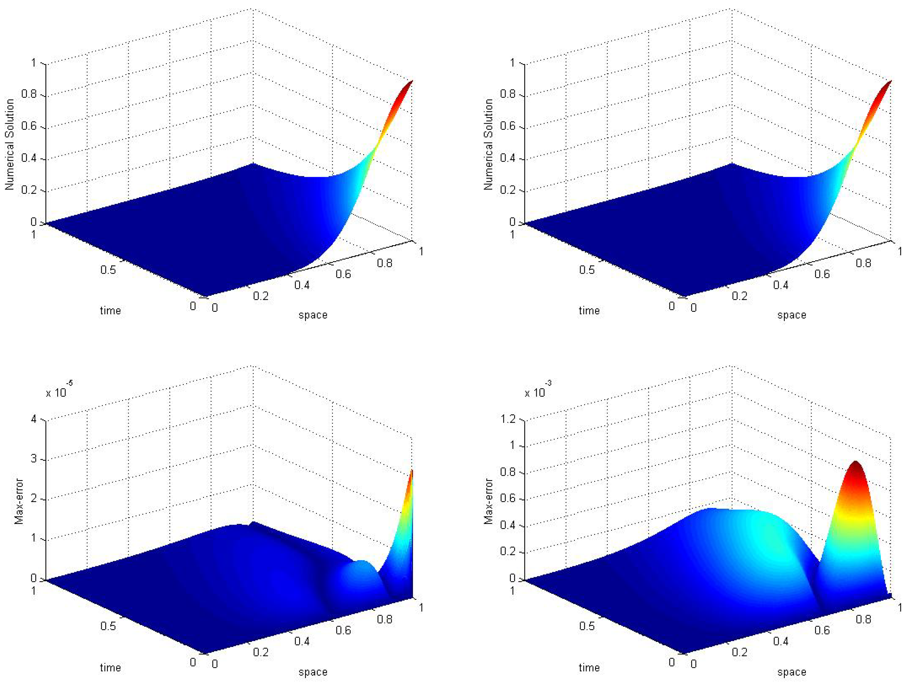
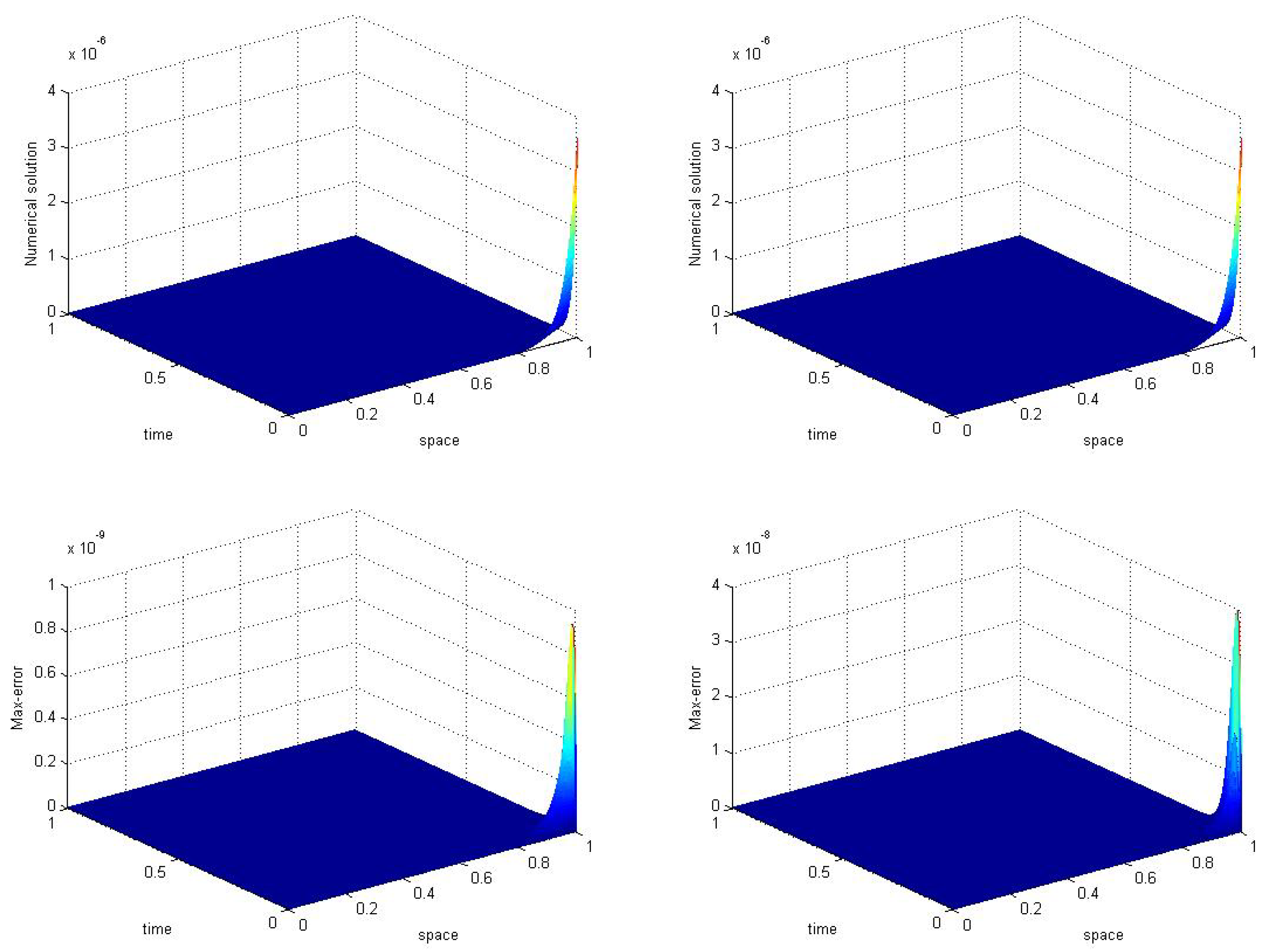
In
Figure 5 numerical results for the convection dominant case (
) are expressed. The left figures show the numerical approximation and maximum error of the modified upwind finite volume method. In contrast, figures on the right side represent the numerical solution and maximum error using an existing upwind finite volume method for the convection–diffusion problem. In this case, the numerical value of maximum error produced by the new upwind scheme was 3.1930 ×
, but for the existing upwind scheme, the maximum error was
. This indicates new upwind scheme has the ability to deal with a dominant convection problem numerically as compared to the existing upwind scheme, and this shows consistency with our theoretical approach.
Table 3 and
Table 4 respectively show the maximum errors with spatial convergence order and temporal convergence order respectively, for the new scheme and existing upwind scheme of finite volume method. The spatial order of convergence in the case of convection dominance (
k = 0.4 and
v = 1) has been proven for temporal step sizes
1/5000 and 1/10,000. For temporal convergence order, spatial discretization width
is taken as
and
. The results shown in both tables support to our theoretical algorithm.
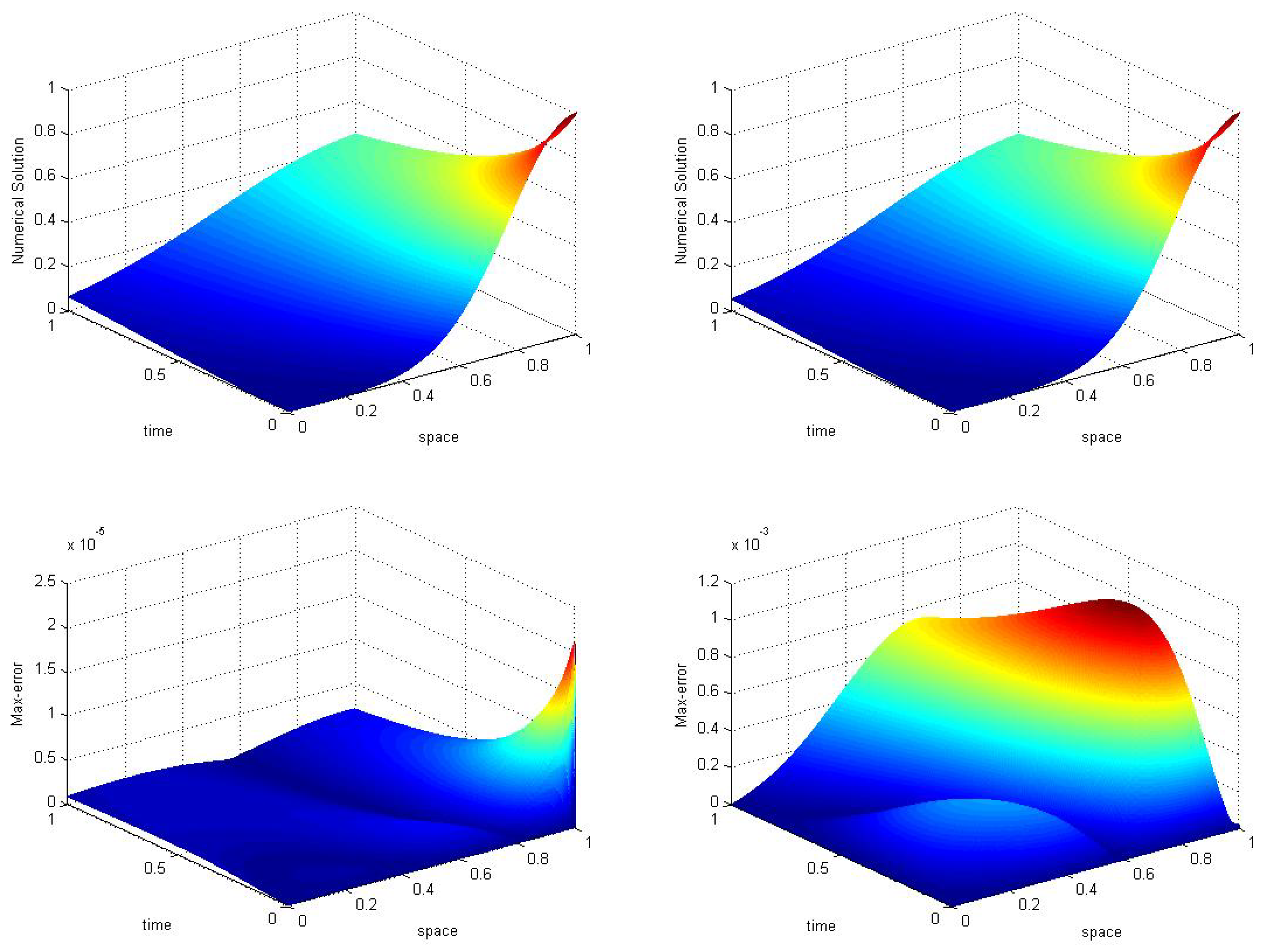
In
Figure 6 numerical results for the diffusion dominant case
are expressed. Left figures show the numerical approximation and maximum error of the modified upwind finite volume method. In contrast, figures at the right side represent the numerical solution and maximum error using an existing upwind finite volume method for the convection–diffusion problem. In this case, the numerical value of maximum error produced by the new upwind scheme is
, but for the existing upwind scheme, it is
. This implies that for a dominant diffusion problem, the new upwind scheme gives a higher accuracy solution than the existing upwind FVM.
Table 5 and
Table 6 respectively show the maximum error with spatial convergence order and temporal convergence order for the new numerical scheme and existing upwind scheme of finite volume method in the case of diffusion dominance. To prove the spatial and temporal convergence order in case of diffusion dominance, coefficients are taken as
and
. For temporal convergence, the numbers of spatial nodes are taken as
and 400. For spatial convergence, time level
is fixed at
and 10,000. The results shown in both tables support to our theoretical algorithm. From both tables it is clear that the new upwind scheme gives less maximum error; this implies that the numerical approximation is highly accurate as compared to the existing numerical scheme.
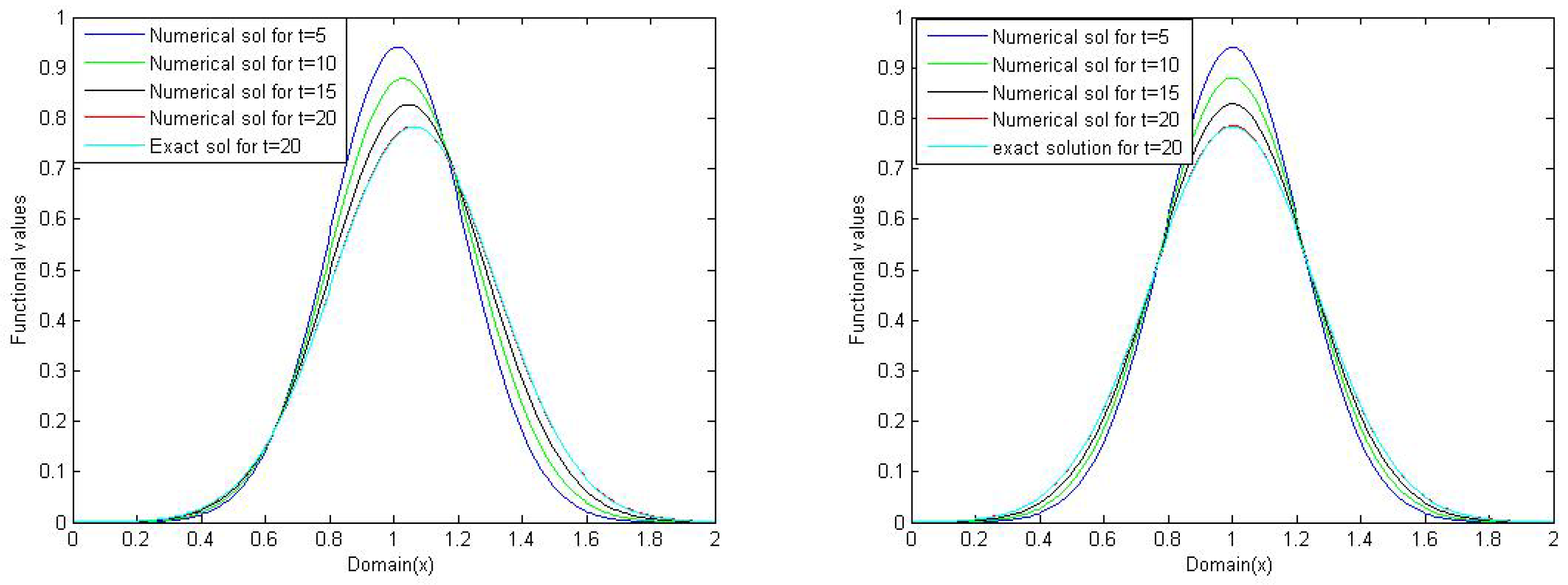
Figure 7 shows the numerical approximation (for numerical example 2) of the convection–diffusion problem using the modified upwind finite volume method with different time levels. Numerically, we have tested the modified scheme for convection dominance (see left of
Figure 7) and for diffusion dominance (see right of
Figure 7). Both figures indicate that the increase of the time level for a numerical solution using our proposed numerical scheme get closeness to an exact solution.
3. Consider a homogeneous one dimensional convection–diffusion problem over a computational domain,
where its exact solution is given in [
16] as:
with
is the convection velocity to the
direction and
is the diffusion coefficient. Now, we can find the transported property
for two different cases of convection dominance using new upwind finite volume method with equally spaced cells. The initial and boundary values are calculated from the exact solution by taking
and
, respectively. We took time step
and spatial step size
. This numerical experiment also shows a numerical comparison of the modified finite volume method and the most common form (central difference scheme) of finite volume method for the approximation of the convection–diffusion problem.
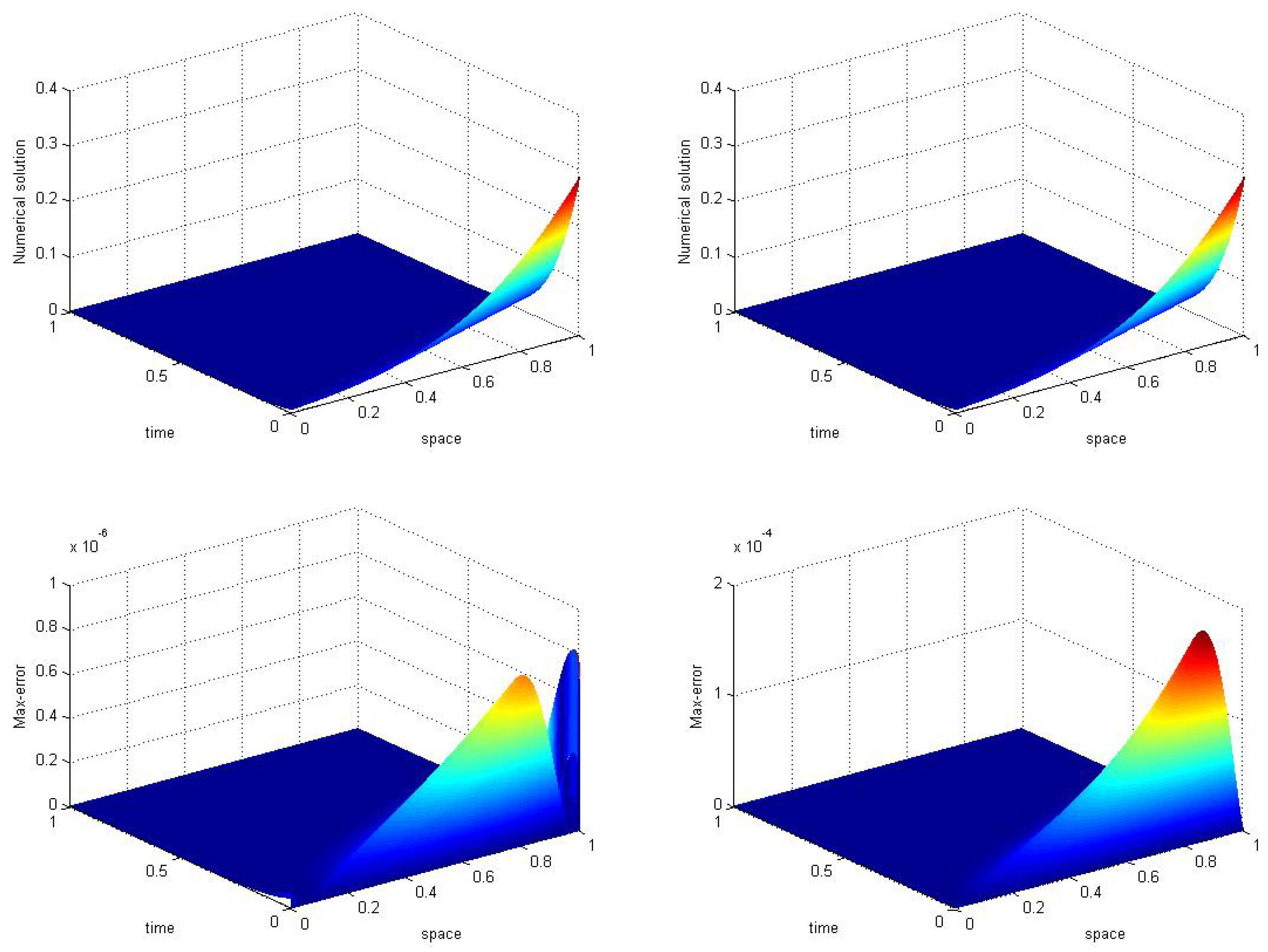
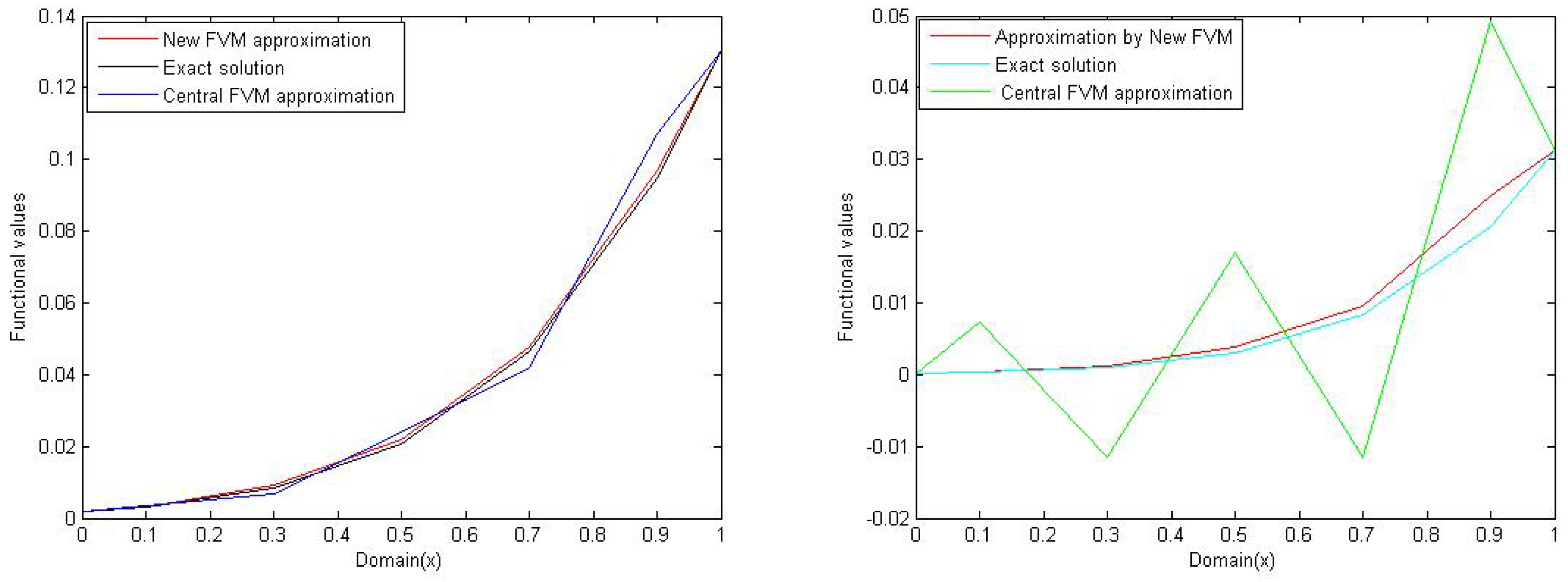
In
Figure 8 and
Figure 9 numerical approximations using new form of finite volume method and the most central difference scheme of FVM are compared for different cases of convection dominance. When we compare the max-errors of both numerical schemes, in the first case (when
and
) the max-errors produced by new FVM scheme and central (FVM) scheme are
and
respectively. For the second convection dominance case (
) the new scheme gives max-error
and the central scheme gives
. This implies that, for both cases, this newly constructed FVM scheme gives highly accurate results and it has the good capability to deal with convection dominance as compared to the central scheme of finite volume method.
Figure 10 shows the numerical behavior of both numerical schemes for different values of the Peclet number (
).
Figure 10 left and right express the results for
and
respectively. From both figures, it is clear that the central difference scheme produces a solution that appears to oscillate about the exact solution. These oscillations are often called “wiggles” in the literature. The consistency with the analytical solution is weak as compared to the modified scheme of finite volume method.


