Spurious OLS Estimators of Detrending Method by Adding a Linear Trend in Difference-Stationary Processes—A Mathematical Proof and Its Verification by Simulation

Abstract

Adding a linear trend in regressions is a frequent detrending method in economic literatures. The traditional literatures pointed out that if the variable considered is a difference-stationary process, then it will artificially create pseudo-periodicity in the residuals. In this paper, we further show that the real problem might be more serious. As the Ordinary Least Squares (OLS) estimators themselves are of such a detrending method is spurious. The first part provides a mathematical proof with Chebyshev’s inequality and Sims–Stock–Watson’s algorithm to show that the OLS estimator of trend converges toward zero in probability, and the other OLS estimator diverges when the sample size tends to infinity. The second part designs Monte Carlo simulations with a sample size of 1,000,000 as an approximation of infinity. The seed values used are the true random numbers generated by a hardware random number generator in order to avoid the pseudo-randomness of random numbers given by software. This paper repeats the experiment 100 times, and gets consistent results with mathematical proof. The last part provides a brief discussion of detrending strategies.

1. Introducing the Problematic

The traditional time-series models focused on stationary processes. As a matter of fact, Wold’s (1954) [1] famous decomposition theorem indicated that any covariance-stationary process could be formulated as the sum of infinite white noises. Thanks to this stationary process’ property, the Autoregressive moving average model (ARMA) models applying the method proposed by Box and Jenkins (1970) [2] gradually became the main modeling in time-series analysis. However, what happens when the series are not stationary?

By simulating two distinct random walks and regressing one to another, Granger and Newbold (1974) [3] revealed the “spurious regression problem.” The OLS estimators of the correlation between these two independent random walks should be zero, but the Monte Carlo simulations performed by the econometricians indicated OLS estimators significantly different from zero, along with very high R². They put forward the idea that such a regression is “spurious,” because it makes no sense, even when it exhibits very high R². Other authors, such as Phillips (1986) [4] or Davidson and McKinnon (1993) [5], revealed similar results, leading to the following conclusions: (i) If the dependent variable is integrated of order 1, that is to say, I(1), then under null hypothesis, the residuals of the regression would also be I(1). However, as the usual statistical tests of the OLS estimators (Fisher or Student tests) are based on a hypothesis of residuals as white noise, these tests are no longer effective if such an assumption is not maintained. (ii) Some asymptotic properties are no longer valid, such as those of the ADF statistics, because they did not obey the same laws in the case of stationary processes. (iii) As the residuals are also I(1), the previsions are not efficient—except when a cointegration relationship between variables exists.

Here, we only examine time-series nonstationarity on average, to be distinguished from that in variance. Since Nelson and Plosser’s (1982) [6] contribution, nonstationarity on average can itself be classified into two categories: the first one is related to trend-stationary (TS) processes which present nonstationarity because of the deterministic trends characterizing their structure; the second category is linked to difference-stationary (DS) processes which contain a stochastic structure, or unit root. The processes considered can be made stationary by adding or removing the deterministic trends in the regressions in the case of TS processes, or, alternatively, in the case of DS processes, through difference operators, going from ARMA to Autoregressive Integrated Moving Average model (ARIMA).

Unit root tests are generally used to identify the nature of a nonstationary process, whether deterministic or stochastic. For DS, in particular, a solution is offered within ARIMA models through difference operators or the cointegration methods respectively proposed by Engle and Granger (1987) [7] in a univariate approach, and by Johansen (1991) [8] in a multivariate approach. Meanwhile, Stock (1987) [9] has demonstrated that, within such frameworks, the OLS estimators converge toward the real values if the variables are cointegrated, and the speed of convergence is faster than that of the usual case (that is, 1/T instead of 1/$\surd T$, where T is the sample size).

The cointegration theory achieved great success, but it has several inconveniences. It requires that all the variables must be integrated in the same order; otherwise, the cointegration models cannot be applied. However, it is difficult to make sure that all series have the same order of integration in the economic model which is tested. For example, GDP growth rates are often I(0), while some price indices can be I(2). Moreover, a supplementary difficulty in using difference operators destined to stabilize a DS process comes from the fact that variables in various orders of difference may not match the theoretical models which are employed.

It follows that the detrending method consisting of adding a linear trend into the regression has become common in empirical studies, due to its simplicity and its compatibility with a wide range of models. Many authors have chosen to add a linear trend in their regressions when they considered their dependent variables as nonstationary. Thus, detrending methods are often used in TS processes despite the nonstationary nature of the latter. Nevertheless, TS detrending methods cause specific problems when the series is in fact a DS process.

2. Literature Review

Studying the implications of treating TS processes as DS processes with the application of a difference operator, Chan, Hayya and Ord (1977) [10] found that the difference operator creates an artificial disturbance in the differentiated series. Indeed, the autocorrelation function equals to −1/2 when lag = $\pm 1$. Later, Nelson and Kang (1981) [11] examined the reverse case, in other words, the effects of treating DS processes as TS processes by adding a linear trend into the regression, and stated that, when a detrending method is used, the covariance of the residuals depends on the size of the sample and on time. By simulation, they showed that adding a linear trend into the regressions for TS processes generates a strong artificial autocorrelation of the residuals for the first lags, and thus induces a pseudo-periodicity—the corresponding spectral density function exhibiting a single peak at a period equal to 0.83 of the sample size. More precisely, treating TS processes as DS processes by difference operator artificially creates a “short-run” cyclical movement in the series, while, conversely, a “long-run” cyclical movement is artificially generated when treating DS processes as TS processes (we speak about “short-run,” since the disturbance happens when lag = $\pm 1$, and “long-run,” because the problem appears when the period corresponds to 0.83 of the sample size, or almost the same importance than the latter).

These fundamental studies have shown the importance of distinguishing between TS and DS processes, but remained concentrated on artificial correlations of the residuals. None of them focused on the OLS estimators themselves. In addition, the samples which are used are relative small. Following Nelson and Kang’s (1981) [11] research line, we shall mathematically demonstrate that the OLS estimators of detrending method by adding a linear trend in DS processes can be considered as spurious. As we shall see, the OLS estimator of the trend tends to zero when the sample size tends to infinity, while the other OLS estimator (intercept) is divergent in the same situation. After this, we shall design a simulation series to be experimented on by a sample of a million observations. The seed values are given by Rand Corporation (2001) [12]. As the dataset of simulation contains more than 100 million points, we shall present the program built by SAS with the seed values table in the Appendix A, so that readers will be in a position to reproduce the simulations with the same codifications.

3. A Mathematical Proof

We suppose that $y_t$ is a DS; for example, the random walk:

$$y_t=y_{t-1}+v_t$$

where $v_t$ is a white noise—and considering a weak form of stationarity, or of the second order.

Let us apply a time detrending method by adding a linear trend into the regression; that is to say, we have the model:

$$y_t=\alpha +\beta t+{\epsilon }_t$$

where $\alpha$ and $\beta$ are coefficients to be estimated, and t is the time variable: t = 1,2,3…T, with T the sample size, or number of observations. ${\epsilon }_t$ is the innovation.

Suppose: $X_t=\left(\begin{array}{c}1\\ t\end{array}\right)$, $\gamma =\left(\begin{array}{c}\alpha \\ \beta \end{array}\right)$, and $b_T$ is the OLS estimators of $\gamma$ based on a sample of size T.

We get:

$$b_T=\left(\begin{array}{c}\widehat{{\alpha }_T}\\ \widehat{{\beta }_T}\end{array}\right)={\left({\displaystyle \sum }_{t=1}^T{X}_t{X}_t^{\prime }\right)}^{-1}\left({\displaystyle \sum }_{t=1}^T{X}_t{y}_t\right)$$

For the term:

$$\left({\displaystyle \sum }_{t=1}^T{X}_t{X}_t^{\prime }\right)=\left(\begin{array}{cc}{{\displaystyle \sum }}^{ }1& {{\displaystyle \sum }}^{ }t\\ {{\displaystyle \sum }}^{ }t& {{\displaystyle \sum }}^{ }{t}^2\end{array}\right)=\left(\begin{array}{cc}T& T\left(T+1\right)/2\\ T\left(T+1\right)/2& T\left(T+1\right)\left(2T+1\right)/6\end{array}\right)$$

As

$${\left(\begin{array}{cc}a& b\\ c& d\end{array}\right)}^{-1}=\frac{1}{ad-bc}\left(\begin{array}{cc}d& -b\\ -c& a\end{array}\right)$$

Then:

$$\begin{gathered} {\left({\displaystyle \sum }_{t=1}^T{X}_t{X}_t^{\prime }\right)}^{-1}=\frac{1}{T^2\left(T+1\right)\left(2T+1\right)/6-T^2{\left(T+1\right)}^2/4}\left(\begin{array}{cc}T\left(T+1\right)\left(2T+1\right)/6& -T\left(T+1\right)/2\\ -T\left(T+1\right)/2& T\end{array}\right) \\ =\frac{12}{T^2\left(T+1\right)\left(T-1\right)}\left(\begin{array}{cc}\frac{T\left(T+1\right)\left(2T+1\right)}{6}& -\frac{T\left(T+1\right)}{2}\\ -\frac{T\left(T+1\right)}{2}& T\end{array}\right) \\ =\frac{2}{T\left(T-1\right)}\left(\begin{array}{cc}2T+1& -3\\ -3& 6/\left(T+1\right)\end{array}\right) \end{gathered}$$

Additionally, for the term:

$$\left({\displaystyle \sum }_{t=1}^T{X}_t{y}_t\right)=\left(\begin{array}{c}{\displaystyle {\displaystyle \sum }_{t=1}^T}{y}_t\\ {\displaystyle {\displaystyle \sum }_{t=1}^T}t{y}_t\end{array}\right)$$

So:

$$\begin{array}{cc}\hfill \left(\begin{array}{c}\widehat{{\alpha }_T}\\ \widehat{{\beta }_T}\end{array}\right)=& \frac{2}{T\left(T-1\right)}\left(\begin{array}{cc}2T+1& -3\\ -3& 6/\left(T+1\right)\end{array}\right)\left(\begin{array}{c}{\displaystyle {\displaystyle \sum }_{t=1}^T}{y}_t\\ {\displaystyle {\displaystyle \sum }_{t=1}^T}t{y}_t\end{array}\right)\hfill \\ \hfill =& \frac{2}{T\left(T-1\right)}\left(\begin{array}{c}\left(2T+1\right){{\displaystyle \sum }}^{ }{y}_t-3{{\displaystyle \sum }}^{ }t{y}_t\\ -3{{\displaystyle \sum }}^{ }{y}_t+\frac{6}{T+1}{{\displaystyle \sum }}^{ }t{y}_t\end{array}\right)\hfill \end{array}$$

Thus, we have, respectively:

$$\{\begin{array}{c}\widehat{{\alpha }_T}=\frac{2}{T\left(T-1\right)}\left(\left(2T+1\right){{\displaystyle \sum }}^{ }{y}_t-3{{\displaystyle \sum }}^{ }t{y}_t\right)\\ \widehat{{\beta }_T}=\frac{6}{T\left(T-1\right)}\left(-{{\displaystyle \sum }}^{ }{y}_t+\frac{2}{T+1}{{\displaystyle \sum }}^{ }t{y}_t\right)\end{array}\left(A\right)$$

However, initially we have seen that:

$$y_t=y_{t-1}+v_t$$

Additionally

$$v_t~WN$$

That is:

$$y_t=y_0+{\displaystyle \sum }_{j=1}^t{v}_j$$

Therefore:

$$\begin{gathered} {\displaystyle \sum }_{t=1}^T{y}_t={\displaystyle \sum }_{t=1}^T\left(y_0+{\displaystyle \sum }_{j=1}^t{v}_j\right)=T{y}_0+T{v}_1+\left(t-1\right)v_2+\cdots +2v_{T-2}+v_T \\ =T{y}_0+{\displaystyle \sum }_{t=1}^T\left(T+1-t\right)v_t=T{y}_0+\left(T+1\right){\displaystyle \sum }_{t=1}^T{v}_t-{\displaystyle \sum }_{t=1}^{T}t{v}_t \end{gathered}$$

Additionally:

$$\begin{gathered} {\displaystyle \sum }_{t=1}^{T}t{y}_t={\displaystyle \sum }_{t=1}^{T}t\left(y_0+{\displaystyle \sum }_{j=1}^t{v}_j\right)=y_0{\displaystyle \sum }_{t=1}^{T}t+{\displaystyle \sum }_{t=1}^{T}t\left({\displaystyle \sum }_{j=1}^t{v}_j\right) \\ =y_0\frac{\left(T+1\right)T}{2}+\left(1+\cdots +T\right)v_1+\left(2+\cdots +T\right)v_2+\cdots +\left(T-1+T\right)v_{T-2}+T{v}_T \\ =y_0\frac{\left(T+1\right)T}{2}+{\displaystyle \sum }_{t=1}^T\frac{\left(t+T\right)\left(T-t+1\right)}{2} =y_0\frac{\left(T+1\right)T}{2}+\frac{T\left(T+1\right)}{2}{\displaystyle \sum }_{t=1}^T{v}_t-\frac{1}{2}{\displaystyle \sum }_{t=1}^T{t}^2{v}_t+\frac{1}{2}{\displaystyle \sum }_{t=1}^{T}t{v}_t \end{gathered}$$

It becomes:

$$\widehat{{\alpha }_T}=y_0+\frac{\left(T+1\right)\left(T+2\right)}{\left(T-1\right)T}{\displaystyle \sum }_{t=1}^T{v}_t-\frac{4T+5}{T-1}{\displaystyle \sum }_{t=1}^T\frac{t}{T}{v}_t+\frac{3T}{T-1}{\displaystyle \sum }_{t=1}^T\frac{t^2}{T^2}{v}_t$$

Additionally

$$\widehat{{\beta }_T}=-\frac{6}{\left(T+1\right)}·\frac{1}{T}{\displaystyle \sum }_{t=1}^T{v}_t-\frac{6T^2}{\left(T+1\right)\left(T-1\right)}·\frac{1}{T}{\displaystyle \sum }_{t=1}^T\frac{t^2}{T^2}{v}_t+\frac{6T\left(T+2\right)}{\left(T+1\right)\left(T-1\right)}·\frac{1}{T}{\displaystyle \sum }_{t=1}^T\frac{t}{T}{v}_t$$

When $T\to +\infty$, we respectively get:

$$\begin{gathered} \frac{\left(T+1\right)\left(T+2\right)}{\left(T-1\right)T}\to 1, -\frac{4T+5}{T-1}\to -4, \frac{3T}{T-1}\to 3, -\frac{6}{\left(T+1\right)}\to 0, -\frac{6T^2}{\left(T+1\right)\left(T-1\right)}\to -6, \\ \mathrm{and} \frac{6T\left(T+2\right)}{\left(T+1\right)\left(T-1\right)}\to 6. \end{gathered}$$

Thus, we need to determine the convergence of the six terms: ${\displaystyle \sum }_{t=1}^T{v}_t$, ${\displaystyle \sum }_{t=1}^T\frac{t}{T}{v}_t$, ${\displaystyle \sum }_{t=1}^T\frac{t^2}{T^2}{v}_t$, $\frac{1}{T}{\displaystyle \sum }_{t=1}^T{v}_t$, $\frac{1}{T}{\displaystyle \sum }_{t=1}^T\frac{t}{T}{v}_t$ and $\frac{1}{T}{\displaystyle \sum }_{t=1}^T\frac{t^2}{T^2}{v}_t$. Intuitively, they seem to tend toward zero when $T\to +\infty$.

Both ${\displaystyle \sum }_{t=1}^T{v}_t$ and $\frac{1}{T}{\displaystyle \sum }_{t=1}^T{v}_t$ converge to zero; as $v_t$ is a white noise, its expectation is zero. However, for the other terms, that multiply a coefficient situated between 0 and 1, the symmetry of white noises in infinity is not valid. So, $\frac{t}{T}{v}_t$ or $\frac{t^2}{T^2}{v}_t$ cannot be cancelled by each other. Additionally, as $v_t$ may be positive, negative or zero, the inequality $0<\frac{t}{T}{v}_t<v_t$ (or $0<\frac{t^2}{T^2}{v}_t<v_t$) does not hold true; however, we cannot use the squeeze theorem to prove that the limits of the remaining four terms exist and that they are equal to zero.

Consequently, we turn now to the Chebyshev’s inequality (see here, among many others: Fischer (2010) [13], Knuth (1997) [14] and originally, Chebyshev (1867) [15]). If X is a random variable, $E\left(X\right)=\mu$, $\mathrm{V}\left(X\right)={\sigma }^2$ for $\forall k\in R$ and $k>0$, and then:

$$\mathrm{Pr}\left(\left|X-\mu \right|\ge k\sigma \right)\le \frac{1}{k^2}$$

Here, it is clear that, if we could demonstrate that the variances of the four terms are bounded, the convergence in probability of the four terms is also proven. Let us note:

$$\begin{gathered} A=\frac{1}{T}{\displaystyle \sum }_{t=1}^T\frac{t}{T}{v}_t B={\displaystyle \sum }_{t=1}^T\frac{t}{T}{v}_t \\ C=\frac{1}{T}{\displaystyle \sum }_{t=1}^T\frac{t^2}{T^2}{v}_t D={\displaystyle \sum }_{t=1}^T\frac{t^2}{T^2}{v}_t \end{gathered}$$

We first study the convergences of A and B, then, symmetrically, we shall get the conclusions for C and D.

As $v_t$ is a white noise, that is, $E(v_t)=0$, so $V(v_t)={\sigma }^2$ is constant over time and, for $\forall i\ne j$, $Cov(v_i,v_j)=0$. Obviously, $E\left(A\right)=0$ and $E\left(B\right)=0$:

$$V\left(B\right)=\frac{1^2}{T^2}V\left(v_1\right)+\frac{2^2}{T^2}V\left(v_2\right)+\cdots +\frac{T^2}{T^2}V\left(v_T\right)+{\displaystyle \sum }_{i\ne j}^{T}Cov(\frac{i}{T}{v}_i,\frac{j}{T}{v}_j)$$

As $Cov(v_i,v_j)=0$ for $\forall i\ne j$, then: $Cov(\frac{i}{T}{v}_i,\frac{j}{T}{v}_j)=0$ and $V(v_t)={\sigma }^2$ for any t. We have:

$$V\left(B\right)={\sigma }_B^2=\frac{{\sigma }^2}{T^2}\left(1^2+2^2+\cdots +T^2\right)=\frac{{\sigma }^2}{T^2}\frac{1}{6}T\left(T+1\right)\left(2T+1\right)=\frac{\left(T+1\right)\left(2T+1\right)}{6T}{\sigma }^2$$

Additionally,

$$V\left(A\right)={\sigma }_A^2=\frac{1}{T^2} V\left(B\right)=\frac{\left(T+1\right)\left(2T+1\right)}{6T^3}{\sigma }^2$$

According to the general version of the Chebyshev’s inequality, we know that, for variable A:

$$\begin{gathered} \mathrm{Pr}\left(\left|A-E\left(A\right)\right|\ge k{\sigma }_A\right)\le \frac{1}{k^2} \\ \mathrm{Pr}\left(\left|A-0\right|\ge k{\sigma }_A\right)\le \frac{1}{k^2} \\ 1-\mathrm{Pr}\left(\left|A\right|\ge k{\sigma }_A\right)\ge 1-\frac{1}{k^2} \end{gathered}$$

As

$$\begin{gathered} 1-\mathrm{Pr}\left(\left|A\right|\ge k{\sigma }_A\right)=\mathrm{Pr}\left(\left|A\right|\le k{\sigma }_A\right) \\ \mathrm{Pr}\left(\left|A\right|\le k{\sigma }_A\right)\ge 1-\frac{1}{k^2} \end{gathered}$$

When $T\to +\infty$,

$${\sigma }_A=\sqrt{V\left(A\right)}=\sqrt{\frac{\left(T+1\right)\left(2T+1\right)}{6T^3}{\sigma }^2}=0$$

So:

$$\underset{T\to +\infty }{\lim }\mathrm{Pr}\left(\left|A\right|\le k{\sigma }_A\right)=\mathrm{Pr}\left(\left|A\right|\le 0\right)\ge 1-\frac{1}{k^2}$$

For any $k>0$, when $k\to +\infty$, $\mathrm{Pr}\left(\left|A\right|\le 0\right)\ge 1$. Obviously: $\mathrm{Pr}\left(\left|A\right|=0\right)=1$. Consequently, we can infer that, when $T\to +\infty$, then: $A\stackrel{P}{\to }$0.

Nevertheless, regarding B, as its variance tends to infinity when $T\to +\infty$, so B is divergent.

Symmetrically, we can demonstrate that, when $T\to +\infty$, $C\stackrel{P}{\to }$0 and D are divergent, because:

$$V\left(D\right)=\frac{T\left(T+1\right)\left(2T+1\right)\left(3T^2+3T-1\right)}{30T^4}{\sigma }^2$$

Additionally,

$$V\left(C\right)=\frac{T\left(T+1\right)\left(2T+1\right)\left(3T^2+3T-1\right)}{30T^6}{\sigma }^2$$

When $T\to +\infty$,$V\left(C\right)\to 0$ and $V\left(D\right)\to +\infty$.

Turning back to the OLS estimator $b_T$, we see that, when $T\to +\infty$, $\widehat{{\alpha }_T}$ is not convergent, and $\widehat{{\beta }_T}$ converges to zero in probability. So, when the sample size grows to infinity, the coefficient of the trend will tend to zero. This means that this trend is useless. We are indeed still regressing from a random walk to another one. The high R² of the regressions observed in the literature might just be caused by the similarity between a trend and a random walk in the short run, as seen in the simulations performed by Newbold and Granger (1974) [3]. In other words, adding a linear trend in the regressions for DS processes would not play any significant role; and it would even involve “new” spurious regressions in the sense of Granger and Newbold (1974) [3].

As Box and Draper (1987) [16] pertinently wrote it: “Essentially, all models are wrong, but some are useful” (p. 424).

4. Verification by Simulation

In order to verify this mathematical proof, let us simulate the model by SAS through Monte Carlo simulation. The Monte Carlo simulations are widely used computational methods that rely on repeated random sampling to obtain numerical results. It is now more and more popular, in the research of economics based on the use of randomness, to solve deterministic problems (for a more introductive presentation of Monte Carlo simulations, see Rubinstein and Kroese (2016) [17]). The Monte Carlo simulations have the following advantages in economic fields (for a survey on the application of Monte Carlo simulations in economics, see Creal (2012) [18]): (1) some economic models are too complicated to find analytical solutions in short time, or even impossible, as in this situation, Monte Carlo simulations are efficient methods to find numerical solutions (for example, see Kourtellos et al. (2016) [19]). (2) For some economic models, it is difficult to find practical examples in the real world that strictly meet the conditions of the theoretical models (Lux (2018) [20]). For instance, the sample size of macro variables are relatively short, it is difficult to meet the statistical credibility. However, in this situation, Monte Carlo simulations provide the possibility of large samples to verify some economic theories. (3) Due to the methods of data collection, the endogenous problems and identification problems sometimes exists in economic modeling (see the critical of Romer (2016) [21]). As a consequence, the estimated statistical relationships are no longer reliable. Monte Carlo simulations provide an effective way to explore the relationships between economic variables (for example, Reed and Zhu (2017) [22]).

The Monte Carlo simulations also have their disadvantages: (1) Monte Carlo simulations cannot replace the strict mathematical proof, but only provide approximate calculations based on probability when the analytic solutions cannot be provided or cannot be provided temporarily. That is to say it is just a non-deterministic algorithm opposite to the deterministic algorithm. This is why in the first section we also provide a strict mathematical proof. (2) Monte Carlo simulations only provide a possibility of exploring the problems, but the results of experiments may depend on the scientificity of the experimental design. For instance, this paper underlines the importance of true randomness in the experimental design.

The aim of the Monte Carlo simulations in this research is to reveal that, when the considered variable is a DS process, what kinds of problems will appear if we treat it as a TS process. So we need three basic assumptions: (1) the variable is DS, to strictly guarantee this point, the experimental design chooses the simplest and most common DS process, namely, random walk. (2) Infinite sample size; the mathematical proof based on asymptotic consistent theory requires an infinite sample size. Additionally, Monte Carlo simulations are probabilistic methods, which also need a large enough sample size. Thus, one million is chosen as the approximation of infinity. (3) True randomness. To avoid false conclusions caused by pseudo-random numbers, the experimental design takes a two-step strategy to ensure the true randomness of generated random numbers. That is to say, in the first step, we generate true random numbers by hardware random number generator as seed values; in the second step, we use the true random numbers as seed values to generate the samples of 1 million size.

That is to say, to do that, we shall follow four successive steps:

• Step 1: We generate a white noise, $v_t$, with a sample size of T = 1,000,000. Here, we set the white noise as Gaussian. The seed values (see

  Table A1. Table of Seed Values.

  18200	77381	59443	87430	77462	41440	75496	49906	09823	81293	89793
  18201	79729	86526	22633	99540	23354	55930	37734	97861	68270	33174
  18202	82377	53502	13615	21230	25741	59935	60282	90430	66251	75758
  18203	31592	30957	14458	77037	10777	45252	69494	74509	16031	80045
  18204	33553	07210	29127	18634	71052	35182	89048	04978	00451	46072
  18205	59326	45916	55698	08330	92541	10196	37699	81162	65562	24792
  18206	61082	83586	98989	78927	68800	44882	96851	79167	92786	82529
  18207	14373	76009	65876	29319	63212	22002	57795	28772	74823	95093
  18208	90754	76767	81309	32874	61792	63659	10851	29106	84988	63128
  18209	33936	11659	56754	48332	08687	41299	31220	37709	28335	91985

  Source: Rand Corporation (2001) [12], p. 365. Online: http://www.rand.org/pubs/monograph_reports/MR1418.html. Note: Here, the computer operating system used is Windows7-32 bits Home premium, with the 9.3 version of SAS. The results might be a little bit different in another operating environment—most programming languages use the IEEE 754 international standard. With this standard, a 32-bits computer can use a 23-bits precision when decimal numbers have no accurate representation in binary. However, for a 64-bits computer, it can use a 52-bits precision.

  ) employed for the simulations at this step are provided by the Rand Corporation (2001) [12] with a hardware random number generator to make sure that the simulations effectively use true random numbers, because the random number generated by software is in fact a “pseudorandom.”
• Step 2: We generate a random walk, $y_t$, in our original equation by setting $y_0=0$:

  $$y_t=y_{t-1}+v_t$$

  $y_t$ also having a million observations.
• Step 3: We then regress the DS, $y_t$, to a linear trend with an intercept.
• Step 4: We repeat this experiment 100 times successively, and each time we use a different true random number as a seed value.

The simulation results appear to be consistent with the mathematical proof. The details of $\widehat{{\alpha }_T}$, $\widehat{{\beta }_T}$ and R² are summarized in

Table 1. Summary of the simulation results, with a sample size of T = 1,000,000.

	$\widehat{{\mathit{\alpha }}_{\mathit{T}}}$	$\widehat{{\mathit{t}}_{\widehat{{\mathit{\alpha }}_{\mathit{T}}}}}$	$\widehat{{\mathit{\beta }}_{\mathit{T}}}$	$\widehat{{\mathit{t}}_{\widehat{{\mathit{\beta }}_{\mathit{T}}}}}$	${\mathit{R}}^2$
Mean	6.11764361	6.14650186	0.00002174	60.0860629	0.45983
Variance	143,633.942	554,191.079	1.57763 × 10−6	2,744,822.52	0.10287
Standard Deviation	378.990689	744.440111	0.00125604	1656.75059	0.32073
Max	867.64848	1707.15789	0.00307578	5799.95595	0.97113
Min	−743.23667	−1501.88113	−0.00245505	−3604.89913	1.15357 × 10−5
P-value of null test	0	-	0	-	-

Note: The location tests of $\widehat{{\alpha }_T}$ and $\widehat{{\beta }_T}$ cannot be the judgments of convergence to zero because the convergence means that the latter occurs within the sample when T tends to infinity.

and in

Table A2. Simulation Results (Using a sample size of a million points).

Bootstrap	Alpha	T_Alpha	Beta	T_Beta	_RSQ_
1	−516.428	−994.213	0.001478	1642.975	0.729684
2	−197.89	−454.435	0.001673	2218.098	0.83108
3	−270.459	−441.39	−0.00137	−1293.6	0.625945
4	−319.191	−499.053	0.00172	1552.42	0.706746
5	59.65598	147.5	−0.0021	−3001.91	0.900115
6	128.2268	303.2709	0.000895	1222.664	0.599184
7	340.0485	723.4509	−0.00085	−1049.39	0.524084
8	106.5433	173.9056	−0.0005	−473.332	0.183036
9	312.9737	707.3468	−0.00201	−2623.79	0.873166
10	706.1975	1119.959	−0.00064	−587.675	0.256706
11	−127.036	−339.147	0.000358	552.4023	0.233804
12	543.8749	1136.501	0.001163	1402.911	0.663091
13	588.8941	1529.704	−0.00052	−783.353	0.380284
14	−648.32	−813.506	−0.00027	−192.58	0.035761
15	656.4477	765.2626	−0.00222	−1496.84	0.69141
16	11.84133	27.68874	0.000893	1205.204	0.592256
17	488.6455	598.7078	−4.9 × 10−5	−34.3688	0.00118
18	−465.545	−725.822	0.000631	568.3724	0.244169
19	−248.422	−564.73	0.000643	844.1401	0.416084
20	48.52915	105.5969	−0.00044	−549.449	0.231889
21	−101.445	−287.474	0.000207	338.1793	0.102628
22	127.0612	299.2239	0.002335	3175.413	0.909774
23	−33.161	−99.9226	−1.3 × 10−5	−22.9001	0.000524
24	−453.84	−745.754	0.001144	1085.507	0.540932
25	235.6821	619.602	−0.00118	−1797.21	0.763592
26	−218.546	−584.063	−0.00084	−1290.12	0.624682
27	−440.194	−973.892	6.51 × 10−5	83.11338	0.00686
28	−449.678	−1043.2	0.000493	660.5926	0.303807
29	112.1348	289.5755	−0.00141	−2105.15	0.815894
30	581.1902	1689.905	−0.00215	−3604.9	0.928548
31	−587.032	−1501.88	0.002193	3239.642	0.913008
32	−369.762	−1367.25	−0.00042	−889.29	0.441602
33	−389.217	−555.687	0.000312	256.8726	0.061899
34	867.6485	1281.799	−0.00091	−772.52	0.373743
35	436.7767	1145.472	0.000166	251.6912	0.059575
36	270.2492	565.8382	−0.0021	−2537.89	0.865607
37	216.3166	600.8799	−0.00052	−837.362	0.412172
38	−231.201	−467.153	−0.00027	−319.307	0.092524
39	91.05972	183.4367	−0.00069	−798.691	0.389465
40	−311.184	−661.038	0.000234	287.2567	0.076227
41	88.70737	226.1573	0.000826	1216.426	0.596725
42	−418.93	−845.305	0.00045	523.9499	0.215393
43	139.4184	556.7029	0.000388	895.4936	0.445033
44	131.9699	299.7307	0.001769	2319.397	0.843251
45	235.8081	671.6881	−8.7 × 10−5	−143.432	0.020158
46	−183.356	−385.223	0.001201	1457.079	0.679804
47	−450.714	−849.624	−0.00025	−270.624	0.06824
48	−102.254	−255.019	−0.00238	−3433.09	0.92179
49	−639.041	−1252.14	0.000926	1047.677	0.523272
50	362.1756	950.0575	−0.00026	−398.336	0.136943
51	210.3742	444.9447	−0.00122	−1484.72	0.687928
52	421.0867	909.9346	0.000898	1120.044	0.556443
53	−455.699	−1037.49	−0.00086	−1129.1	0.560416
54	421.7283	649.61	−0.00237	−2104.8	0.815844
55	521.1628	1052.502	−0.0014	−1628.74	0.726237
56	−470.648	−899.902	−0.00035	−387.837	0.130751
57	30.66679	83.32206	6.79 × 10−6	10.65426	0.000114
58	−299.44	−621.459	−0.00184	−2199.16	0.828659
59	83.65093	193.0325	−0.00104	−1381.63	0.656228
60	−144.012	−384.873	0.002268	3500.093	0.924532
61	831.9241	1056.377	0.000812	595.4674	0.261765
62	−261.051	−540.941	0.001855	2219.531	0.831261
63	−98.1186	−153.397	−0.00042	−382.35	0.127545
64	858.1653	1707.158	−0.00167	−1919.83	0.786587
65	−4.99706	−16.7538	0.001905	3686.877	0.931474
66	82.03943	203.1585	−0.00132	−1889.56	0.781203
67	−79.6881	−179.748	0.001974	2570.223	0.868526
68	−144.75	−270.425	0.000239	257.2805	0.062084
69	106.8698	344.2261	−0.00147	−2741.72	0.882588
70	224.7479	457.0921	0.001897	2227.121	0.832217
71	−531.303	−700.132	0.001526	1160.838	0.574023
72	−431.824	−1038.13	0.000284	393.6544	0.134172
73	−209.465	−398.03	0.000603	661.8163	0.304591
74	304.19	458.4119	−0.00137	−1195.68	0.588419
75	406.7961	471.6883	0.000832	556.7575	0.236629
76	−275.16	−545.632	−4.3 × 10−5	−49.7171	0.002466
77	−149.003	−351.097	0.000263	357.8227	0.113505
78	−743.237	−1276.95	0.001326	1315.394	0.633735
79	−562.356	−967.819	0.002533	2516.59	0.863635
80	426.6258	808.3939	−0.00093	−1012.77	0.506345
81	620.8599	946.9761	−0.00246	−2161.95	0.823759
82	206.2948	509.1332	0.001018	1449.979	0.677673
83	658.6789	1399.053	2.77 × 10−6	3.396448	1.15 × 10−5
84	−183.309	−454.236	−0.00093	−1326.52	0.637638
85	−12.3161	−31.8307	−2.7 × 10−5	−40.1805	0.001612
86	−218.468	−581.44	3.37 × 10−5	51.82376	0.002679
87	−183.216	−381.86	0.000529	636.5787	0.288374
88	−286.844	−549.021	0.000599	662.0088	0.304714
89	374.423	746.4409	−0.00154	−1775.53	0.759183
90	418.4504	492.2846	0.00037	251.4381	0.059462
91	−159.337	−361.947	−2.9 × 10−5	−37.6401	0.001415
92	−229.543	−385.27	−0.00095	−915.922	0.456201
93	149.2659	379.5512	0.002918	4283.706	0.948321
94	124.2723	235.9754	−0.00066	−726.347	0.34537
95	−542.8	−1029.7	0.000313	342.646	0.105071
96	335.8	459.1723	9.31 × 10−5	73.50074	0.005373
97	230.6743	753.4047	0.003076	5799.956	0.971131
98	−450.053	−1081.94	0.000144	199.1844	0.038161
99	180.6602	451.0257	−0.00037	−535.181	0.222649
100	−206.238	−370.228	−0.00059	−609.264	0.270714

of Appendix C. The simulation program by SAS is provided in Appendix B, the reader could reproduce our work with the same codes. Besides, Figure 1 and Figure 2 (presenting only the first 10 simulations to make them concise) show the evolutions of $\widehat{{\alpha }_T}$ and $\widehat{{\beta }_T}$ when the sample size grows from 100 up to 1,000,000 points, while the simulations of $\widehat{{\alpha }_T}$, $\widehat{{\beta }_T}$, $\widehat{t_{\widehat{{\alpha }_T}}}$ and $\widehat{t_{\widehat{{\beta }_T}}}$ generated by various seed values with a true random number are shown in Figure 3 and Figure 4.

At this point in the reasoning, several important results must be underlined:

(1)

From Figure 1 and Figure 2, we can observe that $\widehat{{\alpha }_T}$ is divergent, with its variance increasing when the sample size grows, while $\widehat{{\beta }_T}$ converges to zero. The simulation results therefore confirm the mathematical proof previously provided. In addition, from Figure 2, we see that the sample size should be greater than at least 1000 to get a conclusion of convergence becoming clear. That is, the size of the samples simulated by Granger and Newbold (1974) [3] or Nelson and Kang (1981) [11] seem to not be big enough to support their conclusions; even if the latter are right, and can be confirmed and re-obtained by our own simulations mobilizing 1,000,000 observations as an approximation of infinity (the sample size was 50 for Granger and Newbold (1974) [3] and 101 (in order to calculate a sample autocorrelation function of 100 lags) for Nelson and Kang (1981). This is probably because computers’ calculation capacities were much less powerful in the 1970s than today. Thanks to the progress in computing science, we can reinforce the statistical credibility of their findings).

(2)

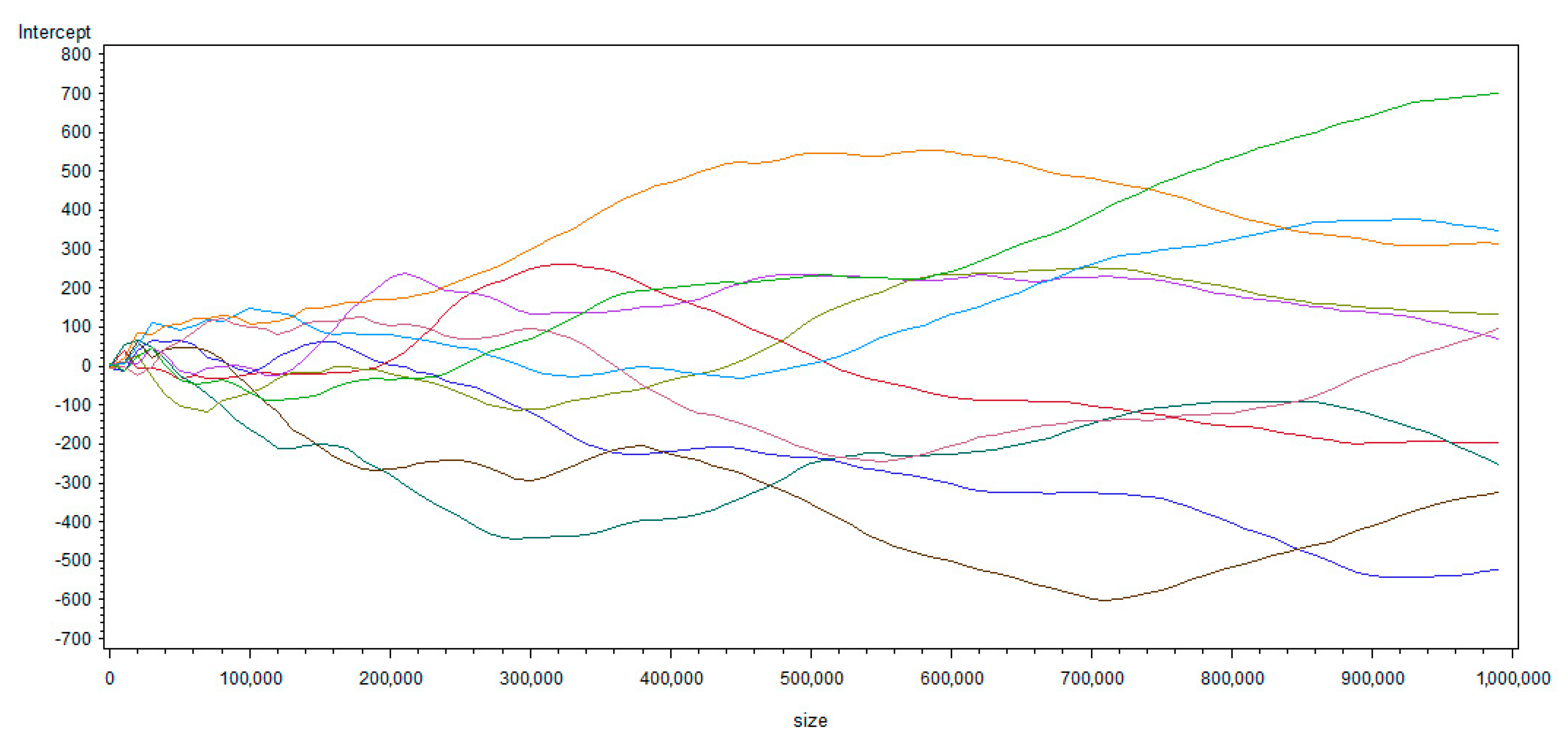
From Figure 3, we observe that, as expected, when $T\to +\infty$, $\widehat{{\beta }_T}$ converges to zero (the magnitude level of $\widehat{{\beta }_T}$ is 10⁻⁵ considering that the decimal precision of the 32-bit computer used is 10⁻⁷, which is almost not-different from zero) and $\widehat{{\alpha }_T}$ is divergent even if the seed values are modified. For 100 different simulations, the conclusions still hold, which indicates that there is no problem of pseudo-randomness in our simulations (even if their conclusions are correct, the simulations by Granger and Newbold (1974) [3] as well as by Nelson and Kang (1981) [11] did not pay attention to the pseudo-randomness, nor specify how the random numbers are obtained). By performing them, as we set all $y_0$ equal to zero, if $\widehat{{\alpha }_T}$ is convergent, then it must converge to $y_0$, in other words, to zero. However, $\widehat{{\alpha }_T}$ seriously deviates from its mathematical expectation zero for different simulations. Thus, the regressions are spurious because the OLS estimator of the trend converges to zero and the other OLS estimator diverges when the sample size tends to infinity.

(3)

From the last column of Table 1, we see that, sometimes, these regressions get a very high R² (the highest being 0.97, with an average of 0.45 for the 100 experiments). This is a classic result associated to spurious regressions, already pointed out by Granger and Newbold (1974) [3].

(4)

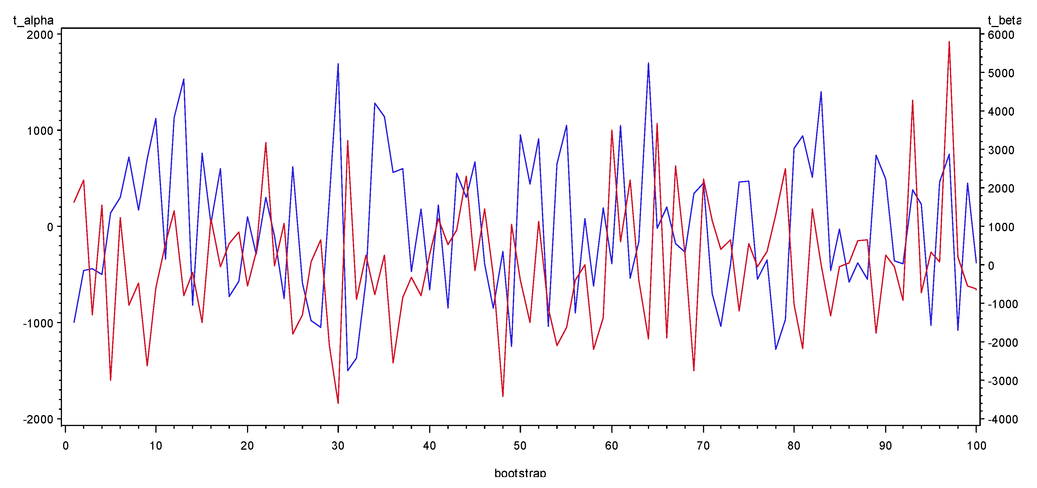
From Table 1 and Figure 4, we see that the t-statistics of the OLS estimators are very high, and that all the p-values of $H_0: \widehat{t_{\widehat{{\alpha }_T}}}=0$ and $H_0: \widehat{t_{\widehat{{\beta }_T}}}=0$ are zero. Thus, the OLS estimators are definitely significant when the sample size tends to infinity. This is also a well-known result associated to spurious regressions, since the residuals are not white noises (as indicated above, and studied by Nelson and Kang (1981) [11], we did not test the correlation of the residuals here). In these conditions, we understand that the usual and fundamental Fisher or Student tests of the OLS estimators are no longer valid, precisely because they are based on the assumption of residuals as white noises. If we use such a detrending method in DS processes, we will indeed get wrong conclusions of significance of the explicative variables.

We understand that our results call for a re-examination of the robustness of the classic findings in macroeconomics. To give an example, in a famous paper, Mankiw, Romer and Weil (1990) [23] identified a significant and positive contribution of education to the per capita GDP growth rate. In a theoretical framework close to a Solowian model, their approach consisted in augmenting a production function with constant returns to scale and decreasing marginal factorial returns, by including a variable of human capital in order to regress, in logarithms, per capita GDP to the investment rates of physical capital and of schooling. Their conclusion is probably accurate; but, as they added a linear trend as a detrending method, whatever the input variable that is selected, it will be found statistically significant as long as the size of their sample is sufficiently large. Our own study has described, in an original manner, the behavior of OLS estimators themselves when the sample size tends to infinity. By comparison, the samples used for simulation by Chan, Hayya and Ord (1977) [10], or Nelson and Kang (1981) [11], are relatively small—even if, obviously, they were extremely useful.

5. Concluding Remarks

The introduction of a linear trend generally aimed at avoiding spurious regressions. However, Nelson and Kang (1981) [11], following Chan, Hayya and Ord (1977) [10], had showed that, in OLS estimates, the assimilation of a difference-stationary process (DS)—the most probable process for GDP, with that of unit root, according to Nelson and Plosser (1982)—to a trend-stationary process (TS), (as did Chow and Li (2002) [24], among others, while the log of China’s GDP may present a unit root) can lead to a situation where the covariance of the residuals depends on the size of the sample, which artificially induces an autocorrelation of the residuals for the lags, and, by generating a pseudo-periodicity in the latter, generates a cyclical movement into the series. However, their analyses mainly focused on the residuals, and their simulated sample size remained small. Here, following Nelson and Kang’s (1981) research line, and using the Chebyshev’s inequality, we have given a strict mathematical proof of the fact that the OLS estimators of a detrending method by adding a linear trend in DS processes are spurious. When the sample size tends to infinity, the OLS estimator of the trend converges toward zero in probability, while the other OLS estimator is divergent. The empirical verification attempted by designing a series through the Monte Carlo method and by performing simulations on a sample of a million observations as an approximation of infinity and true random numbers as seed values has finally provided results consistent with the mathematical proof.

Thus, in the context of what has been specified here, our main conclusion according to which the OLS estimators themselves are spurious when the sample size increases also implies that identifying the nature of time series becomes extremely important. For example, it is crucial to decide whether GDP series are to be treated as TS or DS processes—in a short-run context in which random walks usually look like TS processes (on the basis of many macroeconomic series, Nelson and Plosser (1982) [6] have stated that GDP series would be DS rather than TS processes. More recent studies, such as that by Darné (2009) [25], have reexamined GNP series with new unit root tests, and shown that the US GNP expressed in real terms seems to be a stochastic trend). Even if their effectiveness is questioned, especially because of the sensitivity of the choice of the truncation parameters, we recommend using unit root tests to reduce the risk of inappropriately selecting the detrending method, but by regressing the variables of the models used in the first differences of the logarithm forms when such tests show that they contain unit roots (such an advice has been applied in a recent study on China’s long-run growth using a new time-series database of capital stocks from 1952 to 2014 built through an original methodology. See Long and Herrera (2015, 2016) [26,27]). From a theoretical point of view, regressions in the first differences of the logarithm forms are acceptable both by neoclassic and Keynesian modeling, in which they can easily be interpreted in terms of growth-rate dynamics; and from an econometric point of view, logarithms might be useful when a problem of heteroscedasticity appears, while difference operators can help to avoid spurious regressions if there are unit roots. To avoid the over-differencing problem, we finally recommend using inverse autocorrelation functions (IACFs) to determine the order of integration, along with unit root tests and correlogram (See Cleveland (1972) [28], Chatfield (1979) [29] and Priestey (1981) [30]). That is to say, we suggest the following modeling strategy: (i) if the unit roots tests and correlogram indicate that the variables are stationary in the first differences of the logarithm forms; we stay in traditional time series regressions. (ii) If the variables contain unit roots in the first differences of the logarithm forms, we could pass to cointegration framework or effectuate a second difference operation. (iii) If unit root tests and correlogram both indicate that the series seem be stationary but IACF indicates that the series might be over-differenced (in this case, Autoregressive Function (ACF) and Partial Autoregressive Function (PACF) present characteristics of stationary process (or decrease hyperbolically) while IACF presents characteristics of nonstationary process) that implies an integer order of integration is not sufficient, the true order of integration might be between 0 and 1. That is to say, we might need to pass from traditional time series models to fractal theory (Hosking (1981) [31]) such as AutoRegressive Fractionally Integrated Moving Average (ARFIMA) models or fractional cointegration.

References

1. Wold Herman, O.A. A Study in the Analysis of Stationary Time Series, 2nd ed.; Almqvist and Wiksell: Uppsala, Sweden, 1954. [Google Scholar]
2. Box, G.E.P.; Jenkins, G.M. Time Series Analysis: Forecasting and Control; Holden-Day: San Francisco, CA, USA, 1970. [Google Scholar]
3. Granger, C.W.J.; Newbold, P. Spurious Regressions in Econometrics. J. Econom. 1974, 2, 111–120. [Google Scholar] [CrossRef] [Green Version]
4. Phillips, P.C.B. Understanding Spurious Regressions in Econometrics. J. Econom. 1986, 33, 311–340. [Google Scholar] [CrossRef] [Green Version]
5. Davidson, R.; MacKinnon, J.G. Estimation and Inference in Econometrics; Oxford University Press: New York, NY, USA, 1993. [Google Scholar]
6. Nelson, C.R.; Plosser, C.R. Trends and Random Walks in Macroeconmic Time Series: Some Evidence and Implications. J. Monet. Econ. 1982, 10, 139–162. [Google Scholar] [CrossRef]
7. Engle, R.F.; Granger, C.W.J. Co-integration and Error Correction: Representation, Estimation, and Testing. Econometrica 1987, 55, 251–276. [Google Scholar] [CrossRef]
8. Johansen, S. Estimation and Hypothesis Testing of Cointegration Vectors in Gaussian Vector Autoregressive Models. Econometrica 1991, 59, 1551–1580. [Google Scholar] [CrossRef]
9. Stock, J.H. Asymptotic Properties of Least Squares Estimators of Cointegrating Vectors. Econometrica 1987, 55, 1035–1056. [Google Scholar] [CrossRef]
10. Chan, H.K.; Hayya, J.C.; Ord, J.K. A Note on Trend Removal Methods: The Case of Polynomial Regression Versus Variate Differencing. Econometrica 1977, 45, 737–744. [Google Scholar] [CrossRef]
11. Nelson, C.R.; Kang, H. Spurious Periodicity in Inappropriately Detrended Time Series. Econometrica 1981, 49, 741–751. [Google Scholar] [CrossRef] [Green Version]
12. Rand Corporation. Million Random Digits with 100,000 Normal Deviates; Rand: Santa Monica, CA, USA, 2001. [Google Scholar]
13. Fischer, H. A History of the Central Limit Problem: From Classical to Modern Probability Theory; Sources and Studies in the History of Mathematics and Physical Sciences, Science & Business Media; Springer: Eichstätt, Germany, 2010. [Google Scholar]
14. Knuth, D.E. The Art of Computer Programming: Fundamental Algorithms, 3rd ed.; Addison-Wesley: Boston, CA, USA, 1997. [Google Scholar]
15. Tchebichef, P.L. Des Valeurs moyennes. J. Mathématiques Pures Appliquées 1867, 12, 177–184, (Originally published in 1867 by Mathematicheskii Sbornik, 2, pp. 1–9). [Google Scholar]
16. Box, G.E.P.; Draper, N.R. Empirical Models Building and Response Surfaces; Wiley Series in Probability and Statistics; John Wiley & Sons: New York, NY, USA, 1987. [Google Scholar]
17. Rubinstein, R.Y.; Kroese, D.P. Simulation and the Monte Carlo Method (Vol. 10); John Wiley & Sons: Hoboken, NJ, USA, 2016. [Google Scholar]
18. Creal, D. A survey of sequential Monte Carlo methods for economics and finance. Econom. Rev. 2012, 31, 245–296. [Google Scholar] [CrossRef] [Green Version]
19. Kourtellos, A.; Thanasis, S.; Chih, M.T. Structural threshold regression. Econom. Theory 2016, 32, 827. [Google Scholar] [CrossRef] [Green Version]
20. Lux, T. Estimation of agent-based models using sequential Monte Carlo methods. J. Econ. Dyn. Control 2018, 91, 391–408. [Google Scholar] [CrossRef] [Green Version]
21. Romer, P. The trouble with macroeconomics. Am. Econ. 2016, 20, 1–20. [Google Scholar]
22. Reed, W.R.; Zhu, M. On estimating long-run effects in models with lagged dependent variables. Econ. Model. 2017, 64, 302–311. [Google Scholar] [CrossRef]
23. Mankiw, N.G.; Romer, D.; Weil, D.N. A Contribution to the Empirics of Economic Growth. Q. J. Econ. 1992, 107, 407–427. [Google Scholar] [CrossRef]
24. Chow, G.C.; Li, K.W. China’s Economic Growth: 1952–2010. Econ. Dev. Cult. Chang. 2002, 51, 247–256. [Google Scholar] [CrossRef]
25. Darné, O. The Uncertain Unit Root in Real GNP: A Re-Examination. J. Macroecon. 2009, 31, 153–166. [Google Scholar] [CrossRef]
26. Long, Z.; Herrera, R. A Contribution to Explaining Economic Growth in China: New Time Series and Econometric Tests of Various Models; Mimeo, CNRS UMR 8174—Centre d’Économie de la Sorbonne: Paris, France, 2015. [Google Scholar]
27. Long, Z.; Herrera, R. Building Original Series of Physical Capital Stocks for China’s Economy: Methodological Problems, Proposals of Solutions and a New Database. China Econ. Rev. 2016, 40, 33–53. [Google Scholar] [CrossRef]
28. Cleveland, W.S. The Inverse Autocorrelations of a Time Series and Their Applications. Technometrics 1972, 14, 277–298. [Google Scholar] [CrossRef]
29. Chatfield, C. Inverse Autocorrelations. J. R. Stat. Soc. 1979, 142, 363–377. [Google Scholar] [CrossRef]
30. Priestley, M.B. Spectral Analysis and Time Series, 1: Univariate Series; Probability and Mathematical Statistics; Academic Press: London, UK, 1981. [Google Scholar]
31. Hosking, J.R.M. Fractional differencing. Biometrika 1981, 68, 165–176. [Google Scholar] [CrossRef]
Figure 1. Evolutions of α T ^ when the sample size increases from 100 up to 1,000,000.
Mathematics 08 01931 g001
Figure 2. Evolutions of β T ^ when the sample size increases from 100 up to 1,000,000.
Mathematics 08 01931 g002
Figure 3. Simulations of α T ^ (in red) and β T ^ (in blue).
Mathematics 08 01931 g003
Figure 4. Simulations of t α T ^ ^ (in red) and t β T ^ ^ (in blue).
Mathematics 08 01931 g004