Constrained Mixed-Variable Design Optimization Based on Particle Swarm Optimizer with a Diversity Classifier for Cyclically Neighboring Subpopulations

Abstract

In this research, an easy-to-use particle swarm optimizer (PSO) for solving constrained engineering design problems involving mixed-integer-discrete-continuous (MIDC) variables that adopt two kinds of diversity-enhancing mechanisms to achieve superior reliability and validity was developed. As an initial diversity-boosting tool, the local neighborhood topology of each particle is set up such that information exchange is restricted to a limited number of consecutively numbered particles. This topological mechanism forces each particle to move in the search space while interacting only with its neighboring subpopulation. The second diversity-enhancing task is to ensure that the exploration behavior of each particle in the search space is governed such that it follows the diversity classifier decision applied to its subpopulation. This diversity classification iteratively adjusts the three-phase velocity-related mechanism of each particle such that it approaches or retreats from its previous best position/the current best position among the subpopulation. In summary, this PSO tool not only introduces the social interaction of the particle within its cyclically neighboring subpopulation but also exploits the three-phase velocity behavior law governed by the distributed diversity measures categorized for each neighboring subpopulation. This scheme has superior reliability, as well as high practicality for engineering optimization problems involving MIDC variables, which are handled by the widely adopted straightforward rounding-off technique used in most swarm-inspired metaheuristic search technologies.

1. Introduction

Several real-life engineering design tasks require the use of numerical optimization techniques that can handle highly nonlinear multimodal problems, with several complicated constraints on factors such as stress, deflection, load-carrying capability, and geometric configuration [1]. Although several gradient-based deterministic algorithms have been introduced during the past decades, their solution is a function of the initial search points and thus might not be the global optimum. This drawback of classical methods has induced the widespread adoption of biologically inspired metaheuristic algorithms; i.e., algorithms that mimic the behavior of different species or the social-cooperative behavior of swarms [1,2,3]. Some popular metaheuristic optimizers include the differential evolution (DE) algorithm, genetic algorithm (GA), particle swarm optimization (PSO), simulated annealing (SA) algorithm, and ant colony optimization. In this area of research, the PSO algorithm has attracted much attention as a reliable treatment for a wide range of large-scale, multimodal, non-convex, and nonlinear unconstrained optimization problems [4,5].

When handling engineering optimization problems via PSO, one frequently faces the following two obstacles.

(I)

Most engineering design tasks include multiple real-life physical constraints and thus necessitate PSO techniques that can account for these. Furthermore, such physical constraints are, in general, treated as hard constraints that should be satisfied by any feasible solution found via the optimization procedure.

(II)

A large fraction of design problems in engineering fields belong in the category of mixed-integer-discrete-continuous (MIDC) optimization problems and thus particular care has to be taken to find feasible solutions, which makes design tasks more challenging.

However, since PSO was initially devised not only to handle unconstrained optimization problems but also to work only with real-valued variables, the presence of non-continuous design variables results increases the difficulty of finding feasible or optimal solutions, as in most other evolutionary algorithms [6,7,8,9,10]. Trends and ways of tackling constrained mixed-variable problems in evolutionary algorithms can be found in several articles [9,11,12,13,14,15,16,17,18,19,20,21]. Nevertheless, a rigorous mechanism for handling integer/discrete variables is still challenging and the focus of intensive research, even in PSO applications for unconstrained optimization problems, as mentioned in [6].

Recently, [10] preliminarily investigated a straightforward procedure for solving constrained MIDC optimal design problems. In their research, they recommended a constrained PSO algorithm combined with the conventional technique of rounding the variable values to the nearest discrete or integer values for objective function evaluation, while all particles still freely evolve with floating-point values within a continuous search domain, regardless of the type of variable. Although this primitive technique seems to be rather unrefined, it has been widely introduced with promising application results in several studies on evolutionary algorithms [11,12,13,14,15,16,17,18,19,20,21]. Nevertheless, their constrained PSO-based method combined with the rounding-off mechanism may not guarantee acceptable reliability; i.e., the probability of finding the required design variables satisfying the optimality criteria may be insufficient. This performance degradation is certainly due to the insufficient diversification characteristics of swarms, which, in practical implementation, may accelerate the premature convergence phenomenon of particles to a local optimum. It should be noted that diversification helps the optimizer to explore the search space on a global scale, possibly resulting in the exploration of various diverse solutions for attaining global optimality [1]. However, most population-based evolutionary computation techniques, including PSO, depend on the basic underlying principle of reducing the search space in the progression toward a global optimum. Updating the position vector for each particle that outperforms the current global best position of the population could no longer be achieved after a certain iteration number owing to the swarm-movement pattern and, in this case, the whole swarm may remain trapped in a search region containing a local optimal solution [22,23]. In such a case, if a method to enhance population diversity is not introduced, particles evolving based on the conventional PSO mechanism may have difficulty reaching the true global optimal position. Such a diversity improvement is expected to motivate research studies of our diversity-guided PSO with a cyclic network mechanism.

The purpose of the present study is the realization of an easy-to-use diversity-guided PSO scheme for constrained mixed-variable optimization problems, which uses diversity classifiers for cyclically neighboring subpopulations and is characterized by superior reliability and validity. To achieve this aim, this paper develops a novel constrained PSO strategy that combines the following two kinds of diversity-enhancing mechanisms. The first diversity-boosting tool is to construct cyclically neighboring multi-subpopulations, one for each particle (host particle), where the subpopulation is composed of some successively numbered particles, with the host particles as the center. In this structure, the host particle only interacts with a limited number of neighboring particles (i.e., particles belonging to the subpopulation) during the search process within the problem-solution space. Thus, the “nearby neighbor” in this mechanism implies the particle within the subpopulation that transfers individual positional information and fitness values to the host particle [24,25,26]. Note that the host particle of a certain subpopulation can be one of several nearby neighbors of other subpopulations; thus, any information on the good fitness value of one host particle is cyclically propagated to other neighboring host particles during the evolution process. Therefore, this structure forces each particle to achieve social learning from its respective neighborhoods and not directly from the best position of the entire swarm, which results in enhancing the population diversity. Second, to achieve diversity improvement for each subpopulation, the aforementioned PSO mechanism is extended and combined with the three-phase velocity update law, which is introduced to governs the behavior of the host particles at each iteration. In this extended PSO algorithm, the velocity behavior of each host particle per iteration is governed by attraction, repulsion, and in-between phases [23,27], chosen according to the diversity classifier applied to the subpopulation of the host particle. In summary, our PSO scheme not only exploits constricted social learning of each particle through cyclically neighboring subpopulations but also incorporates the three-phase velocity behavior law, implemented by following the locally distributed diversity measures categorized for each subpopulation. This novel PSO scheme features high reliability, as well as superior practicality for engineering optimization problems involving MIDC variables, which are handled via the straightforward rounding-off technique that has been widely adopted in swarm-inspired metaheuristic search technologies. Note that the conventional PSO scheme proposed by [23,27] evaluates the sole diversity measure obtained from the position data of the entire swarm and targets optimization problems having continuous variables and no constraint functions. Therefore, their method may not reliably provide a sufficient level of population diversity to produce offspring that outperform their parents, in the case of MIDC nonlinear programming with multimodal characteristics; even when no constraint is involved. Several benchmark MIDC design problems are presented to clearly verify that the proposed PSO scheme is a highly useful tool, providing remarkable reliability.

The remainder of this paper is organized as follows. In the following section, typical MIDC engineering design problems and a brief sketch of the conventional evolutionary PSO algorithm are presented. In Section 3, the development of a novel PSO scheme with a diversity classifier for cyclically neighboring subpopulations is described, and its distinctive features are discussed in depth. The details of eight typical benchmark design examples are given in the successive sections, and then, simulation results obtained using the proposed PSO tool are compared in depth with those obtained using other PSO methods and various other evolutionary algorithms. Further discussions on the influence of variations in neighboring particle sizes on the performance of the proposed PSO scheme are also presented. Finally, we present our conclusions in Section 5.

2. Engineering Design Problem and Particle Swarm Optimizer

The classical PSO is a population-based stochastic computational technique with a powerful global search capability for resolving the following form of the optimization problem, without constraints:

$$\begin{array}{c}\hfill minf\left(\mathit{x}\right),\mathrm{over}\mathit{x}\in {\mathbb{R}}^n\mathrm{and}f\left(\mathit{x}\right):{\mathbb{R}}^n\mapsto \mathbb{R}\end{array}$$

(1)

where the linear or nonlinear objective function $f:{\mathbb{R}}^n\mapsto \mathbb{R}$ is minimized with respect to the vector of design variables $\mathit{x}\in {\mathbb{R}}^n$. Therefore, a particle in the PSO algorithm represents a potential solution $\mathit{x}$ in (1). Let $\mathbb{D}$ denote the limited sub-region of an entire n-dimensional Euclidean space and be assumed to contain the optimal solutions. The conventional evolutionary PSO searching mechanism is initiated with a swarm randomly generated over the space $\mathbb{D}$. Thereafter, each particle moves in a coordinated way through the n-dimensional search space $\mathbb{D}$. The behavior of each particle is mainly influenced by both its own best previous experience and a social compulsion to move toward a single best particle among the entire swarm, as follows:

$$\begin{array}{cc}\hfill {\mathit{x}}_i^{k+1}& ={\mathit{x}}_i^k+{\mathit{v}}_i^{k+1},\hfill \end{array}$$

(2)

$$\begin{array}{cc}\hfill {\mathit{v}}_i^{k+1}& =c_0{\mathit{v}}_i^k+c_1{r}_{1,i}^k({\mathit{x}}_{\mathrm{pbest},i}-{\mathit{x}}_i^k)+c_2{r}_{2,i}^k({\mathit{x}}_{\mathrm{gbest}}-{\mathit{x}}_i^k)\hfill \end{array}$$

(3)

where $i=1,2,\cdots ,n_p$ denotes the index of the particle where $n_p$ is the number of particles in the swarm; $k=1,2,\cdots ,k_{\max }$ represents the iteration number where $k_{max}$ is the maximum number of allowable iterations; ${\mathit{x}}_i^k\in {\mathbb{R}}^n$ and ${\mathit{v}}_i^k\in {\mathbb{R}}^n$ denotes the position and velocity vectors, respectively, for the ith particle at the k-th iteration; ${\mathit{x}}_{\mathrm{pbest},i}$ denotes the vector of the best previous position yielding the minimum fitness value $f(·)$ for the ith particle; ${\mathit{x}}_{\mathrm{gbest}}$ denotes the vector of the global best position found by the entire swarm; $c_0$ denotes the inertia weight and $c_1$ and $c_2$ represent the cognitive and social scaling parameters, respectively; and $r_{1,i}^k$ and $r_{2,i}^k$ are random parameters generated uniformly in the range of $[0,1]$.

However, the above classical PSO method frequently faces the following two obstacles. First, for engineering optimal design problems that include several physical constraints, it necessarily introduces a technique that is capable of handling the problem (1), subject to

$$\mathbb{F}:=\{\mathit{x}\in {\mathbb{R}}^n|h_1\left(\mathit{x}\right)\le 0,h_2\left(\mathit{x}\right)\le 0,h_3\left(\mathit{x}\right)\le 0,\cdots ,h_m\left(\mathit{x}\right)\le 0\},$$

(4)

where $h_{\ell }\left(\mathit{x}\right):{\mathbb{R}}^n\mapsto \mathbb{R}$ denotes the constraint function and a feasible region denoted by $\mathbb{F}$ represents the set of design variables that satisfy the given constraint conditions. It should be noted that $h_{\ell }\left(\mathit{x}\right)\le 0$, $\ell =1,2,\cdots ,m$ in (4) is generally treated as a hard constraint in most engineering design problems. It is therefore critical to handle such constraint functions within the framework of PSO for evaluating the fitness of each particle over the PSO iteration and eventually obtaining the resultant optimal vector ${\mathit{x}}^{*}$. Second, in practical engineering design work, some or all optimization problem design variables very commonly have integer/discrete values, as

$$\mathit{x}:={({\mathit{x}}^{\mathrm{I}},{\mathit{x}}^{\mathrm{D}},{\mathit{x}}^{\mathrm{C}})}^T={(x_1^{\mathrm{I}},x_2^{\mathrm{I}},\cdots ,x_{n_{\mathrm{I}}}^{\mathrm{I}},x_1^{\mathrm{D}},x_2^{\mathrm{D}},\cdots ,x_{n_{\mathrm{D}}}^{\mathrm{D}},x_1^{\mathrm{C}},x_2^{\mathrm{C}},\cdots ,x_{n_{\mathrm{C}}}^{\mathrm{C}})}^T$$

(5)

where the number of design variables becomes $n:=n_{\mathrm{I}}+n_{\mathrm{D}}+n_{\mathrm{C}}$. Let the feasible subsets of integers and discrete and continuous design variables, be denoted by ${\mathbb{R}}^{n_{\mathrm{I}}}$, ${\mathbb{R}}^{n_{\mathrm{D}}}$ and ${\mathbb{R}}^{n_{\mathrm{C}}}$. Using this information, researchers have tried to modify the original PSO scheme to handle constraint conditions, as well as integers and discrete variables [6,7,8,9,10,11,12,13,14,15,16,17,18,19,20,21]. In the following section, we propose an easy-to-use PSO scheme with a diversity classifier for cyclically neighboring subpopulations, which allows superior reliability and validity for constrained MIDC optimization problems.

3. PSO with a Diversity Classifier for Cyclically Neighboring Subpopulations

To improve the behavior performance of the swarm via a diversity-boosting mechanism, [23,27] studied a diversity-guided PSO (ATRE-PSO) strategy. Comparing to (3), the sole velocity update law for each particle is modified so that its velocity behavior follows one of the three-phase update laws, where the attraction, in-between, and repulsion phases are classified by the diversity measure $\mathrm{DIV}(·)$ per iteration, as follows:

$${\mathit{v}}_i^{k+1}=\left\{\begin{array}{cc}{c}_0{\mathit{v}}_i^k+c_1{r}_{1,i}^k({\mathit{x}}_{\mathrm{pbest},i}-{\mathit{x}}_i^k)+c_2{r}_{2,i}^k({\mathit{x}}_{\mathrm{gbest}}-{\mathit{x}}_i^k)\hfill & \mathrm{if}\mathrm{DIV}\left(k\right)>{\mathrm{D}}_{\mathrm{high}};\hfill \\ c_0{\mathit{v}}_i^k-c_1{r}_{1,i}^k({\mathit{x}}_{\mathrm{pbest},i}-{\mathit{x}}_i^k)-c_2{r}_{2,i}^k({\mathit{x}}_{\mathrm{gbest}}-{\mathit{x}}_i^k)\hfill & \mathrm{if}\mathrm{DIV}\left(k\right)<{\mathrm{D}}_{\mathrm{low}};\hfill \\ c_0{\mathit{v}}_i^k+c_1{r}_{1,i}^k({\mathit{x}}_{\mathrm{pbest},i}-{\mathit{x}}_i^k)-c_2{r}_{2,i}^k({\mathit{x}}_{\mathrm{gbest}}-{\mathit{x}}_i^k)\hfill & \mathrm{otherwise},\hfill \end{array}\right.$$

(6)

where ${\mathrm{D}}_{\mathrm{high}}$ and ${\mathrm{D}}_{\mathrm{low}}$ are chosen by the designer. The diversity classifier for each iteration is obtained by

$$\begin{array}{c}\hfill \mathrm{DIV}\left(k\right)=\frac{1}{n_p}\sum _{i=1}^{n_p}\sqrt{\sum _{j=1}^n{\left({\mathit{x}}_{i,j}^k-{\widehat{\mathit{x}}}_j^k\right)}^2},{\widehat{\mathit{x}}}_j^k:=\frac{1}{n_p}\left(\sum _{\ell =1}^{n_p}{\mathit{x}}_{\ell ,j}^k\right).\end{array}$$

(7)

where ${\mathit{x}}_{i,j}$ denotes the jth entry of ${\mathit{x}}_i$. They verified that their diversity-boosting mechanism allows particles to maintain an acceptable level of diversity for various benchmark problems with continuous variables and no constraint functions and thus helps to address the premature convergence problem. However, the above method may not reliably provide a level of population diversity that is sufficiently high to produce offspring that outperform their parents in the case of MIDC nonlinear programming with multimodal characteristics, even when no constraint is involved. Therefore, the PSO scheme that exploits the constricted social learning of each particle through cyclically neighboring subpopulations is presented in the following and such a scheme is extended for combination with the three-phase velocity update law to achieve diversity improvement for each subpopulation.

To consider the constraint functions of the optimization problem within the framework of our PSO algorithm, an efficient constraint handling mechanism introducing a so-called virtual objective function, $f_v\left(\mathit{x}\right):{\mathbb{R}}^n\mapsto \mathbb{R}$, is summarized below [28]. Note that any function can be such a virtual objective function if it guarantees that: (i) for any $\mathit{x}\in {\mathbb{R}}^n$ satisfying all constraint conditions, $f_v\left(\mathit{x}\right)<0$ holds; and (ii) for any ${\mathit{x}}_i\in {\mathbb{R}}^n$ and ${\mathit{x}}_j\in {\mathbb{R}}^n$, satisfying $f\left({\mathit{x}}_i\right)<f\left({\mathit{x}}_j\right)$, $f_v\left({\mathit{x}}_i\right)<f_v\left({\mathit{x}}_j\right)$ holds. For example, the function $\arctan \left\{f\right(\mathit{x}\left)\right\}-\pi /2$ can be a virtual function satisfying the above two properties (refer to [10,28] for details). Then, the given optimization problem (1) subject to (4) can be transformed into the following unconstrained optimization problem:

$$\underset{\mathit{x}\in {\mathbb{R}}^n}{min}\mathcal{L}\left(\mathit{x}\right),\mathcal{L}\left(\mathit{x}\right):=\left\{\begin{array}{cc}{h}_{max}\left(\mathit{x}\right),\hfill & \mathrm{if}{h}_{max}\left(\mathit{x}\right)\ge 0;\hfill \\ f_v\left(\mathit{x}\right),\hfill & \mathrm{otherwise},\hfill \end{array}\right.$$

(8)

where $h_{max}\left(\mathit{x}\right)$ is defined as $h_{max}\left(\mathit{x}\right):=max\left(h_1\left(\mathit{x}\right),h_2\left(\mathit{x}\right),\cdots ,h_m\left(\mathit{x}\right)\right)$. This modified objective function forces the swarm to keep moving into and remaining within the bounds of feasible space $\mathbb{F}$ during the initial iteration steps and then moving through the solution space to search for the optimum. Therefore, this constraint handling strategy enables one to obtain feasible design variables that, at least, satisfy the constraint conditions in a considerably more simple manner.

Next, to solve the unconstrained problem (8), the PSO scheme exploiting the constricted social learning of each particle through cyclically neighboring subpopulations is extended to incorporate the three-phase velocity behavior law (2) implemented by following the locally distributed diversity measures categorized for each subpopulation. In the canonical PSO strategy, the offspring of each particle is produced based on the information on its best previous position vector ${\mathit{x}}_{\mathrm{pbest},i}$ and the information on the current swarm best position vector ${\mathit{x}}_{\mathrm{gbest}}$, as shown in (3). This means that because ${\mathit{x}}_{\mathrm{gbest}}:=arg{min}_{\mathit{x}\in \left\{{\mathit{x}}_{\mathrm{pbest},i}\right|i=1,\cdots ,n_p\}}\mathcal{L}\left(\mathit{x}\right)$, (i.e., ${\mathit{x}}_{\mathrm{gbest}}$ is determined from all ${\mathit{x}}_{\mathrm{pbest},i}$ available at each evolutionary stage), ${\mathit{x}}_{\mathrm{pbest},i}$ may be mainly responsible for premature convergence [29]. Considering this viewpoint, the swarm flexibility is boosted by constructing cyclically neighboring multi-subpopulations, one for each particle (host particle), which results in the replacement of only one ${\mathit{x}}_{\mathrm{gbest}}$ by different social-best positions for each subpopulation. Such a social-best position vector for the i-th particle ${\mathit{x}}_i$ at the k-th iteration, denoted by ${\mathit{x}}_{\mathrm{sbest},i}^k$, is determined only from its individual subpopulation, as follows:

$${\mathit{x}}_{\mathrm{sbest},i}^k:=arg\underset{\mathit{x}\in \left\{{\mathit{x}}_{\ell }^k\right|\ell =i-\frac{n_s}{2},\cdots ,i+\frac{n_s}{2}\}}{min}\mathcal{L}\left(\mathit{x}\right)$$

(9)

where an even number of $n_s(\le n_p)$ denotes the total number of neighboring particles within the subpopulation of ${\mathit{x}}_i$, and ${\mathit{x}}_{\ell }^k:={\mathit{x}}_{(\ell -1\mathrm{mod}{n}_p)+1}^k$ for $\ell <1$ or $n_p+1\le \ell$. This formulation verifies that the host particle ${\mathit{x}}_i$ interacts only with a limited number of particles belonging to the same subpopulation and those nearby neighbor particles transfer their positional information and fitness values to the host particle. Furthermore, the host particle of a certain subpopulation can be a nearby neighbor of some other subpopulation, which means that any information on the good fitness value of one host particle is cyclically propagated to other neighboring host particles during the evolution process. Therefore, this structure forces each particle to achieve social learning from its respective neighborhoods, not directly from the best position of the entire swarm, resulting in the enhancement of population diversity. It then follows that by replacing ${\mathit{x}}_{\mathrm{gbest}}$ in (6) with ${\mathit{x}}_{\mathrm{sbest},i}^k$ in (9) that

$${\mathit{v}}_i^{k+1}=c_0{\mathit{v}}_i^k\pm c_1{r}_{1,i}^k({\mathit{x}}_{\mathrm{pbest},i}-{\mathit{x}}_i^k)\pm c_2{r}_{2,i}^k({\mathit{x}}_{\mathrm{sbest},i}^k-{\mathit{x}}_i^k)$$

(10)

where the positive and negative signs are assigned according to the diversity measure $\mathrm{DIV}\left(k\right)$ at each iteration. This formulation implies that ${\mathit{v}}_i^k$ enforces the accelerated movement of ${\mathit{v}}_i^k$ toward ${\mathit{x}}_{\mathrm{pbest},i}$ and ${\mathit{x}}_{\mathrm{sbest},i}^k$. Conversely, the existing PSO method proposed by [23,27] governs the swarm behavior of all particles by following the sole diversity measure, $\mathrm{DIV}\left(k\right)$ in (7), derived from the position data of the entire population. Therefore, such a diversity classifier mechanism should be modified to be compatible with the swarm structure of cyclically neighboring multi-subpopulations. This can be achieved by developing multiple distributed diversity measures categorized for each local subpopulation as follows: for $i=1,2,\cdots ,n_p$,

$$\begin{array}{c}\hfill {\mathrm{DIV}}_i\left(k\right)=\frac{1}{n_s+1}\sum _{\ell =i-\frac{n_s}{2}}^{i+\frac{n_s}{2}}\sqrt{\sum _{j=1}^n{\left({\mathit{x}}_{\ell ,j}^k-{\widehat{\mathit{x}}}_j^k\right)}^2},{\widehat{\mathit{x}}}_j^k:=\frac{1}{n_s+1}\left(\sum _{l=i-\frac{n_s}{2}}^{i+\frac{n_s}{2}}{\mathit{x}}_{l,j}^k\right),\end{array}$$

(11)

where ${\mathrm{DIV}}_i\left(k\right)$ refers to the diversity measure of ${\mathit{x}}_i^k$ updated in each iteration. For $n_p=9$ and $n_s=4$, the overall schematic diagram of our PSO with diversity classifiers applied respectively to cyclically neighboring multi-subpopulations is illustrated in Figure 1. In this figure, the first particle has ${\mathrm{DIV}}_1\left(k\right)>{\mathrm{D}}_{\mathrm{high}}$ and thus moves toward both pbest and sbest. In contrast, since ${\mathrm{DIV}}_2\left(k\right)<{\mathrm{D}}_{\mathrm{low}}$, the second particle moves in the direction opposite to that of pbest and sbest. The ninth particle with ${\mathrm{D}}_{\mathrm{low}}\le {\mathrm{DIV}}_9\left(k\right)\le {\mathrm{D}}_{\mathrm{high}}$ moves toward pbest but in the direction opposite to that of sbest.

Finally, a straightforward and reliable method for handling the MIDC design variables in (5) by applying the aforementioned PSO strategy in (2) and (10) with (11) is described. To achieve this objective, we introduce the widely used rounding-off technique, as follows.

(I)

Initialize the entire swarm. Then, the particles evolve in the $\mathbb{D}$-dimensional search space, regardless of the variable types in ${\mathit{x}}_i(:={({\mathit{x}}^{\mathrm{I}},{\mathit{x}}^{\mathrm{D}},{\mathit{x}}^{\mathrm{C}})}^T)$, of (5), via (2) and (10) with ${\mathit{x}}_{\mathrm{sbest},i}^k$. As a result, all elements (i.e., all design variables) in ${\mathit{x}}_i$ take floating-point values during the current stage.

(II)

For $j=1,2,\cdots ,n_{\mathrm{I}}$, the variable $x_{i,j}$, which is the jth entry of ${\mathit{x}}_i\in \mathbb{R}$, denotes the integer design variable $x_{i,j}^{\mathrm{I}}$ and thus must take an integer value. Let $\mathrm{INT}\left(x_{i,j}\right)$ denote the nearest integer of $x_{i,j}\in \mathbb{R}$. i.e., $x_{i,j}$ is rounded to its nearest integer. It then follows that $x_{i,j}^{\mathrm{I}}\leftarrow \mathrm{INT}\left(x_{i,j}\right)$ is performed. Similarly, the discrete design variable $x_{i,n_{\mathrm{I}}+\ell }^{\mathrm{D}}$ for $\ell =1,2,\cdots ,n_{\mathrm{D}}$ takes the value of $\mathrm{DIS}\left(x_{i,n_{\mathrm{I}}+\ell }\right)$ as $x_{i,n_{\mathrm{I}}+\ell }^{\mathrm{D}}\leftarrow \mathrm{DIS}\left(x_{i,n_{\mathrm{I}}+\ell }\right)$. Here, $\mathrm{DIS}\left(x_{i,n_{\mathrm{I}}+\ell }\right)$ indicates the nearest discrete value that $x_{i,n_{\mathrm{I}}+\ell }$ takes in the given data set of discrete design values.

(III)

Fitness of individual particle with positional vector $({\mathit{x}}_i^{\mathrm{I}},{\mathit{x}}_i^{\mathrm{D}},{\mathit{x}}_i^{\mathrm{C}})$, is evaluated based on the objective function $\mathcal{L}\left(\mathit{x}\right)$, as in (8) subject to no constraint functions. Finally, ${\mathit{x}}_{\mathrm{pbest},i}$ and ${\mathit{x}}_{\mathrm{sbest},i}^k$ in (9), are calculated.

For finding an optimal design variable vector, the aforementioned procedure for a set of $n_p$ particles keeps running until a certain termination criterion is met. Then, after a significant number of evolutions, optimal variables or approximate optimal variables are expected to be found. For handling constrained optimization problems with the MIDC variables, the flowchart of the overall PSO with a diversity classifier for cyclically neighboring subpopulations is illustrated in Figure 2, where the optimal design variable vector ${\mathit{x}}^{*}$ is determined as

$${\mathit{x}}^{*}:=arg\underset{\mathit{x}\in \left\{{\mathit{x}}_i^j\right|i=1,2,\cdots ,n_p;j=1,2,\cdots ,k\}}{min}\mathcal{L}\left(\mathit{x}\right).$$

(12)

Conversely, the presented flowchart includes an optional mechanism such that, after a predetermined number of evolutions, $k_{\mathrm{DIV}}$, the velocity-related behavior of the particle is governed by the formula of (3), with ${\mathit{x}}_{\mathrm{sbest},i}^k$ instead of ${\mathit{x}}_{\mathrm{gbest}}$. This mechanism only emphasizes the fine-searching ability via an attraction phase among particles belonging to the same subpopulation in the current search space that is sufficiently narrowed via the movement of the particles over the previous evolutions with the three-phase velocity update law.

4. Numerical Experimentation

This section introduces a wide variety of benchmark design problems that involve different types of MIDC variables and are subject to real-life design constraints for evaluating the performance of the proposed optimization algorithm. The 30 independent runs of the optimization task for each design problem were executed, where the user parameters were set as $c_0=0.7298$ and $c_1=c_2=1.4962$. The maximum PSO iteration number was set as $k_{max}=1500$, for the car side impact design problem, and $k_{max}=500$ for the others. The swarm size was $n_p=50$ for the design problem of the reinforced concrete beam and $n_p=100$ for the others. To verify the practicality and reliability of the proposed PSO-based design method, the statistical results were primarily compared with several existing heuristic techniques [1,2,3,30], in which the authors extensively survey several evolutionary- and nature-inspired algorithms. Conversely, the relation between the neighborhood size, $n_s$, and the robustness and preciseness of the PSO algorithm is studied in-depth, and one possible promising indicator for determining $n_s$ is then discussed.

4.1. Optimal Design of Pressure Vessel

The design problem for a compressed air storage tank in Figure 3, where the cylindrical pressure vessels are capped at both ends by two hemispherical heads, is examined. Its minimum volume is 750 (${\mathrm{f}\mathrm{t}}^3$), and the working pressure is 3000 (psi). The design objective is to minimize the total manufacturing cost, which comprises a combination of material, forming, and welding costs. Four kinds of design variables are defined as (1) the inner radius of the shell, r; (2) the length of the cylindrical section, l; (3) the thickness of the head, $t_h$; (4) the thickness of the shell, $t_s$. Let $\mathit{x}:={(x_1,x_2,x_3,x_4)}^T$ be defined as $\mathit{x}={(l,r,t_s,t_h)}^T$. Here, l and r are continuous variables but the available thicknesses for $t_h$ and $t_s$ are integer multiples of $0.0625$. Then, the optimal design problem is formulated as

$$\begin{array}{c}\hfill \underset{\mathit{x}}{min}f\left(\mathit{x}\right):=0.6224x_3{x}_2{x}_1+1.7781x_4{x}_2^2+3.1661x_3^2{x}_1+19.84x_3^2{x}_2\end{array}$$

(13)

subject to the constraint conditions, which are in accordance with the ASME design codes, such as

$$\begin{array}{cc}\hfill & h_1\left(\mathit{x}\right):=0.0193x_2-x_3\le 0\hfill \end{array}$$

(14)

$$\begin{array}{cc}\hfill & h_2\left(\mathit{x}\right):=0.00954x_2-x_4\le 0\hfill \end{array}$$

(15)

$$\begin{array}{cc}\hfill & h_3\left(\mathit{x}\right):=750\times 1728-\pi x_2^2{x}_1-\frac{4}{3}\pi x_2^3\le 0,,\hfill \end{array}$$

(16)

$$\begin{array}{cc}\hfill & h_4\left(\mathit{x}\right):=x_1-240\le 0,\hfill \end{array}$$

(17)

where $h_3\left(\mathit{x}\right)$ denotes the constraint function concerning the minimum volume of 750 (${ft}^3$). The lower bound of the design variable $x_1$ is fixed at 20 (in) whereas its upper bound is set at 240 (in), accounting for the constraint $h_4\left(\mathit{x}\right)$. Note that this differs from the limit of 200 (in), as described in some articles [1,2]. When the limit of $x_1$ has been determined, the ranges of $x_2$, $x_3$, and $x_4$ are automatically derived through the constraint conditions as: $x_2\in [37.7,63]$, $x_3\in [0.6875,1.25]$, and $x_4\in [0.3125,0.625]$.

The optimizing procedure presented in Figure 2 is executed to find the optimal decision variable vector ${\mathit{x}}^{*}$ that achieves the minimum cost function $f\left(\mathit{x}\right)$ and simultaneously satisfies the four constraints on $h_i\left(\mathit{x}\right)$. The modified unconstrained problem (8) is defined with $f_v\left(\mathit{x}\right):=\arctan \left\{f\left(\mathit{x}\right)\right\}-\pi /2$, and $({\mathrm{D}}_{\mathrm{low}},{\mathrm{D}}_{\mathrm{high}},k_{\mathrm{DIV}})=(10,20,150)$. The best solution and corresponding optimal objective function value are compared with several evolutionary and nature-inspired algorithms in

Table 1. Optimization results for the pressure vessel design problem.

Method	[32] PSO-GA	[31] HS	[33] SA-DS	[1] FA	[2] PSO	Present Study PSO (${\mathit{n}}_{\mathit{s}}\mathbf{=}\mathbf{16}$)
$x_1$ (l)	221.365487	221.36553	207.22555	221.36547	221.365548	221.3654714
$x_2$ (r)	38.860102	38.86010	39.80962	38.86010	38.860099	38.8601036
$x_3$ ($t_s$)	0.7500	0.75	0.7683	0.75	0.75000	0.7500000
$x_4$ ($t_h$)	0.3750	0.375	0.3797	0.375	0.37500	0.3750000
$h_1\left({\mathit{x}}^{*}\right)$	−0.0000	−0.0000	−0.0000	−0.0000	−0.000000	−0.0000000
$h_2\left({\mathit{x}}^{*}\right)$	−0.0043	−0.0043	−0.0000	−0.0043	−0.004275	−0.0042746
$h_3\left({\mathit{x}}^{*}\right)$	0.0446	0.2713	−10.7065	−0.0134	−0.000190	−0.0255540
$h_4\left({\mathit{x}}^{*}\right)$	−18.6345	−18.6345	−32.7744	−18.6345	−18.634452	−18.6345290
Best objective value	5850.383064	5849.76169	5868.76484	5850.38306	5850.38376	5850.38306
Objective deviation a	$1.0+6.837\times {10}^{-10}$	$1.0-1.062\times {10}^{-4}$	$1.0+3.142\times {10}^{-3}$	1.0	$1.0+1.197\times {10}^{-7}$	1.0
Feasibility	Infeasible	Infeasible	Feasible	Feasible	Feasible	Feasible
Worst objective value	N/A b	N/A	6804.328100	6258.96825	5850.591797	5850.38308
Average objective value	N/A	N/A	6164. 585867	5937.33790	N/A	5850.38306
Standard deviation	N/A	N/A	257.473670	164.54747	N/A	$3.7\times {10}^{-6}$
Function evaluations	100,000	200,000	N/A	25,000	31,436–124,968	50,000

^a The ratio of the best objective value of each method to the lowest one among all methods. ^b N/A denotes non-available.

. Among the compared approaches, a feasible best solution was obtained only by [1] and our PSO scheme. However, the worst, mean, and standard deviation values of the statistical results demonstrate that our scheme far surpassed the other reported optimization methods, including [1]. Despite this, the result of [31] seems to outperformours in terms of optimal cost value. However, their optimal design variables are not feasible as the constraint condition on $h_3\left(\mathit{x}\right)$ is violated; this is also the case in the method of [32]. Finally, the statistical result of our PSO method was obtained when the total number of fitness evaluations was 50,000 (=$n_p\times k_{max}$), which is twice the number of those conducted in [1]. However, even in the case of 25,000 function evaluations, with $n_p$ = 50 and $k_{max}$ = 500, our approach, which produced the best, worst, average, and standard deviation of 5850.3830603, 5850.4168780, 5850.3842066, and 0.0061715, respectively, outperformed the results given in [1].

4.2. Optimal Design of Reinforced Concrete Beam

The configuration of a reinforced concrete beam in Figure 4, which has a simply supported span of 30 (ft) subject to a live load of $2.0$ (klbf) and a dead load of $1.0$ (klbf). The yield stress of the reinforced steel ${\sigma }_y$ and the concrete compressive strength ${\sigma }_c$ are 50 (ksi) and 5 (ksi), respectively. The unit cost of steel and concrete are, respectively, $1.0$ and $0.02$$\$/{\mathrm{in}}^2$ per linear ft. The design objective is to achieve the minimum manufacturing cost, where the three design variables are: (1) the width b of the concrete beam, which is an integer variable; (2) the depth h of the concrete beam, which is a continuous variable; and (3) the cross-sectional area $A_s$ of the reinforcing bar. Here, $A_s$ is a discrete type variable that is one of the standardized dimensions listed in

Table 2. Discrete values of the reinforcing bars.

Bar Type	${\mathit{A}}_{\mathit{s}}$ (${\mathbf{in}}^2$)	Bar Type	${\mathit{A}}_{\mathit{s}}$ (${\mathbf{in}}^2$)	Bar	${\mathit{A}}_{\mathit{s}}$ (${\mathbf{in}}^2$)	Bar Type	${\mathit{A}}_{\mathit{s}}$ (${\mathbf{in}}^2$)
1#4	0.2	6#5	1.86	9#6	3.96	12#7	7.2
1#5	0.31	10#4, 2#9	2	4#9	4	13#7	7.8
2#4	0.4	7#5	2.17	13#5	4.03	10#8	7.9
1#6	0.44	11#4, 5#6	2.2	7#7	4.2	8#9	8
3#4, 1#7	0.6	3#8	2.37	14#5	4.34	14#7	8.4
2#5	0.62	12#4, 4#7	2.4	10#6	4.4	11#8	8.69
1#8	0.79	8#5	2.48	15#5	4.65	15#7	9
4#4	0.8	13#4	2.6	6#8	4.74	12#8	9.48
2#6	0.88	6#6	2.64	8#7	4.8	13#8	10.27
3#5	0.93	9#5	2.79	11#6	4.84	11#9	11
5#4, 1#9	1	14#4	2.8	5#9	5	14#8	11.06
6#4, 2#7	1.2	15#4, 5#7, 3#9	3	12#6	5.28	15#8	11.85
4#5	1.24	7#6	3.08	9#7	5.4	12#9	12
3#6	1.32	10#5	3.10	7#8	5.53	13#9	13
7#4	1.4	4#8	3.16	13#8	5.72	14#9	14
5#5	1.55	11#5	3.41	10 7, 6#9	6	15#9	15
2#8	1.58	8#6	3.52	14#6	6.16
8#4	1.6	6#7	3.6	8#8	6.32
4#6	1.76	12#5	3.72	15#6, 11#7, 7#9	6.6
9#4, 3#7	1.8	5#8	3.95	9#8	7.11

.

Let the design variable vector $\mathit{x}:={(x_1,x_2,x_3)}^T$ be defined as $\mathit{x}={(A_s,b,h)}^T$. Then, the design problem is formulated as:

$$\underset{\mathit{x}}{min}f\left(\mathit{x}\right):=29.4x_1+0.6x_2{x}_3.$$

(18)

The constraint conditions are stated as follows. The first constraint is for the width-to-depth ratio of the beam, which should be restricted to below 4, as

$$h_1\left(\mathit{x}\right):=\frac{x_2}{x_3}-4\le 0.$$

(19)

The second constraint condition for guaranteeing the safety requirement defined in the ACC building code 318–77 is given as

$$\begin{array}{c}\hfill M_u=0.9x_1{\sigma }_y\left(0.8x_2\right)\left(1.0-0.59\frac{x_1{\sigma }_y}{0.8x_2{x}_3{\sigma }_c}\right)\ge 1.4M_d+1.7M_l,\end{array}$$

(20)

where $M_u$, $M_l$, and $M_d$ denote the flexural strength, live load, and dead load moments of the beam, respectively. Let $M_d=1350$ (kip-in) and $M_l=2700$ (kip-in). The above condition is then reformulated as shown in [1]:

$$h_2\left(\mathit{x}\right):=180+7.375\frac{x_1^2}{x_3}-x_1{x}_2\le 0.$$

(21)

The bounds of the design variables are $x_2\in \{28,29,\cdots ,40\}$ in, and $5\le x_3\le 10$ in. We set the user parameters as $({\mathrm{D}}_{\mathrm{low}},{\mathrm{D}}_{\mathrm{high}},k_{\mathrm{DIV}})=(0.1,0.3,200)$.

Table 3. Optimization results of the reinforced concrete beam design problem.

Reference Method	[34] SD-RC a	[35]		[36] BFO	[37]		[1] FA	Present Study PSO (${\mathit{n}}_{\mathit{s}}=8$)
		GHN-ALM b	GHN-EP c		GA	GA-FL
$x_1$ ($A_s$)	7.8	6.6	6.32	N/A	7.20	6.16	6.32	6.32
$x_2$ (b)	31	33	34	N/A	32	35	34	34
$x_3$ (h)	7.79	8.495227	8.637180	N/A	8.0451	8.7500	8.5000	8.5000
$h_1\left({\mathit{x}}^{*}\right)$	−0.0205	−0.1155	−0.0635	N/A	−0.0224	0	0	0
$h_2\left({\mathit{x}}^{*}\right)$	−4.2012	0.0159	−0.7745	N/A	−2.8779	−3.6173	−0.2241	−0.22409
Best objective value	374.2	362.2455	362.00648	376.2977	366.1459	364.8541	359.2080	359.2080
Objective deviation	$1.0+4.174\times {10}^{-2}$	$1.0+8.456\times {10}^{-3}$	$1.0+7.791\times {10}^{-3}$	$1.0+4.758\times {10}^{-2}$	$1.0+1.931\times {10}^{-2}$	$1.0+1.572\times {10}^{-2}$	1.0	1.0
Feasibility	Feasible	Infeasible	Feasible	N/A	Feasible	Feasible	Feasible	Feasible
Worst objective value	N/A	N/A	N/A	N/A	N/A	N/A	669.150	359.2080
Average objective value	N/A	N/A	N/A	N/A	371.5417	365.8046	460.706	359.2080
Standard deviation	N/A	N/A	N/A	N/A	N/A	N/A	80.73870	0.0000
Function evaluations	396	N/A	N/A	100,000	100,000	30,000	25,000	20,000

^a Hybrid discrete steepest descent and rotating coordinate directions methods. ^b Generalized Hopfield network-based augmented Lagrange multiplier approach. ^c GHN-based extended penalty approach.

compares the best solution and the statistical results for the proposed and other reported methods. This table shows that [1] also found the best solution but our PSO scheme offered the best objective function value, with a smaller number of function evaluations. Furthermore, the given statistical results show that the standard deviation on the optimized costs of 30 independent runs using our PSO method equals zero, demonstrating the remarkable optimization accuracy and reliability.

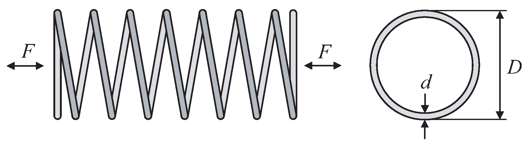
4.3. Optimal Design of Helical Compression Spring

The helical compression spring of Figure 5 is designed to support an axially-guided constant compressive load. This must be optimized to support a certain load without failure, with a minimum wire volume (minimum weight). The integer-valued number of spring coils (N), real-valued outside diameter of the spring (D), and spring wire diameter (d), which takes one of the allowable 42 discrete values given in

Table 4. Discrete allowable values of the spring wire diameter d.

Allowable Wire Diameter (in)
0.0090	0.0095	0.0104	0.0118	0.0128	0.0132	0.0140
0.0150	0.0162	0.0173	0.0180	0.0200	0.0230	0.0250
0.0280	0.0320	0.0350	0.0410	0.0470	0.0540	0.0630
0.0720	0.0800	0.0920	0.1050	0.1200	0.1350	0.1480
0.1620	0.1770	0.1920	0.2070	0.2250	0.2440	0.2630
0.2830	0.3070	0.3310	0.3620	0.3940	0.4375	0.5000

, are included as optimization variables and are set as $\mathit{x}={(x_1,x_2,x_3)}^T:={(D,N,d)}^T$. Accordingly, the objective function related to the minimization of the spring volume is formulated as

$$\underset{\mathit{x}}{min}f\left(\mathit{x}\right):=\frac{1}{4}{\pi }^2{x}_1{x}_3^2(x_2+2).$$

(22)

The following constraint conditions specify the design restrictions:

$$\begin{array}{cc}\hfill & {\displaystyle h_1\left(\mathit{x}\right):=\left(8cK{F}_{max}\right)/\left(\pi x_3^2\right)-S\le 0,K:=(4c-1)/(4c-4)+0.615/c,c:=x_1/x_3}\hfill \end{array}$$

(23)

$$\begin{array}{cc}\hfill & h_2\left(\mathit{x}\right):=l-l_{max}\le 0\hfill \end{array}$$

(24)

$$\begin{array}{cc}\hfill & h_3\left(\mathit{x}\right):=d_{min}-x_3\le 0\hfill \end{array}$$

(25)

$$\begin{array}{cc}\hfill & h_4\left(\mathit{x}\right):=(x_1+x_3)-D_{max}\le 0\hfill \end{array}$$

(26)

$$\begin{array}{cc}\hfill & h_5\left(\mathit{x}\right):=3.0-c\le 0,\hfill \end{array}$$

(27)

$$\begin{array}{cc}\hfill & h_6\left(\mathit{x}\right):={\delta }_p-{\delta }_{pm}\le 0,{\delta }_p:=F_p/k,k:=\left(G{x}_3^4\right)/\left(8x_2{c}^3\right)\hfill \end{array}$$

(28)

$$\begin{array}{cc}\hfill & h_7\left(\mathit{x}\right):={\delta }_p+\left(F_{max}-F_p\right)/k+1.05(x_2+2)x_3-l\le 0,l:=F_{max}/k+1.05(x_2+2)x_3\hfill \end{array}$$

(29)

$$\begin{array}{cc}\hfill & h_8\left(\mathit{x}\right):={\delta }_w-\left(F_{max}-F_p\right)/k\le 0\hfill \end{array}$$

(30)

The supplied numerical data included in the problem statement are listed in

Table 5. Parameter values used in the formulation of the helical compression spring problem.

Notation	Description	Value
$F_{max}$	Maximum working load	1000.0 (lb)
S	Maximum allowable shear stress	$1.89\times {10}^5$ (psi)
$l_{max}$	Maximum free length	14.0 (in)
$d_{min}$	Minimum wire diameter	0.2 (in)
$D_{max}$	Maximum outside spring diameter	3.0 (in)
$F_p$	Preload compression force	300.0 (lb)
${\delta }_{pm}$	Maximum allowable deflection	6.0 (in)
	under preload
${\delta }_w$	Deflection from preload position to	1.25 (in)
	maximum load position
G	Shear modulus of the material	$1.15\times {10}^7$ (psi)

, and the constraint details can be found in [1]. Combining the constraints $h_3\left(\mathit{x}\right)$-$h_5\left(\mathit{x}\right)$, the boundaries of $x_1$ and $x_2$ become $[0.6,3.0]$ and $[1,70]$, respectively, and the limits of $x_3$ are set automatically as $[0.0090,0.5000]$ from Table 4. We set the user parameters as $({\mathrm{D}}_{\mathrm{low}},{\mathrm{D}}_{\mathrm{high}},k_{\mathrm{DIV}})=(0.1,0.4,250)$.

This design problem was previously examined using various optimization algorithms including FA [1], PSO [2,14], DE [21], GA [38] and HSIA (hybrid swarm intelligence approach) [39]. The reported optimization performances, including statistical results, were compared in-depth with our PSO scheme, as presented in

Table 6. Optimization results of the helical compression spring design problem.

Reference Method	[40] NLPA a	[38] GA	[39] HSIA	[21] DE	[14] PSO	[1] FA	[2] PSO	Present Study PSO (${\mathit{n}}_{\mathit{s}}=16$)
$x_1$ (D)	1.180701	1.227411	1.223	1.223041	1.223041	1.223049	1.223041	1.223041
$x_2$ (N)	10	9	9	9	9	9	9	9
$x_3$ (d)	0.283	0.283	0.283	0.283	0.283	0.283	0.283	0.283
$-h_1\left({\mathit{x}}^{*}\right)$	5430.9	550.993	1008.81	1008.8114	1008.8114	1008.02	1008.8059	1008.811398
$-h_2\left({\mathit{x}}^{*}\right)$	8.8187	8.9264	8.946	8.94564	8.9456	8.946	8.945635	8.945636
$-h_3\left({\mathit{x}}^{*}\right)$	0.08298	0.0830	0.083	0.08300	0.083	0.083	0.083000	0.083000
$-h_4\left({\mathit{x}}^{*}\right)$	1.8193	1.7726	1.77696	1.77696	1.777	1.777	1.493959	1.493959
$-h_5\left({\mathit{x}}^{*}\right)$	1.1723	1.3371	1.32170	1.32170	1.3217	1.322	1.321700	1.321700
$-h_6\left({\mathit{x}}^{*}\right)$	5.4643	5.4585	5.4643	5.46429	5.4643	5.464	5.464286	5.464286
$-h_7\left({\mathit{x}}^{*}\right)$	0.0	0.0	0.0	0.0	0.0000	0	0.000000	0.000000
$-h_8\left({\mathit{x}}^{*}\right)$	0.0	0.0134	0.0	0.0	0.0000	0.0000	0.000010	0.000000
Best objective value	2.7995	2.6681	2.659	2.65856	2.65856	2.658576	2.658559	2.658559
Objective deviation	$1.0+5.301\times {10}^{-2}$	$1.0+3.589\times {10}^{-3}$	$1.0+1.659\times {10}^{-4}$	$1.0+3.761\times {10}^{-7}$	$1.0+3.761\times {10}^{-7}$	$1.0+6.394\times {10}^{-6}$	1.0	1.0
Worst objective value	N/A	N/A	N/A	N/A	N/A	7.8162919	N/A	2.660784
Average objective value	N/A	N/A	N/A	N/A	2.738024	4.3835958	N/A	2.658890
Standard deviation	N/A	N/A	N/A	N/A	N/A	4.6076313	N/A	0.000611
Function evaluations	N/A	N/A	N/A	26,000	15,000	75,000	4784–98,992	50,000

^a Nonlinear programming algorithm.

. In this table, it can be seen that our PSO scheme detected the best solution, satisfying all constraints; this was also reported in [2,14,21]. Among these, [14] found the best solution with a smaller number of function evaluations. However, in terms of statistical results, our PSO algorithm surpassed other conventional optimization methods with a reasonable number of function evaluations.

4.4. Optimal Design of Belleville Spring

This benchmark example is to design a Belleville spring of minimum weight, as shown in Figure 6. The four design variables are as follows: (1) thickness t ($=:x_1$), (2) height h ($=:x_2$), (3) internal diameter $D_i$ ($=:x_3$), and (4) external diameter $D_e$ ($=:x_4$). The cost function is given as:

$$\underset{\mathit{x}}{min}f\left(\mathit{x}\right):=0.07075\pi (x_4^2-x_3^2)x_1.$$

(31)

The constraints related to compressive stress, deflection, height to deflection, height to maximum height, outer diameter, inner diameter, and slope are formulated as

$$\begin{array}{cc}\hfill & h_1\left(\mathit{x}\right):=1000S-\frac{4E{\delta }_{max}}{(1-{\mu }^2)\alpha x_4^2}\left[\beta \left(x_2-\frac{{\delta }_{max}}{2}\right)+\gamma x_1\right]\ge 0,\hfill \end{array}$$

(32)

$$\begin{array}{cc}\hfill & h_2\left(\mathit{x}\right):={\left(\frac{4E{\delta }_{max}}{(1-{\mu }^2)\alpha x_4^2}\left[\left(x_2-\frac{\delta }{2}\right)\left(x_2-\delta \right)x_1+x_1^3\right]\right)}_{\delta ={\delta }_{max}}-P_{max}\ge 0,\hfill \end{array}$$

(33)

$$\begin{array}{cc}\hfill & h_3\left(\mathit{x}\right):={\delta }_l-{\delta }_{max}\ge 0,\hfill \end{array}$$

(34)

$$\begin{array}{cc}\hfill & h_4\left(\mathit{x}\right):=H-x_2-x_1\ge 0,\hfill \end{array}$$

(35)

$$\begin{array}{cc}\hfill & h_5\left(\mathit{x}\right):=D_{max}-x_4\ge 0,\hfill \end{array}$$

(36)

$$\begin{array}{cc}\hfill & h_6\left(\mathit{x}\right):=x_4-x_3\ge 0,\hfill \end{array}$$

(37)

$$\begin{array}{cc}\hfill & h_7\left(\mathit{x}\right):=0.3-\frac{x_2}{x_4-x_3}\ge 0,\hfill \end{array}$$

(38)

where

$$\begin{array}{cc}\hfill & \alpha =\frac{6}{\pi lnK}{\left(\frac{K-1}{K}\right)}^2,\beta =\frac{6}{\pi lnK}\left(\frac{K-1}{lnK}-1\right),\gamma =\frac{6}{\pi lnK}\left(\frac{K-1}{2}\right),\hfill \\ \hfill & P_{max}=5400\mathrm{lb},{\delta }_{max}=0.2\mathrm{in},\mu =0.3,S=200\mathrm{KPsi},H=2\mathrm{in},D_{max}=12.01\mathrm{in},\hfill \\ \hfill & K=x_4/x_3,{\delta }_l=g\left(a\right)x_2,a=x_2/x_1.\hfill \end{array}$$

The variation in $g\left(a\right)$ according to $a(=x_2/x_1)$ can be determined as shown in

Table 7. Variation of $g\left(a\right)$ with a.

a	≤1.4	1.5	1.6	1.7	1.8	1.9	2	2.1	2.2	2.3	2.4	2.5	2.6	2.7	≥2.8
$g\left(a\right)$	0.58	1	0.85	0.77	0.71	0.66	0.63	0.6	0.56	0.55	0.53	0.52	0.51	0.51	0.5

. We set the user parameters as $({\mathrm{D}}_{\mathrm{low}},{\mathrm{D}}_{\mathrm{high}},$$k_{\mathrm{DIV}})$$=(0.25,0.35,100)$.

A comparison of the best solution and statistical results for this design problem is presented in

Table 8. Optimization results of the Belleville spring design problem.

Reference Method	[42]	[43]		[41] OPTIVAR	[3] NBV	[30]		Present Study PSO (${\mathit{n}}_{\mathit{s}}=16$)
		GeneAS-I	GeneAS-II			ABC	TLBO
$x_1$ (t)	0.208	0.205	0.210	0.204	0.204143	N/A	0.204143	0.204143
$x_2$ (h)	0.2	0.201	0.204	0.200	0.2	N/A	0.2	0.200000
$x_3$ ($D_i$)	8.751	9.534	9.268	10.030	10.0304732	N/A	10.03047	10.030473
$x_4$ ($D_e$)	11.067	11.627	11.499	12.010	12.01	N/A	12.01	12.010000
$h_1\left({\mathit{x}}^{*}\right)$	2145.4109	−10.3396	2127.2624	134.0816	$4.58\times {10}^{-4}$	N/A	$1.77\times {10}^{-6}$	$6.93\times {10}^{-11}$
$h_2\left({\mathit{x}}^{*}\right)$	39.75018	2.8062	194.222554	−12.5328	$3.04\times {10}^{-7}$	N/A	$7.46\times {10}^{-8}$	$8.85\times {10}^{-10}$
$h_3\left({\mathit{x}}^{*}\right)$	0.00000	0.0010	0.0040	0.0000	$9.24\times {10}^{-10}$	N/A	$5.8\times {10}^{-11}$	$8.81\times {10}^{-13}$
$h_4\left({\mathit{x}}^{*}\right)$	1.592	1.5940	1.5860	1.5960	1.595856	N/A	1.595857	1.595857
$h_5\left({\mathit{x}}^{*}\right)$	0.943	0.3830	0.5110	0.0000	0	N/A	$2.35\times {10}^{-9}$	$1.58\times {10}^{-10}$
$h_6\left({\mathit{x}}^{*}\right)$	2.316	2.0930	2.2310	1.9800	1.979526	N/A	1.979527	1.979527
$h_7\left({\mathit{x}}^{*}\right)$	0.21364	0.20397	0.20856	0.19899	0.198965	N/A	0.198966	0.198966
Best objective value	2.121964	2.01807	2.16256	1.978715	1.979675	1.979675	1.979675	1.979675
Objective deviation	$1.0+7.187\times {10}^{-2}$	$1.0+1.939\times {10}^{-2}$	$1.0+9.238\times {10}^{-2}$	$1.0-4.849\times {10}^{-4}$	1.0	1.0	1.0	1.0
Feasibility	Feasible	Infeasible	Feasible	Infeasible	Feasible	N/A	Feasible	Feasible
Worst objective value	N/A	N/A	N/A	N/A	2.005431	2.104297	1.979757	1.979675
Average objective value	N/A	N/A	N/A	N/A	1.984698	1.995475	1.979688	1.979675
Standard deviation	N/A	N/A	N/A	N/A	7.78 $\times {10}^{-3}$	0.07	0.45	0.000000
Function evaluations	N/A	N/A	N/A	N/A	15,000	150,000	150,000	50,000

. It can be verified from this table that although three conventional methods (MBA, ABC, and TLBO) also found the optimal solution, the remarkable superiority of our PSO scheme to these optimizers is demonstrated by the worst, mean, and standard deviation values. It should be noted that the results of [41] seem to outperform ours in terms of optimal cost value; however, the solution was not feasible because the second constraint ($h_2\left(\mathit{x}\right)$) was violated.

4.5. Optimal Design of Speed Reducer

The design objective is to minimize the weight of the speed reducer of Figure 7, which is subject to constraints, including restrictions concerning the bending and surface stresses of the gear teeth, transverse deflection of the two shafts caused by the transmitted force, and stresses in the shafts. The decision variables, $x_1$ to $x_7$, represent, respectively, b (face width), m (tooth module), n (number of teeth on the pinion), $l_1$ (length of shaft 1 between bearings), $l_2$ (length of shaft 2 between bearings), $d_1$ (shaft diameter 1), and $d_2$ (diameter of shaft 2). Here, $x_3$ should take an integer value, while all the other variables are continuous.

The cost function then becomes

$$\begin{array}{cc}\hfill \underset{\mathit{x}}{min}f\left(\mathit{x}\right):=& 0.7854x_1{x}_2^2(3.3333x_3^2+14.9334x_3-43.0934)-1.508x_1(x_6^2+x_7^2)\hfill \\ \hfill & +7.4777(x_6^3+x_7^3)+0.7854(x_4{x}_6^2+x_5{x}_7^2).\hfill \end{array}$$

(39)

The following 11 constraint conditions result in the problem being highly complex:

$$\begin{array}{cc}\hfill & h_1\left(\mathit{x}\right):=27x_1^{-1}{x}_2^{-2}{x}_3^{-1}-1\le 0,\hfill \end{array}$$

(40)

$$\begin{array}{cc}\hfill & h_2\left(\mathit{x}\right):=397.5x_1^{-1}{x}_2^{-2}{x}_3^{-2}-1\le 0,\hfill \end{array}$$

(41)

$$\begin{array}{cc}\hfill & h_3\left(\mathit{x}\right):=1.93x_2^{-1}{x}_3^{-1}{x}_4^3{x}_6^{-4}-1\le 0,\hfill \end{array}$$

(42)

$$\begin{array}{cc}\hfill & h_4\left(\mathit{x}\right):=1.93x_2^{-1}{x}_3^{-1}{x}_5^3{x}_7^{-4}-1\le 0,\hfill \end{array}$$

(43)

$$\begin{array}{cc}\hfill & h_5\left(\mathit{x}\right):=\frac{\sqrt{{\left({\displaystyle \frac{745x_4}{x_2{x}_3}}\right)}^2+16.9\times {10}^6}}{0.1x_6^3}-1100\le 0,\hfill \end{array}$$

(44)

$$\begin{array}{cc}\hfill & h_6\left(\mathit{x}\right):=\frac{\sqrt{{\left({\displaystyle \frac{745x_5}{x_2{x}_3}}\right)}^2+157.5\times {10}^6}}{0.1x_7^3}-850\le 0,\hfill \end{array}$$

(45)

$$\begin{array}{cc}\hfill & h_7\left(\mathit{x}\right):=x_2{x}_3-40\le 0,\hfill \end{array}$$

(46)

$$\begin{array}{cc}\hfill & h_8\left(\mathit{x}\right):=5-x_1/x_2\le 0,\hfill \end{array}$$

(47)

$$\begin{array}{cc}\hfill & h_9\left(\mathit{x}\right):=x_1/x_2-12\le 0,\hfill \end{array}$$

(48)

$$\begin{array}{cc}\hfill & h_{10}\left(\mathit{x}\right):=(1.5x_6+1.9)x_4^{-1}-1\le 0,\hfill \end{array}$$

(49)

$$\begin{array}{cc}\hfill & h_{11}\left(\mathit{x}\right):=(1.1x_7+1.9)x_5^{-1}-1\le 0,\hfill \end{array}$$

(50)

where the limits of the variables are set as $2.6\le x_1\le 3.6$, $0.7\le x_2\le 0.8$, $17\le x_3\le 28$, $7.3\le x_4\le 8.3$, $7.3\le x_5\le 8.3$, $2.9\le x_6\le 3.9$, and $5.0\le x_7\le 5.5$. For this minimization problem, the performance of our PSO algorithm is compared with the extensive survey results presented in some articles [3,44,45] of the following six optimization methods: (i) DEDS: differential evolution with dynamic stochastic selection (ii) DELC: differential evolution with level comparison (iii) HEAA: hybrid evolutionary algorithm and adaptive constraint handling technique (iv) MDE: modified differential evolution (v) PSO-DE: PSO with differential evolution and (vi) MBA: mine blast algorithm (see [3] for details.). The user parameters were set as $({\mathrm{D}}_{\mathrm{low}},{\mathrm{D}}_{\mathrm{high}},k_{\mathrm{DIV}})=(0.25,0.35,100)$.

The optimization results are presented in

Table 9. Optimization results of the speed reducer design problem.

Reference Method	DEDS	DELC	HEAA	MDE	PSO-DE	MBA	Present Study PSO (${\mathit{n}}_{\mathit{s}}=16$)
$x_1$ (b)	3.5	3.5	3.500022	3.500010	3.5000000	3.500000	3.500000
$x_2$ (m)	0.7	0.7	0.70000039	0.70000	0.700000	0.700000	0.700000
$x_3$ (n)	17	17	17.000012	17	17.000000	17.000000	17.000000
$x_4$ ($l_1$)	7.3	7.3	7.300427	7.300156	7.300000	7.300033	7.300000
$x_5$ ($l_2$)	7.715319	7.715319	7.715377	7.800027	7.800000	7.715772	7.800000
$x_6$ ($d_1$)	3.350214	3.350214	3.350230	3.350221	3.350214	3.350218	2.900000
$x_7$ ($d_2$)	5.286654	5.286654	5.286663	5.286685	5.2866832	5.286654	5.286683
Best objective value	2994.471066	2994.471066	2994.499107	2996.356689	2996.348167	2994.482453	2896.259285
Objective deviation	$1.0+3.3910\times {10}^{-2}$	$1.0+3.3910\times {10}^{-2}$	$1.0+3.392\times {10}^{-2}$	$1.0+3.4561\times {10}^{-2}$	$1.0+3.4558\times {10}^{-2}$	$1.0+3.3914\times {10}^{-2}$	1.0
Worst objective value	2994.471066	2994.471066	2994.752311	2996.390137	2996.348204	2999.652444	2896.259380
Average objective value	2994.471066	2994.471066	2994.613368	2996.367220	2996.348174	2996.769019	2896.259292
Standard deviation	$3.6\times {10}^{-12}$	$1.9\times {10}^{-12}$	$7.0\times {10}^{-2}$	$8.2\times {10}^{-3}$	$6.4\times {10}^{-6}$	1.56	0.000017
Function evaluations	30,000	30,000	40,000	24,000	54,350	25,000	50,000

, which demonstrates that our PSO scheme outperformed some other optimization techniques in terms of precision (i.e., the lowest cost function value). For the detected best solution, the constraint values become $h_1\left({\mathit{x}}^{*}\right)=-0.073915$, $h_2\left({\mathit{x}}^{*}\right)=-0.197999$, $h_3\left({\mathit{x}}^{*}\right)=-0.107955$, $h_4\left({\mathit{x}}^{*}\right)=-0.904644$, $h_5\left({\mathit{x}}^{*}\right)=-534.994106$, $h_6\left({\mathit{x}}^{*}\right)=-0.000000$, $h_7\left({\mathit{x}}^{*}\right)=-28.100000$, $h_8\left({\mathit{x}}^{*}\right)=-0.000000$, $h_9\left({\mathit{x}}^{*}\right)=-7.000000$ $h_{10}\left({\mathit{x}}^{*}\right)=-0.143836$, and $h_{11}\left({\mathit{x}}^{*}\right)=-0.000000$, which demonstrates that all the constraint conditions are satisfied. Furthermore, it is observed in Table 9 that the proposed optimizer yields better results than those reported in the previous studies for the best, mean, and worst solutions, demonstrating the remarkable consistency of our optimization method.

4.6. Optimal Design of Stepped Cantilever Beam

This example considers a stepped cantilever beam subject to the end load shown in Figure 8 where minimizing the volume of the beam is the design objective. The height and width of the cross-sectional area in all five segments are taken as the design variables, which results in $\{x_1,x_3,x_5,x_7,x_9\}:=\{b_1,b_2,b_3,b_4,b_5\}$ and $\{x_2,x_4,x_6,x_8,x_{10}\}:=\{h_1,h_2,h_3,h_4,h_5\}$. Then, the objective function is formulated as:

$$\underset{\mathit{x}}{min}f\left(\mathit{x}\right):=100(x_1{x}_2+x_3{x}_4+x_5{x}_6+x_7{x}_8+x_9{x}_{10}),$$

(51)

where $x_1\in \{1,2,3,4,5\}$, $x_3,x_5\in \{2.4,2.6,2.8,3.1\}$, $x_2,x_4\in \{45,50,55,60\}$, $x_6\in \{30,31,\cdots ,65\}$, $1\le x_7,x_9\le 5$, and $30\le x_8,x_{10}\le 65$. The constraint conditions are described as follows. First, the bending stress in all segments must be less than the allowable limit of 14,000 (${\mathrm{N}/\mathrm{cm}}^2)$:

$$\begin{array}{cc}\hfill & h_1\left(\mathit{x}\right):=\frac{600P}{x_9{x}_{10}^2}-14,000\le 0,\hfill \end{array}$$

(52)

$$\begin{array}{cc}\hfill & h_2\left(\mathit{x}\right):=\frac{1200P}{x_7{x}_8^2}-14,000\le 0,\hfill \end{array}$$

(53)

$$\begin{array}{cc}\hfill & h_3\left(\mathit{x}\right):=\frac{1800P}{x_5{x}_6^2}-14,000\le 0,\hfill \end{array}$$

(54)

$$\begin{array}{cc}\hfill & h_4\left(\mathit{x}\right):=\frac{2400P}{x_3{x}_4^2}-14,000\le 0,\hfill \end{array}$$

(55)

$$\begin{array}{cc}\hfill & h_5\left(\mathit{x}\right):=\frac{3000P}{x_1{x}_2^2}-14,000\le 0,,\hfill \end{array}$$

(56)

where the concentrated load P = 50,000 (N). Second, the tip deflection of the cantilever beam must be smaller than the allowable limit of $2.7$ ($\mathrm{cm}$):

$$h_6\left(\mathit{x}\right):=\frac{{100}^{3}P}{3E}\left(\frac{1}{I_5}+\frac{7}{I_4}+\frac{19}{I_3}+\frac{37}{I_2}+\frac{61}{I_1}\right)-2.7\le 0,$$

(57)

where the elastic modulus of the material is $E=2\times {10}^7$ (${\mathrm{N}/\mathrm{cm}}^2$). Finally, the aspect ratio between the height and width of the cross section in each segment must be less than a value of 20:

$$\begin{array}{cc}\hfill & h_7\left(\mathit{x}\right):=\frac{x_{10}}{x_9}-20\le 0,\hfill \end{array}$$

(58)

$$\begin{array}{cc}\hfill & h_8\left(\mathit{x}\right):=\frac{x_8}{x_7}-20\le 0,\hfill \end{array}$$

(59)

$$\begin{array}{cc}\hfill & h_9\left(\mathit{x}\right):=\frac{x_6}{x_5}-20\le 0,\hfill \end{array}$$

(60)

$$\begin{array}{cc}\hfill & h_{10}\left(\mathit{x}\right):=\frac{x_4}{x_3}-20\le 0,\hfill \end{array}$$

(61)

$$\begin{array}{cc}\hfill & h_{11}\left(\mathit{x}\right):=\frac{x_2}{x_1}-20\le 0,.\hfill \end{array}$$

(62)

The user parameters of our PSO method were set as $({\mathrm{D}}_{\mathrm{low}},{\mathrm{D}}_{\mathrm{high}},k_{\mathrm{DIV}})=(5,10,100)$.

The best design variables and statistical results obtained via eight optimization methods are compared in

Table 10. Optimization results of the stepped cantilever beam design problem.

	Method	${\mathit{x}}_1$	${\mathit{x}}_2$	${\mathit{x}}_3$	${\mathit{x}}_4$	${\mathit{x}}_5$	${\mathit{x}}_6$	${\mathit{x}}_7$	${\mathit{x}}_8$	${\mathit{x}}_9$	${\mathit{x}}_{10}$	Objective Function				Function
		(${\mathit{b}}_{\mathbf{1}}$)	(${\mathit{h}}_{\mathbf{1}}$)	(${\mathit{b}}_{\mathbf{2}}$)	(${\mathit{h}}_{\mathbf{2}}$)	(${\mathit{b}}_{\mathbf{3}}$)	(${\mathit{h}}_{\mathbf{3}}$)	(${\mathit{b}}_{\mathbf{4}}$)	(${\mathit{h}}_{\mathbf{4}}$)	(${\mathit{b}}_{\mathbf{5}}$)	(${\mathit{h}}_{\mathbf{5}}$)	Best	Deviation	Worst	Mean	Std. Dev.	Evaluations
[46]	RNES 1 a	3	60	3.1	55	2.6	50	2.311	43.108	1.822	34.307	64269.594	$1.0+5.887\times {10}^{-3}$	N/A			12,000
	RNES 2	3	60	3.1	55	2.6	50	2.267	43.797	1.849	34.282	64322.433	$1.0+6.714\times {10}^{-3}$	N/A			12,000
	RNES 3	3	60	3.1	55	2.6	50	2.348	42.804	1.783	34.753	64299.108	$1.0+6.349\times {10}^{-3}$	N/A			12,000
	RNES 4	3	60	3.1	55	2.6	50	2.491	41.51	2.113	33.231	65416.896	$1.0+2.384\times {10}^{-2}$	N/A			12,000
[47]	DOT	N/A										65391.59	$1.0+2.345\times {10}^{-2}$	N/A			N/A
	SLP b	N/A										65451.50	$1.0+2.439\times {10}^{-2}$	N/A			N/A
	MLD c-SLP	N/A										65352.20	$1.0+2.283\times {10}^{-2}$	N/A			N/A
[48]	C/RU d	4	62	3.1	60	2.6	55	2.205	44.09	1.751	35.03	73555	$1.0+1.512\times {10}^{-1}$	N/A			N/A
	PD e	3	60	3.1	55	2.6	50	2.276	45.528	1.75	34.995	64537	$1.0+1.007\times {10}^{-2}$	N/A			N/A
	LAD f	3	60	3.1	55	2.6	50	2.262	45.233	1.75	34.995	64403	$1.0+7.975\times {10}^{-3}$	N/A			N/A
	CAD g	3	60	3.1	55	2.6	50	2.279	45.553	1.75	35.004	64558	$1.0+1.040\times {10}^{-2}$	N/A			N/A
[49]	GAOS Level 1	3	60	3.1	55	2.6	50	2.3	45.5	1.8	35	64815	$1.0+1.442\times {10}^{-2}$	N/A			10,000
	GAOS Level 2	3	60	3.1	55	2.6	50	2.27	45.25	1.75	35	64447	$1.0+8.664\times {10}^{-3}$	N/A			10,000
[50]	GA-APM h	3	60	3.1	55	2.6	50	2.2894	45.6256	1.7931	34.593	64698.56	$1.0+1.260\times {10}^{-2}$	73931.359	68107.046	N/A	35,000
[51]	AIS-GA	3	60	3.1	55	2.6	50	2.235	44.395	2.004	32.879	65559.60	$1.0+2.608\times {10}^{-2}$	77272.78	70857.12	N/A	35,000
	AIS-GA-C i	3	60	3.1	60	2.6	50	2.311	43.186	2.225	31.250	66533.47	$1.0+4.132\times {10}^{-2}$	76852.86	71821.69	N/A	35,000
[1]	FA	3	60	3.1	55	2.6	50	2.205	44.091	1.750	34.995	63893.52	$1.0+1.409\times {10}^{-6}$	64262.99420	64144.75312	175.91879	50,000
Present study	PSO ($n_s=16$)	3	60	3.1	55	2.6	50	2.20456	44.09111	1.74976	34.99514	63893.43	1.0	63893.43080	63893.43080	0.00000	50,000

^a Rank-niche evolution strategy. ^b Sequential linear programming. ^c Move limit definition. ^d Continuous/round up. ^e Precise discrete. ^f Linear approximate discrete. ^g Conservative approximate discrete. ^h Adaptive penalty method. ⁱ Clearing.

. This demonstrates that the proposed PSO scheme surpasses all other reported optimizers for finding the lowest cost function value. Furthermore, the mean and worst values achieved via our optimizer are considerably better than those reported in other studies. It is noteworthy that the zero standard deviation demonstrates the remarkable search precision and reliability of our optimization engine.

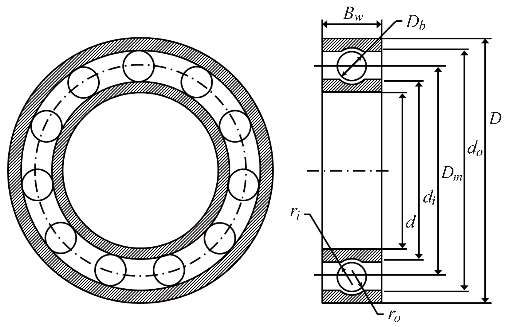
4.7. Optimal Design of Rolling Element Bearing

The design objective is to increase, as much as possible, the dynamic load-carrying capacity of the rolling element bearing in Figure 9. Five design variables are defined as follows; ball diameter ($D_b=:x_1$), pitch diameter ($D_m=:x_2$), number of balls ($Z=:x_3$), and inner and outer raceway curvature coefficients ($f_i=:x_4$ and $f_o=:x_5$). Note that other variables, such as $K_{Dmin}$ ($=:x_6$), $K_{Dmax}$ ($=:x_7$), $\epsilon$ ($=:x_8$), e ($=:x_9$), and $\zeta$ ($=:x_{10}$), appear only in the constraint conditions. Here, the number of balls $x_3$ should take an integer value whereas the remainders are taken as continuous values. The optimization problem is stated as

$$\underset{\mathit{x}}{max}f\left(\mathit{x}\right):=\left\{\begin{array}{cc}{C}_d=f_c{x}_5^{2/3}{x}_1^{1.8},\hfill & \mathrm{if}{x}_1\le 25.4\left(\mathrm{mm}\right),\hfill \\ C_d=3.647f_c{x}_5^{2/3}{x}_1^{1.4},\hfill & \mathrm{if}{x}_1>25.4\left(\mathrm{mm}\right),\hfill \end{array}\right.$$

(63)

subject to the following constraints that are derived from kinematic and manufacturing considerations:

$$\begin{array}{cc}\hfill & h_1\left(\mathit{x}\right):=\frac{{\varphi }_0}{2{sin}^{-1}(x_1/x_2)}-x_5+1\ge 0,\hfill \end{array}$$

(64)

$$\begin{array}{cc}\hfill & h_2\left(\mathit{x}\right):=2x_1-x_6(D-d)\ge 0,\hfill \end{array}$$

(65)

$$\begin{array}{cc}\hfill & h_3\left(\mathit{x}\right):=x_7(D-d)-2x_1\ge 0,\hfill \end{array}$$

(66)

$$\begin{array}{cc}\hfill & h_4\left(\mathit{x}\right):=x_{10}{B}_w-x_1\le 0,\hfill \end{array}$$

(67)

$$\begin{array}{cc}\hfill & h_5\left(\mathit{x}\right):=x_2-0.5(D+d)\ge 0,\hfill \end{array}$$

(68)

$$\begin{array}{cc}\hfill & h_6\left(\mathit{x}\right):=(0.5+x_9)(D+d)-x_2\ge 0,\hfill \end{array}$$

(69)

$$\begin{array}{cc}\hfill & h_7\left(\mathit{x}\right):=0.5(D-x_2-x_1)-x_8{x}_1\ge 0,\hfill \end{array}$$

(70)

$$\begin{array}{cc}\hfill & h_8\left(\mathit{x}\right):=x_3-0.515\ge 0,\hfill \end{array}$$

(71)

$$\begin{array}{cc}\hfill & h_9\left(\mathit{x}\right):=x_4-0.515\ge 0,\hfill \end{array}$$

(72)

where

$$\begin{array}{cc}\hfill & f_c=37.91{\left[1+{\left\{1.04{\left(\frac{1-\gamma }{1+\gamma }\right)}^{1.72}{\left(\frac{x_3(2x_4-1)}{x_4(2x_3-1)}\right)}^{0.41}\right\}}^{10/3}\right]}^{-0.3}\times \frac{{\gamma }^{0.3}{(1-\gamma )}^{1.39}}{{(1+\gamma )}^{1/3}}\times {\left[\frac{2x_3}{2x_3-1}\right]}^{0.41},\hfill \\ \hfill & {\varphi }_0=2\pi -2{cos}^{-1}\left(\frac{[{\{(D-d)/2-3(T/4)\}}^2+{\{D/2-T/4-x_1\}}^2-{\{d/2+T/4\}}^2]}{2\{(D-d)/2-3(T/4)\}\{D/2-T/4-x_1\}}\right),\hfill \\ \hfill & \gamma =\frac{x_1}{x_2},x_3=\frac{r_i}{x_1},x_4=\frac{r_o}{x_1},T=D-d-2x_1,D=160,d=90,B_w=30,\hfill \\ \hfill & r_i=r_o=11.033,0.5(D+d)\le x_2\le 0.6(D+d),0.15(D-d)\le x_1\le 0.45(D-d),\hfill \\ \hfill & 4\le x_5\le 50,0.515\le x_3,x_4\le 0.6,0.4\le x_6\le 0.5,0.6\le x_7\le 0.7,0.3\le x_8\le 0.4,\hfill \\ \hfill & 0.02\le x_9\le 0.1,0.6\le x_{10}\le 0.85.\hfill \end{array}$$

The simulation results using our PSO scheme are presented and compared with the results of other conventional methods in

Table 11. Optimization results of the rolling element bearing design problem.

Reference Method	[52] GA	[3] MBA	[30]		Present Study PSO (ns = 16)
			ABC	TLBO
$x_1$ ($D_b$)	125.7171	125.7153	N/A	125.7191	125.719056
$x_2$ ($D_m$)	21.423	21.423300	N/A	21.42559	21.425590
$x_3$ (Z)	11	11.000	N/A	11	11.000000
$x_4$ ($f_i$)	0.515	0.515000	N/A	0.515	0.515000
$x_5$ ($f_o$)	0.515	0.515000	N/A	0.515	0.515000
$x_6$ ($K_{Dmin}$)	0.4159	0.488805	N/A	0.424266	0.411776
$x_7$ ($K_{Dmax}$)	0.651	0.627829	N/A	0.633948	0.613510
$x_8$ ($\epsilon$)	0.300043	0.300149	N/A	0.3	0.300000
$x_9$ (e)	0.0223	0.097305	N/A	0.068858	0.059359
$x_{10}$ ($\zeta$)	0.751	0.646095	N/A	0.799498	0.667473
$h_1\left({\mathit{x}}^{*}\right)$	0.000821	0	N/A	0 a	0.000000
$h_2\left({\mathit{x}}^{*}\right)$	13.732999	8.630183	N/A	13.15257	14.026828
$h_3\left({\mathit{x}}^{*}\right)$	2.724000	1.101429	N/A	1.5252	0.094509
$h_4\left({\mathit{x}}^{*}\right)$	−1.107	2.040448	N/A	0.719056	−1.401405
$h_5\left({\mathit{x}}^{*}\right)$	0.717000	0.715366	N/A	16.49544	0.719056
$h_6\left({\mathit{x}}^{*}\right)$	4.857899	23.611002	N/A	0	14.120649
$h_7\left({\mathit{x}}^{*}\right)$	0.0021	0.000480	N/A	0	0.000000
$h_8\left({\mathit{x}}^{*}\right)$	0.000007	0	N/A	2.559363	0.000000
$h_9\left({\mathit{x}}^{*}\right)$	0.000007	0	N/A	0	0.000000
Best objective value	81,843.3	85,535.9611 b	81,859.7416	81,859.74	81,859.7416
Objective deviation	$1.0-2.009\times {10}^{-4}$	$1.0+4.491\times {10}^{-2}$	1.0	$1.0-1.955\times {10}^{-8}$	1.0
Feasibility	Feasible	Infeasible	N/A	Infeasible	Feasible
Worst objective value	N/A	84,440.1948	78,897.81	80,807.8551	81,859.7401
Average objective value	N/A	85,321.4030	81,496	81,438.987	81,859.7415
Standard deviation	N/A	211.52	0.69	0.66	0.0003
Function evaluations	225,000	50,000	10,000	10,000	50,000

^a Some constraint function values do not coincide with those calculated using the provided optimal solution. Their solution provides $h_1\left({\mathit{x}}^{*}\right)=0.000004$, $h_2\left({\mathit{x}}^{*}\right)=13.152560$, $h_3\left({\mathit{x}}^{*}\right)=1.525180$, $h_4\left({\mathit{x}}^{*}\right)=2.559350$, $h_5\left({\mathit{x}}^{*}\right)=0.719100$, $h_6\left({\mathit{x}}^{*}\right)=16.495400$, $h_7\left({\mathit{x}}^{*}\right)=-0.000022$, $h_8\left({\mathit{x}}^{*}\right)=0.0$, and $h_9\left({\mathit{x}}^{*}\right)=0.0$. ^b This best value does not coincide with that calculated using the provided optimal solution. Their solution provides $f\left({\mathit{x}}^{*}\right)=81843.68625$.

. The user parameters of the PSO method were set as $({\mathrm{D}}_{\mathrm{low}},{\mathrm{D}}_{\mathrm{high}},k_{\mathrm{DIV}})=(0.3,0.5,100)$. Although the reported best objective function value of TLBO in [30] is identical to ours, their solution does not satisfy the given constraint conditions. It should be noted that the constraint function values given in [30] cannot be obtained from their optimal solution. However, [3] reported the best cost function value of $85535.9611$ but their optimal solution provides $f\left({\mathit{x}}^{*}\right)=81843.68625$, which is a lower value than ours. Furthermore, the constraint function value presented by [3] demonstrates that their method produced an infeasible solution. Among the compared studies, a feasible solution was obtained by [52]; however, our optimization scheme surpassed their method, having remarkable precision and an acceptable number of function evaluations.

4.8. Car Side Impact Design Problem

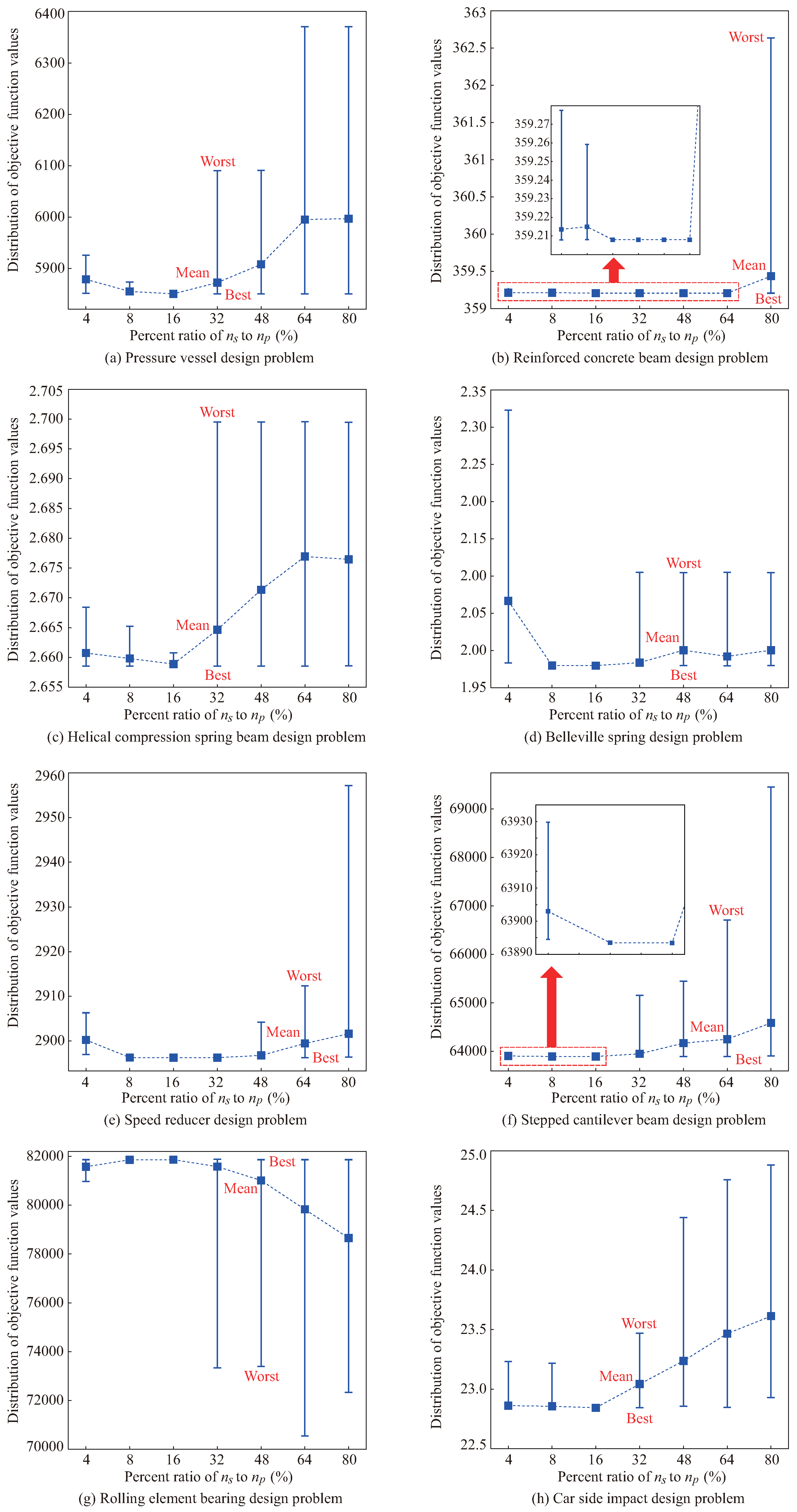
This problem addresses the case of an automobile side impact. Its objective is to improve the side impact crash performance while reducing the total weight of the automobile. Figure 10 illustrates the finite element model of the automobile, which is adopted from [1]. This problem contains eleven variables, such as the thickness of the B-Pillar inner ($x_1$), B-Pillar reinforcement ($x_2$), floor side inner ($x_3$), cross members ($x_4$), door beam ($x_5$), door belt line reinforcement ($x_6$), roof rail ($x_7$), materials of B-pillar inner and floor side inner ($x_8$ and $x_9$), and barrier height and hitting position ($x_{10}$ and $x_{11}$). Nine design variables are continuous ($x_{\ell },\ell =1,2,\cdots ,7,10,11$), and $x_8$ and $x_9$ are discrete. This optimal design problem is formulated as

$$\underset{\mathit{x}}{min}f\left(\mathit{x}\right):=1.98+4.90x_1+6.67x_2+6.98x_3+4.01x_4+1.78x_5+2.73x_7,$$

(73)

subject to

$$\begin{array}{cc}\hfill & h_1\left(\mathit{x}\right)=F_a\left(\mathrm{load\; in\; the\; abdomen}\right)\le 1\left(\mathrm{kN}\right),\hfill \end{array}$$

(74)

$$\begin{array}{cc}\hfill & h_2\left(\mathit{x}\right):=V{C}_u\left(\mathrm{dummy\; upper\; chest}\right)\le 0.32\left(\mathrm{m}/\mathrm{s}\right),\hfill \end{array}$$

(75)

$$\begin{array}{cc}\hfill & h_3\left(\mathit{x}\right):=V{C}_m\left(\mathrm{dummy\; middle\; chest}\right)\le 0.32\left(\mathrm{m}/\mathrm{s}\right),\hfill \end{array}$$

(76)

$$\begin{array}{cc}\hfill & h_4\left(\mathit{x}\right):=V{C}_l\left(\mathrm{dummy\; lower\; chest}\right)\le 0.32\left(\mathrm{m}/\mathrm{s}\right),\hfill \end{array}$$

(77)

$$\begin{array}{cc}\hfill & h_5\left(\mathit{x}\right):={\Delta }_{ur}\left(\mathrm{upper\; rib\; deflection}\right)\le 32\left(\mathrm{mm}\right),\hfill \end{array}$$

(78)

$$\begin{array}{cc}\hfill & h_6\left(\mathit{x}\right):={\Delta }_{mr}\left(\mathrm{middle\; rib\; deflection}\right)\le 32\left(\mathrm{mm}\right),\hfill \end{array}$$

(79)

$$\begin{array}{cc}\hfill & h_7\left(\mathit{x}\right):={\Delta }_{lr}\left(\mathrm{lower\; rib\; deflection}\right)\le 32\left(\mathrm{mm}\right),\hfill \end{array}$$

(80)

$$\begin{array}{cc}\hfill & h_8\left(\mathit{x}\right):=F_p\left(\mathrm{public\; force}\right)\le 4\left(\mathrm{kN}\right),\hfill \end{array}$$

(81)

$$\begin{array}{cc}\hfill & h_9\left(\mathit{x}\right):=V_{MBP}\left(\mathrm{velocity\; of\; V-Pillar\; at\; the\; middle\; point}\right)\le 9.9\left(\mathrm{mm}/\mathrm{ms}\right),\hfill \end{array}$$

(82)

$$\begin{array}{cc}\hfill & h_{10}\left(\mathit{x}\right):=V_{FD}\left(\mathrm{velocity\; of\; front\; door\; at\; V-Pillar}\right)\le 15.7\left(\mathrm{mm}/\mathrm{ms}\right),\hfill \end{array}$$

(83)

where

$$\begin{array}{cc}\hfill & F_a=1.16-0.3717x_2{x}_4-0.00931x_2{x}_{10}-0.484x_3{x}_9+0.01343x_6{x}_{10}\hfill \end{array}$$

(84)

$$\begin{array}{cc}\hfill & V{C}_u=0.261-0.0159x_1{x}_2-0.188x_1{x}_8-0.019x_2{x}_7+0.0144x_3{x}_5+0.0008757x_5{x}_{10}\hfill \\ \hfill & +0.08045x_6{x}_9+0.00139x_8{x}_{11}+0.00001575x_{10}{x}_{11}\hfill \end{array}$$

(85)

$$\begin{array}{cc}\hfill & V{C}_m=0.214+0.00817x_5-0.131x_1{x}_8-0.0704x_1{x}_9+0.03099x_2{x}_6-0.018x_2{x}_7\hfill \\ \hfill & +0.0208x_3{x}_8+0.121x_3{x}_9-0.00364x_5{x}_6+0.0007715x_5{x}_{10}-0.0005354x_6{x}_{10}\hfill \\ \hfill & +0.00121x_8{x}_{11}+0.00184x_9{x}_{10}-0.02x_2^2\hfill \end{array}$$

(86)

$$\begin{array}{cc}\hfill & V{C}_l=0.74-0.61x_2-0.163x_3{x}_8+0.001232x_3{x}_{10}-0.166x_7{x}_9+0.227x_2^2\hfill \end{array}$$

(87)

$$\begin{array}{cc}\hfill & {\Delta }_{ur}=28.98+3.818x_3-4.2x_1{x}_2+0.0207x_5{x}_{10}+6.63x_6{x}_9-7.7x_7{x}_8+0.32x_9{x}_{10}\hfill \end{array}$$

(88)

$$\begin{array}{cc}\hfill & {\Delta }_{mr}=33.86+2.95x_3+0.1792x_{10}-5.057x_1{x}_2-11.0x_2{x}_8-0.0215x_5{x}_{10}-9.98x_7{x}_8+22.0x_8{x}_9\hfill \end{array}$$

(89)

$$\begin{array}{cc}\hfill & {\Delta }_{lr}=46.36-9.9x_2-12.9x_1{x}_8+0.1107x_3{x}_{10}\hfill \end{array}$$

(90)

$$\begin{array}{cc}\hfill & F_p=4.72-0.5x_4-0.19x_2{x}_3-0.0122x_4{x}_{10}+0.009325x_6{x}_{10}+0.000191x_{11}^2\hfill \end{array}$$

(91)

$$\begin{array}{cc}\hfill & V_{MBP}=10.58-0.674x_1{x}_2-1.95x_2{x}_8+0.02054x_3{x}_{10}-0.0198x_4{x}_{10}+0.028x_6{x}_{10}\hfill \end{array}$$

(92)

$$\begin{array}{cc}\hfill & V_{FD}=16.45-0.489x_3{x}_7-0.843x_5{x}_6+0.0432x_9{x}_{10}-0.0556x_9{x}_{11}-0.000786x_{11}^2.\hfill \end{array}$$

(93)

The simple bounds of the design variables are $0.5\le x_1,x_2,x_3,x_4,x_5,x_6,x_7\le 1.5$, $-30\le x_{10},x_{11}\le 30$, and two discrete type variables are $x_8,x_9\in \{0.192,0.345\}$.

Table 12. Optimization results of the car side impact design problem.

Reference Method	[1]				Present Study PSO (${\mathit{n}}_{\mathit{s}}=16$)
	PSO	DE	GA	FA
$x_1$	0.50000	0.50000	0.50005	0.50000	0.500000
$x_2$	1.11670	1.11670	1.28017	1.36000	1.116366
$x_3$	0.50000	0.5000	0.50001	0.50000	0.500000
$x_4$	1.30208	1.30208	1.03302	1.20200	1.302197
$x_5$	0.50000	0.50000	0.50001	0.50000	0.500000
$x_6$	1.50000	1.50000	0.50000	1.12000	1.500000
$x_7$	0.50000	0.50000	0.50000	0.50000	0.500000
$x_8$	0.34500	0.34500	0.34994 a	0.34500	0.345000
$x_9$	0.19200	0.19200	0.19200	0.19200	0.192000
$x_{10}$	−19.54935	−19.54935	10.3119	8.87307	−19.561544
$x_{11}$	−0.00431	−0.00431	0.00167	−18.99808	−0.000190
Best objective value	22.84474	22.84298 b	22.85653	22.84298 c	22.842969
Objective deviation	$1.0+7.753\times {10}^{-5}$	$1.0+4.815\times {10}^{-7}$	$1.0+5.937\times {10}^{-4}$	$1.0+4.815\times {10}^{-7}$	1.0
Feasibility	Feasible	Feasible	Infeasible	Infeasible	Feasible
Worst objective value	23.21354	24.12606	26.240578	24.06623	22.846465
Average objective value	22.89429	23.22828	23.51585	22.89376	22.843136
Standard deviation	0.15017	0.34451	0.66555	0.16667	0.000649

^a$x_8\notin \{0.192,0.345\}.$^b The optimal solution is identical to that of PSO but different objective function values are provided in Gandomi et al. [1]. ^c This best value does not coincide with that calculated using the provided optimal solution, $f\left({\mathit{x}}^{*}\right)=24.06622$. Furthermore, their optimal solution may not guarantee the satisfaction of two constraint conditions, $h_8\left({\mathit{x}}^{*}\right)$ = 4.02129 > 4 kN and $h_{10}\left(\mathit{x}\right)$ = 15.84839 > 15.7 mm/ms.

compares the best solution and the statistical results of the proposed method and other reported methods. The user parameters of our PSO method were set as $({\mathrm{D}}_{\mathrm{low}},{\mathrm{D}}_{\mathrm{high}},k_{\mathrm{DIV}})=(0.01,0.03,200)$. This table shows that our optimization scheme produced the lowest cost function value together with a highly reliable performance, which is confirmed from the worst, mean, and standard deviation values. In particular, the superiority of our optimizer to the recently developed FA method in [1] is in the objective function values and constrained accuracy performance.

4.9. Discussions

The statistical results corresponding to the different percent ratio of $n_s$ to $n_p$ for the numerical examples in the previous sections are given in Figure 11. This figure verifies that a remarkable optimization accuracy and reliability can be achieved when the ratio $n_s/n_p$ is approximately $10\%$. However, the worst solution and standard deviation were most strongly dependent on the value of $n_s$ (see the cases of $n_s/n_p\le 4\%$ and $n_s/n_p\ge 32\%$). The above findings can be explained as follows. As illustrated in Figure 1, each particle evolves based only on the local information of the neighbors. The amount of information becomes more limited as the ratio of $n_s$ to $n_p$ decreases. Therefore, the low $n_s$/$n_p$ results in the tardy propagation of the successful social-best search result by a certain particle to particles belonging to other subpopulations. Such a case may lead to a slow convergence rate of the swarm toward an optimal solution while reducing the risk of the particles prematurely converging. This fact implies that more iterations could be required to guarantee the convergence of particles to a global optimum. In contrast, a high ratio of $n_s$ to $n_p$ implies that a particle obtains a large amount of information from several other neighboring particles. Therefore, a high convergence rate may be achieved despite the high risk of a fatal premature convergence phenomenon occurring, which usually causes the performance consistency of the optimizer to deteriorate. Figure 12 illustrates the convergence characteristics of $f_{min}^k:=min\left\{f\left({\mathit{x}}_1^k\right),f\left({\mathit{x}}_2^k\right),\cdots ,f\left({\mathit{x}}_{n_p}^k\right)\right\}$ for all 30 independent runs. Here, “Modified ATRE-PSO" refers to the method in which the original ATRE-PSO of [23,27] and our constraint handling scheme are combined, which is identical to the proposed PSO method with $n_s/n_p=100\%$ (i.e., star topology). The figure shows that the proposed cyclic network-based PSO method converged to the near-optimal solution in every run of the algorithm as compared with the star topology-based method. This improved reliability was achieved in all the considered design problems and thus can be considered a superiority of the optimization capability of the proposed method.

5. Conclusions

This study presented the realization of an easy-to-use diversity-guided PSO methodology for engineering optimal design problems with MIDC variables and subject to various real-life physical constraints. This scheme uses diversity classifiers for cyclically neighboring subpopulations and is characterized by superior reliability and validity. This PSO strategy combined two kinds of diversity-enhancing mechanisms. The first diversity-boosting tool was to construct cyclically neighboring multisubpopulations, one for each particle (host particle), where the host particle interacts only with a limited number of nearby neighbor particles during the search process. In this structure, information on the good fitness value of one host particle is cyclically propagated to other neighboring host particles during the evolution process. Therefore, this structure enforces each particle to achieve social learning from its respective neighborhoods and not directly from the best position of the entire swarm, which results in the enhancement of population diversity. The second diversity improvement for each subpopulation was to extend the above PSO mechanism to be combined with the idea of the three-phase velocity update law for governing the behavior of the host particle. In this extended PSO algorithm, the velocity behavior of each host particle per iteration is governed by either attraction, repulsion, or in-between phases, chosen according to the diversity classifier applied to the subpopulation of the host particle. In summary, our PSO scheme not only exploits the constricted social learning of each particle through cyclically neighboring subpopulations but also incorporates the three-phase velocity behavior law implemented by following the locally distributed diversity measures categorized for each subpopulation. This novel PSO scheme features high reliability, as well as superior practicality for engineering optimization problems involving MIDC variables, which are handled via the straightforward rounding-off technique that has been widely adopted in swarm-inspired metaheuristic search technologies. Several benchmark MIDC design problems were investigated in-depth, clearly verifying that the proposed PSO scheme is a highly useful tool, providing remarkable reliability.

References

1. Gandomi, A.H.; Yang, X.-S.; Alavi, A.H. Mixed variable structural optimization using firefly algorithm. Comput. Struct. 2011, 89, 2325–2336. [Google Scholar] [CrossRef]
2. Datta, D.; Figueira, J.R. A real-integer-discrete-coded particle swarm optimization for design problems. Appl. Soft Comput. 2011, 11, 3625–3633. [Google Scholar] [CrossRef]
3. Sadollaha, A.; Bahreininejada, A.; Eskandarb, H.; Hamdia, M. Mine blast algorithm: A new population based algorithm for solving constrained engineering optimization problems. Appl. Soft Comput. 2013, 13, 2592–2612. [Google Scholar] [CrossRef]
4. Banks, A.; Vincent, J.; Anyakoha, C. A review of particle swarm optimization. Part I: Background and development. Nat. Comput. 2007, 6, 467–484. [Google Scholar] [CrossRef]
5. Banks, A.; Vincent, J.; Anyakoha, C. A review of particle swarm optimization. Part II: Hybridisation, combinatorial, multicriteria and constrained optimization, and indicative applications. Nat. Comput. 2007, 7, 109–124. [Google Scholar] [CrossRef]
6. Tomassetti, G. A cost-effective algorithm for the solution of engineering problems with particle swarm optimization. Eng. Optim. 2010, 42, 471–495. [Google Scholar] [CrossRef] [Green Version]
7. Pulido, G.T.; Coello, C.A.C. A constraint-handling mechanism for particle swarm optimization. In Proceedings of the 2004 Congress on Evolutionary Computation, Portland, OR, USA, 19–23 June 2004; pp. 1396–1403. [Google Scholar]
8. Parsopoulos, K.E.; Vrahatis, M.N. Unified particle swarm optimization for solving constrained engineering optimization problems. In Advances in Natural Computation; Springer: Berlin/Heidelberg, Germany, 2005; pp. 582–591. [Google Scholar]
9. Mezura-Montes, E.; Coello Coello, C.A. Constraint-handling in nature-inspired numerical optimization: Past, present and future. Swarm Evol. Comput. 2011, 1, 173–194. [Google Scholar] [CrossRef]
10. Chun, S.; Kim, Y.-T.; Kim, T.-H. A diversity-enhanced constrained particle swarm optimizer for mixed integer-discrete-continuous engineering design problems. Adv. Mech. Eng. 2013, 2013, 130750-1–130750-11. [Google Scholar] [CrossRef] [Green Version]
11. Das, S.; Suganthan, P.N. Differential evolution: A survey of the state-of-the-art. IEEE Trans. Evol. Comput. 2011, 15, 4–31. [Google Scholar] [CrossRef]
12. Parsopoulos, K.E.; Vrahatisy, M.N. Recent approaches to global optimization problems through particle swarm optimization. Nat. Comput. 2002, 1, 235–306. [Google Scholar] [CrossRef]
13. Coelho, L.S. An efficient particle swarm approach for mixed-integer programming in reliability-redundancy optimization applications. Reliab. Eng. Syst. Saf. 2009, 94, 830–837. [Google Scholar] [CrossRef]
14. He, S.; Prempain, E.; Wu, Q.H. An improved particle swarm optimizer for mechanical design optimization problems. Eng. Optim. 2004, 36, 585–605. [Google Scholar] [CrossRef]
15. Venter, G.; Sobieski, J.S. Particle swarm optimization. AIAA J. 2003, 41, 1583–1589. [Google Scholar] [CrossRef] [Green Version]
16. Venter, G.; Sobieski, J.S. Multidisciplinary optimization of a transport aircraft wing using particle swarm optimization. Struct. Multidiscip. Optim. 2004, 26, 121–131. [Google Scholar] [CrossRef] [Green Version]
17. Akhtar, S.; Tai, K.; Ray, T. A socio-behavioural simulation model for engineering design optimization. Eng. Optim. 2002, 34, 341–354. [Google Scholar] [CrossRef]
18. Cagnina, L.C.; Esquivel, S.C.; Coello Coello, C.A. Solving engineering optimization problems with the simple constrained particle swarm optimizer. Informatica 2008, 32, 319–325. [Google Scholar]
19. Coello, C.A.C. Use of a self-adaptive penalty approach for engineering optimization problems. Comput. Ind. 2000, 41, 113–127. [Google Scholar] [CrossRef]
20. Hu, X.; Eberhart, R.C.; Shi, Y. Engineering optimization with particle swarm. In Proceedings of the 2003 the IEEE Swarm Intelligence Symposium, Indianapolis, IN, USA, 24–26 April 2003; pp. 53–57. [Google Scholar]
21. Lampinen, J.; Zelinka, I. Mixed-integer-discrete-continuous optimization by differential evolution. Part 2. A practical example. In Fifth International Mendel Conference on Soft Computing (MENDEL’99); Brno University of Technology: Brno, Czech Republic, 1999; pp. 77–81. [Google Scholar]
22. Liu, H.; Abraham, A.; Zhang, W. A fuzzy adaptive turbulent particle swarm optimization. Int. J. Innov. Comput. Appl. 2007, 1, 39–47. [Google Scholar] [CrossRef]
23. Pant, M.; Thangaraj, R.; Abraham, A. Particle swarm optimization: Performance tuning and empirical analysis. In Foundations of Computational Intelligence Volume 3: Global Optimization; Springer: Berlin/Heidelberg, Germany, 2009; pp. 101–128. [Google Scholar]
24. Lane, J.; Engelbrecht, A.; Gain, J. Particle swarm optimization with spatially meaningful neighbours. In Proceedings of the 2008 IEEE Swarm Intelligence Symposium, St. Louis, MO, USA, 21–23 September 2008; pp. 1–8. [Google Scholar]
25. Richards, M.; Ventura, D. Dynamic sociometry in particle swarm optimization. In Proceedings of the Sixth International Conference on Computational Intelligence and Natural Computing, Cary, NC, USA, 26–30 September 2003; pp. 1557–1560. [Google Scholar]
26. Mendes, R.; Neves, J. What makes a successful society? Experiments with population topologies in particle swarms. Lect. Notes Comput. Sci. 2004, 3171, 346–355. [Google Scholar]
27. Pant, M.; Radha, T.; Singh, V.P. A simple diversity guided particle swarm optimization. In Proceedings of the 2007 IEEE Congress on Evolutionary Computation, Singapore, 25–28 September 2007; pp. 3294–3299. [Google Scholar]
28. Maruta, I.; Kim, T.-H.; Song, D.H.; Sugie, T. Synthesis of fixed-structure robust controllers using a constrained particle swarm optimizer with cyclic neighborhood topology. Expert Syst. Appl. 2013, 40, 3595–3605. [Google Scholar] [CrossRef]
29. Zavala, A.E.M.; Aguirre, A.H.; Diharce, E.V. Robust PSO-based constrained optimization by perturbing the particle’s memory. In Swarm Intelligence: Focus on Ant and Particle Swarm Optimization; I-Tech Education and Publishing: Chicago, IL, USA, 2007; pp. 57–76. [Google Scholar]
30. Rao, R.V.; Savsani, V.J.; Vakharia, D.P. Teaching-learning-based optimization: A novel method for constrained mechanical design optimization problems. Comput.-Aided Des. 2011, 43, 303–315. [Google Scholar] [CrossRef]
31. Mahdavi, M.; Fesanghary, M.; Damangir, E. An improved harmony search algorithm for solving optimization problems. Appl. Math. Comput. 2007, 188, 1567–1579. [Google Scholar] [CrossRef]
32. Dimopoulos, G.G. Mixed-variable engineering optimization based on evolutionary and social metaphors. Comput. Methods Appl. Mech. Eng. 2007, 196, 803–817. [Google Scholar] [CrossRef]
33. Hedar, A.R.; Fukushima, M. Derivative-free filter simulated annealing method for constrained continuous global optimization. J. Glob. Optim. 2005, 35, 521–649. [Google Scholar] [CrossRef]
34. Amir, H.M.; Hasegawa, T. Nonlinear mixed-discrete structural optimization. J. Struct. Eng. 1898, 115, 626–646. [Google Scholar] [CrossRef]
35. Shih, C.J.; Yang, Y.C. Generalized Hopfield network based structural optimization using sequential unconstrained minimization technique with additional penalty strategy. Adv. Eng. Softw. 2002, 33, 721–729. [Google Scholar] [CrossRef]
36. Mezura-Montes, E.; Hernandez-Ocana, B. Modified bacterial foraging optimization for engineering design. In Intelligent Engineering Systems through Artificial Neural Networks; ASME Press (eBook): New York, NY, USA, 2009; Volume 19, pp. 357–364. [Google Scholar]
37. Yun, Y.S. Study on Adaptive Hybrid Genetic Algorithm and Its Applications to Engineering Design Problems. Master’s Thesis, Waseda University, Tokyo, Japan, 2005. [Google Scholar]
38. Wu, S.-J.; Chow, P.-T. Genetic algorithms for nonlinear mixed discrete-integer optimization problems via meta-genetic parameter optimization. Eng. Optim. 1995, 24, 137–159. [Google Scholar] [CrossRef]
39. Guo, C.; Hu, J.; Ye, B.; Cao, Y. Swarm intelligence for mixed-variable design optimization. J. Zhejiang Univ. Sci. 2004, 5, 851–860. [Google Scholar] [CrossRef] [Green Version]
40. Sandgren, E. Nonlinear integer and discrete programming in mechanical design optimization. ASME J. Mech. Des. 1990, 112, 223–229. [Google Scholar] [CrossRef]
41. Siddall, J.N. Optimal Engineering Design: Principles and Applications; CRC Press: New York, NY, USA, 1982. [Google Scholar]
42. Coello, C.A.C. Treating constraints as objectives for single-objective evolutionary optimization. Eng. Optim. 2000, 32, 275–308. [Google Scholar] [CrossRef]
43. Deb, K. GeneAS: A robust optimal design technique for mechanical component design. In Evolutionary Algorithms in Engineering Applications; Springer: Berlin/Heidelberg, Germany, 1997; pp. 497–514. [Google Scholar]
44. Liu, H.; Cai, Z.; Wang, Y. Hybridizing particle swarm optimization with differential evolution for constrained numerical and engineering optimization. Appl. Soft Comput. 2010, 10, 629–640. [Google Scholar] [CrossRef]
45. Wang, L.; Li, L.P. An effective differential evolution with level comparison for constrained engineering design. Struct. Multidiscip. Optim. 2010, 41, 947–963. [Google Scholar] [CrossRef]
46. Chen, T.Y.; Chen, H.C. Mixed-discrete structural optimization using a rank-niche evolution strategy. Eng. Optim. 2009, 41, 39–58. [Google Scholar] [CrossRef]
47. Lamberti, L.; Pappalettere, C. Move limits definition in structural optimization with sequential linear programming. Part II: Numerical examples. Comput. Structres 2003, 81, 215–238. [Google Scholar] [CrossRef]
48. Thanedar, P.B.; Vanderplaats, G.N. Survey of discrete variable optimization for structural design. J. Struct. Eng. 1995, 121, 301–306. [Google Scholar] [CrossRef]
49. Erbatur, F.; Hasancebi, O.; Tutuncu, I.; Kilic, H. Optimal design of planar and space structures with genetic algorithms. Comput. Structres 2000, 75, 209–224. [Google Scholar] [CrossRef]
50. Lemonge, A.C.C.; Barbosa, H.J.C. An adaptive penalty scheme for genetic algorithms in structural optimization. Int. J. Numer. Methods Eng. 2004, 59, 703–736. [Google Scholar] [CrossRef]
51. Bernardino, H.S.; Barbosa, H.J.C.; Lemonge, A.C.C. A hybrid genetic algorithm for constrained optimization problems in mechanical engineering. In Proceedings of the 2007 IEEE Congress on Evolutionary Computation, Singapore, 25–28 September 2007; pp. 646–653. [Google Scholar]
52. Gupta, S.; Tiwari, R.; Shivashankar, B.N. Multi-objective design optimization of rolling bearings using genetic algorithm. Mech. Mach. Theory 2007, 42, 1418–1443. [Google Scholar] [CrossRef]
Figure 1. Schematic diagram of the proposed diversity-guided particle swarm optimizer (PSO) with a cyclic network mechanism.
Mathematics 08 02016 g001
Figure 2. Flowchart of the PSO scheme with a diversity classifier for cyclically neighboring subpopulations for solving the constrained MIDC optimization problems.
Mathematics 08 02016 g002
Figure 3. Configuration of a pressure vessel.
Mathematics 08 02016 g003
Figure 4. Configurationof a reinforced concrete beam.
Mathematics 08 02016 g004
Figure 5. Configuration of a helical compression spring.
Mathematics 08 02016 g005
Figure 6. Configuration of a Belleville spring.
Mathematics 08 02016 g006
Figure 7. Configuration of a speed reducer.
Mathematics 08 02016 g007
Figure 8. Configuration of a stepped cantilever beam.
Mathematics 08 02016 g008
Figure 9. Configuration of a rolling element bearing.
Mathematics 08 02016 g009
Figure 10. Finite element model utilized in the car side impact problem [1].
Mathematics 08 02016 g010
Figure 11. Distributions of f ( x * ) corresponding to n s / n p for eight numerical examples.
Mathematics 08 02016 g011
Figure 12. Convergence behaviors of f ( x * ) for eight numerical examples.
Mathematics 08 02016 g012