On Three Constructions of Nanotori

Abstract

There are three different approaches for constructing nanotori in the literature: one with three parameters suggested by Altshuler, another with four parameters used mostly in chemistry and physics after the discovery of fullerene molecules, and one with three parameters used in interconnecting networks of computer science known under the name generalized honeycomb tori. Altshuler showed that his method gives all non-isomorphic nanotori, but this was not known for the other two constructions. Here, we show that these three approaches are equivalent and give explicit formulas that convert parameters of one construction into the parameters of the other two constructions. As a consequence, we obtain that the other two approaches also construct all nanotori. The four parameters construction is mainly used in chemistry and physics to describe carbon nanotori molecules. Some properties of the nanotori can be predicted from these four parameters. We characterize when two different quadruples define isomorphic nanotori. Even more, we give an explicit form of all isomorphic nanotori (defined with four parameters). As a consequence, infinitely many 4-tuples correspond to each nanotorus; this is due to redundancy of having an “extra” parameter, which is not a case with the other two constructions. This result significantly narrows the realm of search of the molecule with desired properties. The equivalence of these three constructions can be used for evaluating different graph measures as topological indices, etc.

1. Introduction

The interest in nanotori started soon after the experimental discovery of the carbon nanotubes [1]. A nanotube is a molecule with tubical shape comprised only by carbon atoms. The atoms in nanotubes are arranged in form of hexagons, and each atom is bonded with exactly three other carbon atoms. The discovery of nanotubes lead the researchers to believe that carbon nanotorus molecules might exist as well [2], i.e., carbon molecules obtained by gluing the two ends of the nanotube. Soon afterwards, an experimental evidence of such molecules appeared [3,4]. Further research showed that these carbon nanotorus molecules have wide spectrum of properties. Certain species of carbon nanotori exhibit unusual magnetic properties, including persistent magnetic moments at nearly zero flux and colossal paramagnetic moments, and diverse variety of electric properties: some nanotori are conductors, while others are semiconducting or insulators [5,6,7,8,9]. The properties of carbon nanotori are strongly related to their geometrical parameters, temperature, and the parameters of the nanotube used for their production [10].

In chemistry, it is a common practice to represent molecules as graphs; each atom is a vertex and the bonds in the molecule are presented as edges in the graph. Nanotubical graphs, or just nanotubes, are graph representations of nanotubical molecules. Therefore, nanotubes are 3-connected, infinite, cubic planar graphs, and represented in a space they have tubical shape. A nanotube is obtained from a planar hexagonal grid by identifying objects (vertices, edges, faces) lying on two parallel lines, i.e., a hexagonal grid is wrapped into a tube. The wrapping of the hexagonal grid into a tube is determined by a pair of integers $(k,\ell )$ such that $0\le \ell \le k$ and $k>0$. For more details, see [11,12,13].

Nanotorus is a simple 3-regular graph embedded on a torus with hexagonal faces only. The structure of nanotori is described [8,14,15] by ordered pairs of integers $(k,\ell )$ and $(m,n)$ such that $k^2+{\ell }^2\ne 0$, $m^2+n^2\ne 0$, and $(k,\ell )\ne \alpha (m,n)$ for all $\alpha \in \mathbb{Z}$. It can be considered so that the first pair defines the wrapping of the hexagonal grid into a tube, while the second pair defines the transformation of the (infinite) nanotube into a torus. There is a certain correspondence between these two vectors and some physical properties of the nanotorus. More precisely, these two vectors characterize the carbon nanotorus as a conductor, semiconductor, or insulator [16]. Several papers considered the symmetry group of nanotubes [17] and nanotori [14,18,19] since the symmetry group brings the information about important properties of the band structure (electronic, phonon, etc.).

Similarly, graphs are used to represent network topology. Here, multiprocessors are presented as graphs with vertices representing processors and edges representing links between them. The network topology is crucial for interconnection network since it determines the performance of the network. Meshes and tori are among the most frequent multiprocessor networks available on the market [20]. Nanotori are good alternative to torus interconnection networks in parallel and distributed applications [21,22,23,24]. Stojmenović [23] introduced three different nanotori by adding edges on honeycomb meshes (honeycomb rectangular torus, honeycomb rhombic torus, and honeycomb hexagonal torus). This concept was generalized later in [21], where a nanotorus was defined with three parameters. Generally, this definition is acquired in computer science, unlike the four parameters definition used in physics and chemistry.

These two approaches of constructing nanotori are inspired by real problems, while the oldest one has purely mathematical motivation. The oldest method for constructing nanotori was suggested by Altshuler [25,26] back in 1972/73. He considered maps on a torus, i.e., a cellular decomposition of a torus induced by a graph. A map is called regular map of type $\{p,q\}$ if each cell/face is of size $p\ge 3$ and each vertex has degree $q\ge 3$. It is obvious that the dual of a regular map of type $\{p,q\}$ is a regular map of type $\{q,p\}$. The Handshake lemma and Euler’s equation for torus imply that the regular map on torus must be of type $\{3,6\}$, $\{4,4\}$ or $\{6,3\}$. The regular maps of type $\{6,3\}$ are nowadays known as nanotori, and they are in the focus of this article. In [25,26], there is a construction of all non-isomorphic nanotori on a given number of vertices, using three parameters, $m,n,r\in \mathbb{N}$, $0\le r<m$. For each nanotorus, these three parameters are not uniquely determined, i.e., there are at most six different triplets of integers $(m,n,r)$ constructing each nanotorus. The Altshuler construction was studied later in [27,28], in a slightly different notion. In [27], the authors classify all regular maps on torus of type $\{3,6\},\{4,4\}$ or $\{6,3\}$. They give an explicit formula for the number of combinatorial types of these regular maps with n vertices. These formulas are obtained in terms of arithmetic functions in elementary number theory. Similar study of this problem is given in [28] as well.

The Altshuler construction differs from the four parameters construction (two parameters for each vector) given in more recent papers [8,15]. In [25,26], Altshuler showed that each nanotorus can be described by three parameters. This was not established for the other two constructions so far. In this paper, we show that these three approaches (the one with four parameters used in physics and chemistry, the three parameters construction used in computer science, known as the generalized honeycomb tori, and the three parameters construction by Altshuler) are equivalent, and as a consequence we obtain that that the first two approaches also construct all non-ispomorphic nanotori. Hence, each nanotorus can be determined by a quadruple or a triple (as generalized honeycomb torus or with respect to Altshuler) of integers. Even more, there are finitely many triples (as generalized honeycomb torus or with respect to Altshuler), but infinitely many quadruples of integers that describe the same nanotorus. In this article, we present explicit formulas that transform parameters of one construction into parameters of the other two constructions of nanotori.

2. Three Constructions of Nanotori

A nanotorus is a map on a torus in which every vertex has degree 3 and all faces are hexagons. Here we present the three constructions of nanotori. We start with the four parameters construction [15].

2.1. The Four Parameters Construction, $M(a,b,c,d)$

Take an infinite tiling of a plane by hexagons. Then every vertex is incident with exactly 3 hexagons. We denote by A the center of one of these hexagons. Moreover, denote by $\overrightarrow{v_1}$ and $\overrightarrow{v_2}$ two vectors connecting A with centers $A_1$ and $A_2$, respectively, of adjacent hexagons, such that the triangle $A{A}_1{A}_2$ is equilateral and its vertices $A,A_1,A_2$ are enumerated in anti-clockwise order. Then, $\overrightarrow{v_1}=\overrightarrow{A{A}_1}$ and $\overrightarrow{v_2}=\overrightarrow{A{A}_2}$ form the standard basis of the hexagonal tiling (see Figure 1). Sometimes we will use $\overrightarrow{v_3}=-\overrightarrow{v_1}+\overrightarrow{v_2}$. That is, $\overrightarrow{v_3}=\overrightarrow{A{A}_3}$, where $A{A}_2{A}_3$ is an equilateral triangle and its vertices $A,A_2,A_3$ are in anti-clockwise order.

By $(x,y)$ we denote the vector $x\overrightarrow{v_1}+y\overrightarrow{v_2}$ and by $[x,y]$ we denote the point $A+x\overrightarrow{v_1}+y\overrightarrow{v_2}$. Take a quadruple of integers a, b, c and d, so that $(a,b)$ and $(c,d)$ are linearly independent, and denote $B=[a,b]$, $C=[a+c,b+d]$, and $D=[c,d]$. Observe that B, C, and D are centers of hexagons and $ABCD$ is a parallelogram since $A=[0,0]$. We denote this parallelogram by $\mathcal{P}$. Now cut $\mathcal{P}$ from the plane and glue its opposite sides such that the points A, B, C, and D will be identified into a single point. The resulting surface will be orientable. In this way, we obtain a map on a torus, in which every face is hexagon and every vertex has degree 3. Hence, it is a nanotorus. We denote it by $M(a,b,c,d)$ and we call $\mathcal{P}$ a characteristic parallelogram for $M(a,b,c,d)$. A characteristic parallelogram $\mathcal{P}$ for $M(3,1,-1,3)$ is given in Figure 2. Observe that from the point of view of incidence, $M(a,b,c,d)$ is a unique map. However, it has infinitely many realizations in the space. It is because we can glue the opposite sides of $\mathcal{P}$ with a shift (see Section 3). Although these realizations are different in three dimensional space, they correspond to isomorphic maps. Therefore, they have the same graph-theoretic invariants.

Observe that $M(a,b,c,d)$ has positive number of hexagons (and vertices) if and only if $(a,b)$ and $(c,d)$ are linearly independent. More insight into this gives the following lemma, which is also given in [15].

Proposition 1.

The nanotorus $M(a,b,c,d)$ has $|ad-bc|$ hexagons and $2|ad-bc|$ vertices.

Proof. 

Observe that the area of a parallelogram equals the length of one side times the altitude perpendicular to this side. We denote this fact by (a).

Having a hexagonal tiling of a plane, denote by z the area of one hexagon. Then the parallelogram with vertices $[0,0]$, $[x,0]$, $[x,y]$, and $[0,y]$ has area $\left|xy\right|z$. By (a) also the parallelogram with vertices $[0,0]$, $[x,0]$, $[x+q,y]$, and $[q,y]$ has area $\left|xy\right|z$. Denote this statement by (b).

Now take the parallelogram $\mathcal{P}=ABCD$ where $A=[0,0]$, $B=[a,b]$, $D=[c,d]$, and $C=[a+c,b+d]$. By (a), the area of $\mathcal{P}$ does not change if we shift both B and C by any multiple of vector $\overrightarrow{AD}=(c,d)$. Let us shift them by vector $-\frac{b}{d}(c,d)$. This yields a parallelogram ${\mathcal{P}}^{\prime }=A{B}^{\prime }{C}^{\prime }D$ where $B^{\prime }=[a-\frac{b}{d}c,b-\frac{b}{d}d]=[a-bc/d,0]$ and $C^{\prime }=[a+c-\frac{b}{d}c,b+d-\frac{b}{d}d]$$=[a+c-\frac{b}{d}c,d]$. Since by (b) the area of ${\mathcal{P}}^{\prime }$ is $|a-bc/d|·\left|d\right|·z$, the area of the original parallelogram $\mathcal{P}$ is $|ad-bc|z$ as well.

Thus, $\mathcal{P}$ has the area of $|ad-bc|$ hexagons and so $M(a,b,c,d)$ has exactly $|ad-bc|$ hexagons. Since the number of hexagons times 6 equals twice the number of edges which is equal to three times the number of vertices, it follows that $M(a,b,c,d)$ has $2|ad-bc|$ vertices. □

Later in this article, we will show that there are infinitely many different quadruples of integers $(a^{\prime },b^{\prime },c^{\prime },d^{\prime })$ that define isomorphic nanotori to the nanotorus $M(a,b,c,d)$.

2.2. Altshuler’s Construction, $M^{*}(r,n,m^{*})$

In [26], Altshuler gives a different construction from the construction given in Section 2.1. In fact, he gives the construction for duals of nanotori. That is, he constructed toroidal maps in which every face is a triangle and every vertex has degree 6. Similarly, he starts with the infinite hexagonal tiling of a plane and with A being the center of one hexagon. For positive integers $r,n$ and an integer $m^{*}$, such that $0\le m^{*}<n$, he denotes $B^{*}=A+n\overrightarrow{v_1}=[n,0]$, $D^{*}=A+r\overrightarrow{v_3}=A-r\overrightarrow{v_1}+r\overrightarrow{v_2}=[-r,r]$, and $C^{*}=D^{*}+\overrightarrow{A{B}^{*}}=[n-r,r]$. This gives a parallelogram $A{B}^{*}{C}^{*}{D}^{*}$. Now cut this parallelogram from the plane and glue the sides $A{D}^{*}$ and $B^{*}{C}^{*}$ so that A is identified with $B^{*}$ and $D^{*}$ is identified with $C^{*}$ analogously as in the standard construction. The next gluing is made with a shift by $m^{*}\overrightarrow{v_1}$. That is, $A{B}^{*}$ is glued with $D^{*}{C}^{*}$ (the original edges of the parallelogram become circles after the first gluing), in the manner that A is identified with the point $E^{*}=D^{*}+m^{*}\overrightarrow{v_1}$ (therefore the requirement $0\le m^{*}<n$). This procedure gives a nanotorus which we denote by $M^{*}(r,n,m^{*})$. The construction of an $M^{*}(3,4,1)$ nanotorus is given in Figure 3. The next proposition (cf. [25]) follows trivially from the construction.

Proposition 2.

The number of vertices and hexagons in the nanotorus $M^{*}(r,n,m^{*})$ are $2rn$ and $rn$, respectively.

In [26], Altshuler shows that every nanotorus is isomorphic to $M^{*}(r,n,m^{*})$ for some triple of values r, n, and $m^{*}$, where $0\le m^{*}<n$, and he gives bounds for the number of nonisomorphic nanotori having v hexagons. For this he uses the notion of normal cycle. Let $H_0,H_1,H_2,\dots ,H_{n-1}$ be a sequence of hexagons in a nanotorus such that $H_i$ and $H_{i+1}$ share an edge $e_i$ for every $0\le i<n$ (indexed modulo n). Now, we say that the sequence $H_0,H_1,H_2,\dots ,H_{n-1}$ forms a normal cycle (of length n), if $e_{i-1}$ and $e_i$ are antipodal edges on a hexagon, the $H_i$ for every $0\le i<n$ (indexed modulo n). It is not obvious that a nanotorus has a normal cycle. Nevertheless, in an earlier work [25], Altshuler proved that there are three normal cycles passing thought every hexagon in a nanotorus. Cutting the nanotorus along a normal cycle gives the tube obtained after gluing $A{D}^{*}$ with $B^{*}{C}^{*}$ as described above (observe that because of normal cycle one must glue $A{D}^{*}$ with $B^{*}{C}^{*}$ without twist, since the normal cycle passes through both A and $B^{*}$). Examples of normal cycles are given in Figure 4. The number of normal cycles determines the upper bound of the number of isomorphic nanotori $M^{*}(r,n,m^{*})$ with different parameters. As there are three normal cycles passing through every hexagon, the following holds.

Observation 1.

Every nanotorus can be represented by at most six different triplets of integers by Altshuler’s construction $M^{*}$.

2.3. Generalized Honeycomb Torus Construction, $\mathrm{GHT}(a,b,c)$

In some papers, just to mention few [21,22,23], nanotori are constructed in a different way using three parameters $a,b$, and c. Therein, nanotori are called (generalized) honeycomb tori, and are denoted by $\mathrm{GHT}(a,b,c)$.

We adopt the following notation. For $x\in \mathbb{Z}$ and $y\in \mathbb{N}$, we denote by ${\left(x\right)}_y$ the integer satisfying $0\le {\left(x\right)}_y<y$ and $x\equiv {\left(x\right)}_y(mody)$. Let us assume that a and b are positive integers, and b is even. Let c be any integer such that $0\le c<b$ and $a-c$ is an even number. The generalized honeycomb torus $\mathrm{GHT}(a,b,c)$ is a structure with vertex set $\left\{\right(i,j\left)\right|0\le i<a,0\le j<b\}$ such that $(i,j)$ and $(k,\ell )$ are adjacent if they satisfy one of the following conditions:

 (i)

$i=k$ and $j={(\ell \pm 1)}_b$;

 (ii)

$j=\ell$, $k=i-1$, $i+j$ is even, and $i\ge 1$;

 (iii)

$i=0,k=a-1$, and $\ell ={(j+c)}_b$ and j is even.

The construction of generalized honeycomb torus $\mathrm{GHT}(3,8,7)$ is given in Figure 5. The vertices with the same labels are overlapping.

Similarly as for the previous two constructions, the number of vertices and hexagons in a generalized honeycomb torus can be determined in the following way.

Proposition 3.

The generalized honeycomb torus, $\mathrm{GHT}(a,b,c)$, has exactly $ab$ vertices and $ab/2$ hexagons.

Similarly to Altshuler’s construction, there are finitely many generalized honeycomb tori isomorphic to each other. More precisely, by Observation 1 and by the results stated later (Propositions 4 and 5), there are at most six different triples of integers that define the same generalized honeycomb torus.

Note that the presented construction for some borderline values may not provide a cubic graph. For example, $\mathrm{GHT}(a,b,c)$:

–

for $a=1$, b even, and $c\in \{1,b-1\}$; or

–

for $a\in N$, $b=2$ and $c\in \{0,1\}$.

The same holds for the other two constructions. In what follows we will ignore such borderline cases.

3. Relation between the Constructions

Although we introduced three different constructions of nanotori, they all produce isomorphic structures. In what follows we prove this statement.

3.1. Relation between $\mathrm{GHT}$ and $M^{*}$

First we consider the isomorphism between generalized honeycomb tori and nanotori defined according to Altshuler.

Proposition 4.

The generalized honeycomb torus $\mathrm{GHT}(a,b,c)$, where $a,b,c\in \mathbb{N}$, b and $a-c$ are even, is isomorphic to $M^{*}(a,\frac{b}{2},\frac{{(a+c)}_b}{2})$.

Proof. 

Let us consider a generalized honeycomb torus $\mathrm{GHT}(a,b,c)$. Observe that from the conditions of the adjacency in $\mathrm{GHT}(a,b,c)$, one obtains numbering of the points of the infinite tiling. The vertices in the infinite hexagonal tiling are denoted by $(i,j)\in \mathbb{Z}\times \mathbb{Z}$, and the vertices $(i,j)$ and $(k,\ell )$ are adjacent if the following conditions hold:

 (i*)

$i=k$ and $j=\ell \pm 1$; and

 (ii*)

$j=\ell$, and $k=i-1$ and $i+j$ is even.

Having the vectors $\overrightarrow{v_1}$ and $\overrightarrow{v_2}$ in the regular hexagonal tiling, as described in Section 2.1, we get that $(i,j)\pm \overrightarrow{v_1}=(i,j\pm 2)$ and $(i,j)\pm \overrightarrow{v_2}=(i\pm 1,j\pm 1)$ (see Figure 5). The condition $\left(i\right)$ identifies the vertices $(i,j)$ and $(i,j+b)$ in $\mathrm{GHT}(a,b,c)$ where b is even. Hence, the vertex $(i,j)$ is identified with the vertex $(i,j)+\frac{b}{2}\overrightarrow{v_1}$. This condition defines a nanotube. For j even, from the condition $\left(iii\right)$ we have that the vertex $(0,j)$, $0\le j<b$, is identified with the vertex $(a,{(j+c)}_b)$. The vertex $(a,{(j+c)}_b)$ in ${\mathbb{Z}}_a\times {\mathbb{Z}}_b$ can be expressed as

$$(0,{(j+c-a)}_b)+a\overrightarrow{v_2}=(0,j)+(-a\overrightarrow{v_1}+a\overrightarrow{v_2})+\frac{{(a+c)}_b}{2}\overrightarrow{v_1}.$$

This identification implies that the nanotorus $\mathrm{GHT}(a,b,c)$ is $M^{*}(a,\frac{b}{2},\frac{{(a+c)}_b}{2})$. □

Directly from Proposition 4, we have the following.

Proposition 5.

The nanotorus $M^{*}(r,n,m^{*})$, where $0\le m^{*}<n$, is isomorphic to the generalized honeycomb torus $\mathrm{GHT}(r,2n,{(2m^{*}-r)}_{2n})$.

From Proposition 4 (and also Proposition 5), it is clear that these two definitions with three parameters are equivalent. As shown in Figure 3 and Figure 5, the parallelograms are identical. Indeed, Proposition 4 implies that $\mathrm{GHT}(3,8,7)=M^{*}(3,4,\frac{{\left(10\right)}_8}{2})=M^{*}(3,4,1)$. The vertices $A,B^{*},C^{*}$, $D^{*}$, and $E^{*}$ on Figure 5 are the vertices used in the construction in Section 2.2.

3.2. Relation between Constructions M and $M^{*}$

Next, we show that each nanotorus $M(m,n,k,\ell )$ is isomorphic to nanotorus $M^{*}(r^{*},n^{*},m^{*})$ for some $r^{*},n^{*},m^{*}\in \mathbb{N}$.

Proposition 6.

The map $M^{*}(r,n,m^{*})$ is isomorphic to $M(n,0,m,r)$, where $m={(m^{*}-r)}_n$.

Proof. 

Consider $M^{*}(r,n,m^{*})$ determined by the parallelogram ${\mathcal{P}}^{*}$ with vertices $A=[0,0]$, $B^{*}=[n,0]$, $C^{*}=[n-r,r]$ and $D^{*}=[-r,r]$ in which A is identified with $E^{*}=D^{*}+m^{*}\overrightarrow{v_1}=[m^{*}-r,r]$. Now cut the triangle $A{E}^{*}{D}^{*}$ from the parallelogram ${\mathcal{P}}^{*}$ and attach it by side $A{D}^{*}$ to $B^{*}{C}^{*}$. This gives a parallelogram $\mathcal{P}$, which should be glued so that all its vertices are identified into a single point. Hence, this identification gives the map $M(n,0,m^{*}-r,r)$.

If $m^{*}-r\ge 0$, we are done as $0\le m^{*}-r\le n-1$. Otherwise, denote by $F^{*}$ the vertex of $\mathcal{P}$ opposite to A so that $\mathcal{P}$ is $A{B}^{*}{F}^{*}{E}^{*}$. Now cut the triangle $A{F}^{*}{E}^{*}$ from $\mathcal{P}$ and attach it by side $A{E}^{*}$ to $B^{*}{F}^{*}$. This gives a parallelogram ${\mathcal{P}}^{\prime }$ and identifying its opposite sides we obtain $M(n,0,m^{*}-r+n,r)$. Repeating this procedure several times, we obtain the result. □

Observe that the nanotori $M(n,0,m,r)$, $M(-n,0,m,r)$, $M(n,0,-m,-r)$, and $M(-n,0,-m,-r)$ are all isomorphic. This observation and Proposition 6 implies the next result.

Proposition 7.

The map $M(n,0,m,r)$ is isomorphic to $M^{*}\left(\right|r|,|n|,m^{*})$, where $m^{*}={(m+r)}_n$.

3.3. Relation between $\mathrm{GHT}$ and M

Next, we determine the relation between the generalized honeycomb torus and the nanotorus M, determined with four parameters. Similarly, like in the previous cases, from Propositions 4 and 6, we obtain the following propositions.

Proposition 8.

$\mathrm{GHT}(a,b,c)$ is isomorphic to $M(b/2,0,d,a)$, where $d\equiv \frac{c-a}{2}(mod\frac{b}{2})$.

In the same manner, we find that the following holds.

Proposition 9.

The nanotorus $M(n,0,m,r)$ is isomorphic to the generalized honeycomb torus $\mathrm{GHT}\left(\right|r|,2|n|,c)$ where $c={(2m+r)}_{2n}$.

It remains to find maps $M^{*}(r,n,m^{*})$ isomorphic to $M(a,b,c,d)$. By Propositions 6 and 9, it suffices to find a map $M(n,0,m,r)$ isomorphic to $M(a,b,c,d)$, where $0\le m<n$. At the end of this article (Theorems 2 and 3), we show that for each nanotorus $M(a,b,c,d)$ there are infinitely many isomorphic nanotori $M(a^{\prime },b^{\prime },c^{\prime },d^{\prime })$. Among them, there are nanotori $M(n,0,m,r)$ (Corollary 2), moreover, the representation of the form $M(n,0,m,r)$ is not unique (Corollary 3), and much more than that there are infinitely many such representations.

Now, Corollary 3 combined with Propositions 6 and 9, imply the following results, respectively. (See Corollaries 4 and 5).

Proposition 10.

The nanotorus $M(a,b,c,d)$ is isomorphic to $M^{*}(r_i,n_i,{(m_i+r_i)}_n)$ where $n_i,m_i,r_i$ for $1\le i\le 3$ are determined in Corollary 3.

Proposition 11.

The nanotorus $M(a,b,c,d)$ is isomorphic to the generalized honeycomb torus $\mathrm{GHT}(r_i,2n_i,c_i)$ where $c_i={(2m_i+r_i)}_{2n_i}$ and $n_i,m_i,r_i$ for $1\le i\le 3$ are determined in Corollary 3.

In order to prove Propositions 10 and 11, we describe a technique of finding whether two nanotori $M(a,b,c,d)$ and $M(a^{\prime },b^{\prime },c^{\prime },d^{\prime })$ are isomorphic (Section 4).

4. Isomorphisms of Nanotori through Construction M

Isomorphism of maps $M^{*}(r_1,n_1,m_1^{*})$ and $M^{*}(r_2,n_2,m_2^{*})$ was described already in [26]. In [27], the authors study the number of nonisomorphic nanotori $M^{*}(r,n,m^{*})$ with a given number of vertices. In a later paper [28], authors studied the isomorphism between regular and chiral nanotori. Here, we present a different approach and we consider isomorphism of maps $M(a_1,b_1,c_1,d_1)$ and $M(a_2,b_2,c_2,d_2)$. As a consequence, we show that there are infinitely many quadruples of integers that construct the nanotori isomorphic to $M(a,b,c,d)$.

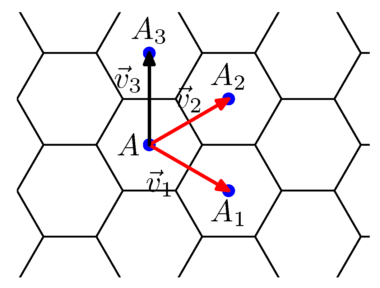
Let $M(a,b,c,d)$ be a nanotorus. As explained above, it is constructed from the infinite tiling of a plane by hexagons by cutting out the characteristic parallelogram $\mathcal{P}$ with vertices $[0,0]$, $[a,b]$, $[a+c,b+d]$, and $[c,d]$, and gluing properly opposite sides of $\mathcal{P}$. There is an alternative description of the construction of $M(a,b,c,d)$. Take again the infinite tiling of a plane by hexagons $\mathcal{H}$ with the standard basis $\overrightarrow{v_1}$ and $\overrightarrow{v_2}$ as described above (see Figure 1). For every point $T=[p,q]$, $p,q\in \mathbb{Z}$, identify T with all points $T+x(a,b)+y(c,d)=[p+xa+yc,q+xb+yd]$, where $x,y\in \mathbb{Z}$. Obviously, the resulting map is $M(a,b,c,d)$. Observe that this construction immediately implies that for every pair of hexagons A and B in $M(a,b,c,d)$, there is an automorphism of $M(a,b,c,d)$ mapping A to B. In other words, the dual of $M(a,b,c,d)$ is vertex-transitive.

Now take the infinite tiling of a plane by hexagons $\mathcal{H}$ and consider the set of points

$$S(a,b,c,d)=\left\{[xa+yc,xb+yd];x,y\in \mathbb{Z}\right\}.$$

Then $S(a,b,c,d)$ is precisely the set of points which are identified with $[0,0]$ in the construction of $M(a,b,c,d)$. We call it the mesh of points of $M(a,b,c,d)$ (see Figure 6).

Let us choose a different pair of linearly independent vectors $(a^{\prime },b^{\prime })$ and $(c^{\prime },d^{\prime })$. If $S(a,b,c,d)=S(a^{\prime },b^{\prime },c^{\prime },d^{\prime })$, then $M(a,b,c,d)$ and $M(a^{\prime },b^{\prime },c^{\prime },d^{\prime })$ are obtained by identifying the same sets of points, so they are isomorphic. Obviously, $M(a,b,c,d)$ and $M(a^{\prime },b^{\prime },c^{\prime },d^{\prime })$ are isomorphic also if there exists an automorphism of $\mathcal{H}$ which maps the set of points $S(a,b,c,d)$ to $S(a^{\prime },b^{\prime },c^{\prime },d^{\prime })$. It is interesting that the opposite implication is also true. We have the following.

Proposition 12.

Let $(a,b),(c,d)$ and $(a^{\prime },b^{\prime }),(c^{\prime },d^{\prime })$ be two pairs of linearly independent vectors. Then $M(a,b,c,d)$ and $M(a^{\prime },b^{\prime },c^{\prime },d^{\prime })$ are isomorphic if and only if there is an automorphism of $\mathcal{H}$ fixing $[0,0]$ and mapping $S(a,b,c,d)$ to $S(a^{\prime },b^{\prime },c^{\prime },d^{\prime })$.

We remark that Proposition 12 is a direct consequence of the fact that a plane regularly covers a torus. Nevertheless, our proof is elementary and shows the importance of normal cycles, see also the examples below the proof.

Proof. 

Since the sufficiency is trivial, it suffices to prove that if $M(a,b,c,d)$ and $M(a^{\prime },b^{\prime },c^{\prime },d^{\prime })$ are isomorphic nanotori, then there is an automorphism of $\mathcal{H}$ fixing $[0,0]$ and mapping $S(a,b,c,d)$ to $S(a^{\prime },b^{\prime },c^{\prime },d^{\prime })$. To simplify the notation, denote by M and $M^{\prime }$ the maps $M(a,b,c,d)$ and $M(a^{\prime },b^{\prime },c^{\prime },d^{\prime })$, respectively. In addition, denote by S and $S^{\prime }$ the sets $S(a,b,c,d)$ and $S(a^{\prime },b^{\prime },c^{\prime },d^{\prime })$, respectively. Moreover, if $[x,y]$ is a point of $\mathcal{H}$ which is a center of a hexagon, we denote by ${[x,y]}^M$ and ${[x,y]}^{M^{\prime }}$ the corresponding hexagons in M and $M^{\prime }$, respectively.

As already mentioned, three normal cycles are passing through every hexagon in M. Consider the normal cycle created by hexagons ${[0,0]}^M,{[1,0]}^M,{[2,0]}^M,\cdots$ and denote its length by n. Then, $\left({[0,1]}^M,{[1,1]}^M,\cdots ,{[n-1,1]}^M\right)$ forms another normal cycle. Since every hexagon has exactly six neighbors in M, these two cycles are either identical or disjoint. Since M is a finite map, proceeding in this way we construct several disjoint cycles of hexagons, say r, while the $(r+1)$-st cycle is identical with the first one. Consequently, $[0,0]$ is identified with $[m,r]$ for some m. We choose $m\ge 0$ to be the smallest integer such that the previous statement is satisfied.

By the definition of normal cycle, we have $[n,0]\in S$ and no internal point of the line segment starting at $[0,0]$ and terminating at $[n,0]$ is in S. Hence, S contains only the points $\left\{\right[xn,0];x\in \mathbb{Z}\}$ on the line $\{[0,0]+z\overrightarrow{v_1};z\in \mathbb{R}\}$. In addition, $[x,y]\notin S$ if $0<y<r$. But $[m,r]\in S$ and also $[m+xn,r]\in S$ for $x\in \mathbb{Z}$. Extending this argumentation to the whole plane we get

$$S=\left\{[xn+ym,yr];x,y\in \mathbb{Z}\right\}=S(n,0,m,r)$$

and M is isomorphic to $M(n,0,m,r)$. Figure 7 shows the nanotori $M(3,1,-1,3)$ and $M(10,0,3,1)$. Observe that these nanotori are isomorphic.

Now let $\phi$ be an isomorphism mapping M to $M^{\prime }$. Since the duals of nanotori are vertex transitive, we may assume that $\phi \left({[0,0]}^M\right)={[0,0]}^{M^{\prime }}$. Let $V_1$ and $V_2$ be points of $\mathcal{H}$ such that $\phi \left({[1,0]}^M\right)=V_1^{M^{\prime }}$ and $\phi \left({[0,1]}^M\right)=V_2^{M^{\prime }}$. Then for $O=[0,0]$ the vectors $\overrightarrow{O{V}_1}$ and $\overrightarrow{O{V}_2}$ both connect centers of neighboring hexagons in $\mathcal{H}$; hence, they have the same length as $\overrightarrow{v_1}$ and $\overrightarrow{v_2}$, and $O{V}_1{V}_2$ is an equilateral triangle. Thus, there is an automorphism $\psi$ of $\mathcal{H}$ fixing $[0,0]$ and mapping $\overrightarrow{v_1}$ to $\overrightarrow{O{V}_1}$ and $\overrightarrow{v_2}$ to $\overrightarrow{O{V}_2}$.

Since $\phi$ is an isomorphism, the chain of hexagons $C_0=\left(O^{M^{\prime }},{(O+\overrightarrow{O{V}_1})}^{M^{\prime }},\cdots ,{(O+(n-1)\overrightarrow{O{V}_1})}^{M^{\prime }}\right)$ is a normal cycle in $M^{\prime }$. For the very same reasons, the cycles $C_i=\left({(O+i\overrightarrow{O{V}_2})}^{M^{\prime }},{(O+\overrightarrow{O{V}_1}+i\overrightarrow{O{V}_2})}^{M^{\prime }},\cdots ,{(O+(n-1)\overrightarrow{O{V}_1}+i\overrightarrow{O{V}_2})}^{M^{\prime }}\right)$ are different from $C_0$ if $1\le i<r$, while $C_r$ is identical with $C_0$. Consequently, $M^{\prime }$ is isomorphic to $M(n,0,m^{\prime },n)$ for some $m^{\prime }$. (Observe that for this isomorphism one has to apply $\psi$.) However, $\left({[0,0]}^M,{[1,0]}^M,\cdots ,{[m,0]}^M,{[m,1]}^M,{[m,2]}^M,\cdots ,{[0,0]}^M\right)$ is a cycle of hexagons in M which “turns left” by one hexagon at ${[m,0]}^M$ and “turns right" by one hexagon at ${[0,0]}^M$. Hence, $\left(O^{M^{\prime }},{(O+\overrightarrow{O{V}_1})}^{M^{\prime }},\cdots ,{(O+m\overrightarrow{O{V}_1})}^{M^{\prime }},{(O+m\overrightarrow{O{V}_1}+\overrightarrow{O{V}_2})}^{M^{\prime }},\cdots ,{(O+\overrightarrow{O{V}_1}+(r-1)\overrightarrow{O{V}_2})}^{M^{\prime }}\right)$ must be a cycle of hexagons in $M^{\prime }$ turning by one hexagon at ${(O+m\overrightarrow{O{V}_1})}^{M^{\prime }}$ and oppositely turning by one hexagon at $O^{M^{\prime }}$ since $\phi$ is an isomorphism mapping M to $M^{\prime }$. Thus, $m=m^{\prime }$ and

$$S^{\prime }=\left\{x\left(n\overrightarrow{O{V}_1}\right)+y\left(m\overrightarrow{O{V}_1}+r\overrightarrow{O{V}_2}\right);x,y\in \mathbb{Z}\right\}.$$

Since

$$S=\left\{x\left(n\overrightarrow{v_1}\right)+y(m\overrightarrow{v_1}+r\overrightarrow{v_2});x,y\in \mathbb{Z})\right\}$$

and $\psi$ is an automorphism of $\mathcal{H}$ mapping $\overrightarrow{v_1}$ to $\overrightarrow{O{V}_1}$ and $\overrightarrow{v_2}$ to $\overrightarrow{O{V}_2}$, we get the result. □

In the next two paragraphs we consider few examples. Characteristic parallelogram for $M(3,1,-1,3)$ is given in Figure 4a. Start at $[0,0]$ and construct a normal cycle in direction of $\overrightarrow{v_1}$. This normal cycle contains all hexagons of the nanotorus, hence $r=1$; n equals the number of hexagons, i.e., $n=10$. The center $[0,0]$ is identified with $\dots ,[-7,1],[3,1],[13,1],\dots$, i.e., with $[3+nk,1]$, $k\in \mathbb{Z}$ (see Figure 7). Thus, $M(3,1,-1,3)$ is isomorphic to $M(10,0,3+10k,1)$, $k\in \mathbb{Z}$. Choosing $-n<m<n$, one obtains $M(10,0,3,1)$ and $M(10,0,-7,1)$. Recall that three normal cycles are passing through every hexagon, one in each direction $\overrightarrow{v_1}$, $\overrightarrow{v_2}$ and $\overrightarrow{v_3}$. Analogously, in the direction of $\overrightarrow{v_2}$ and $\overrightarrow{v_3}$, we find isomorphic nanotori $M(10,0,2+10k,1)$ and $M(5,0,2+5k,2)$, $k\in \mathbb{Z}$, respectively.

In Figure 4b, there is a characteristic parallelogram for $M(3,-2,-1,4)$. Start at $[0,0]$ and construct a normal cycle in direction of $\overrightarrow{v_1}$. This normal cycle does not contain all hexagons of the nanotorus, there is also another normal cycle “parallel” to it. Hence, $r=2$ and $n=5$. Figure 8 shows that $m=2$. Thus, $M(3,-2,-1,4)$ is isomorphic to $M(5,0,2+5k,2)$, $k\in \mathbb{Z}$. Plugging $k=0$, one obtains $M(5,0,2,2)$. Transitivity implies that $M(3,1,-1,3)$ and $M(3,-2,-1,4)$ are isomorphic nanotori.

In the sequel, we describe all automorphisms of $\mathcal{H}$ fixing $[0,0]$ and then we find all pairs of linearly independent vectors $(a^{\prime },b^{\prime })$ and $(c^{\prime },d^{\prime })$ such that for the meshes of points $S(a,b,s,d)=S(a^{\prime },b^{\prime },c^{\prime },d^{\prime })$.

The group of automorphisms of $\mathcal{H}$ fixing $[0,0]$ is the dihedral group $D_{12}$. It consists of 6 rotations and 6 reflections. Let $\rho$ be an anti-clockwise rotation by angle $2\pi /6={60}^{\circ }$ around $[0,0]$. Observe that $\rho$ maps $\overrightarrow{v_1}$ to $\overrightarrow{v_2}$ and $\overrightarrow{v_2}$ to $\overrightarrow{v_3}=-\overrightarrow{v_1}+\overrightarrow{v_2}$. Let $\sigma$ be a reflexion with axis $x\overrightarrow{v_1}$, where $x\in \mathbb{R}$. The elements of the group of automorphisms of $\mathcal{H}$ fixing $[0,0]$ are $\mathrm{id},\rho ,{\rho }^2,{\rho }^3,{\rho }^4,{\rho }^5,\sigma ,\sigma \rho ,\sigma {\rho }^2,\sigma {\rho }^3,\sigma {\rho }^4,\sigma {\rho }^5$, where $\mathrm{id}$ is the identity. Let $[p,q]$ be an arbitrary point of $\mathcal{H}$. We have

$$\begin{array}{cc}\mathrm{id}\left(\right[p,q\left]\right)=[p,q]\hfill & \sigma \left(\right[p,q\left]\right)=[p+q,-q]\hfill \\ \rho \left(\right[p,q\left]\right)=[-q,p+q]\hfill & \sigma \rho \left(\right[p,q\left]\right)=[q,p]\hfill \\ {\rho }^2\left([p,q]\right)=[-p-q,p]\hfill & \sigma {\rho }^2\left([p,q]\right)=[-p,p+q]\hfill \\ {\rho }^3\left([p,q]\right)=[-p,-q]\hfill & \sigma {\rho }^3\left([p,q]\right)=[-p-q,q](*)\hfill \\ {\rho }^4\left([p,q]\right)=[q,-p-q]\hfill & \sigma {\rho }^4\left([p,q]\right)=[-q,-p]\hfill \\ {\rho }^5\left([p,q]\right)=[p+q,-p]\hfill & \sigma {\rho }^5\left([p,q]\right)=[p,-p-q].\hfill \end{array}$$

Now we find all vectors $(a^{\prime },b^{\prime })$ and $(c^{\prime },d^{\prime })$ such that $S(a,b,c,d)=S^{\prime }(a^{\prime },b^{\prime },c^{\prime },d^{\prime })$. We have the following statement.

Lemma 1.

Let $(a,b),(c,d)$ and $(a^{\prime },b^{\prime }),(c^{\prime },d^{\prime })$ be two pairs of linearly independent vectors. Then, $S(a,b,c,d)=S(a^{\prime },b^{\prime },c^{\prime },d^{\prime })$ if and only if there are $x_1,y_1,x_2,y_2\in \mathbb{Z}$ such that $(a^{\prime },b^{\prime })=x_1(a,b)+y_1(c,d)$, $(c^{\prime },d^{\prime })=x_2(a,b)+y_2(c,d)$ and $|x_1{y}_2-x_2{y}_1|=1$.

Proof. 

Denote $S=S(a,b,c,d)$ and $S^{\prime }=S(a^{\prime },b^{\prime },c^{\prime },d^{\prime })$. First we show the necessity of the conditions. Hence, suppose that $S=S^{\prime }$. Since $S=\left\{[xa+yc,xb+yd];x,y\in \mathbb{Z}\right\}$, all points of $S^{\prime }$ must be of the form $[xa+yc,xb+yd]$ for some $x,y\in \mathbb{Z}$. Hence, also $(a^{\prime },b^{\prime })$ and $(c^{\prime },d^{\prime })$, the vectors determining the sides of the characteristic parallelogram for $M(a^{\prime },b^{\prime },c^{\prime },d^{\prime })$, must be of this form. So there are $x_1,y_1\in \mathbb{Z}$ such that $(a^{\prime },b^{\prime })=x_1(a,b)+y_1(c,d)$ and there are $x_2,y_2\in \mathbb{Z}$ such that $(c^{\prime },d^{\prime })=x_2(a,b)+y_2(c,d)$.

By Proposition 1, $M(a,b,c,d)$ has exactly $|ad-bc|$ hexagons while $M(a^{\prime },b^{\prime },c^{\prime },d^{\prime })$ has

$$\begin{array}{ccc}\hfill |a^{\prime }{d}^{\prime }-b^{\prime }{c}^{\prime }|& =& |(x_{1}a+y_{1}c)(x_{2}b+y_{2}d)-(x_{1}b+y_{1}d)(x_{2}a+y_{2}c)|\hfill \\ & =& |(x_1{x}_2-x_1{x}_2)ab+(x_1{y}_2-x_2{y}_1)ad+(x_2{y}_1-x_1{y}_2)bc+(y_1{y}_2-y_1{y}_2)cd|\hfill \\ & =& |x_1{y}_2-x_2{y}_1|·|ad-bc|\hfill \end{array}$$

of them. Thus, $|x_1{y}_2-x_2{y}_1|=1$.

On the other hand, suppose that there are $x_1,y_1,x_2,y_2\in \mathbb{Z}$ such that $\left(a^{\prime }{b}^{\prime }\right)=x_1(a,b)+y_1(c,d)$, $(c^{\prime },d^{\prime })=x_2(a,b)+y_2(c,d)$ and $|x_1{y}_2-x_2{y}_1|=1$. Obviously $S^{\prime }\subseteq S$ since every point of $S^{\prime }$ has the form

$$\begin{array}{ccc}\hfill x[a^{\prime },b^{\prime }]+y[c^{\prime },d^{\prime }]& =& x{x}_1[a,b]+x{y}_1[c,d]+y{x}_2[a,b]+y{y}_2[c,d]=\hfill \\ & =& [(x{x}_1+y{x}_2)a+(x{y}_1+y{y}_2)c,(x{x}_1+y{x}_2)b+(x{y}_1+y{y}_2)d]=\hfill \\ & =& [\tilde{x}a+\tilde{y}c,\tilde{x}b+\tilde{y}d]=\tilde{x}[a,b]+\tilde{y}[c,d]\hfill \end{array}$$

for some $x,y\in \mathbb{Z}$, where $\tilde{x}=x{x}_1+y{x}_2$ and $\tilde{y}=x{y}_1+y{y}_2$. It suffices to show that $S\subseteq S^{\prime }$. However, we have

$$\left(\begin{array}{cccc}{x}_1& 0& y_1& 0\\ 0& x_1& 0& y_1\\ x_2& 0& y_2& 0\\ 0& x_2& 0& y_2\end{array}\right)\left(\begin{array}{c}a\\ b\\ c\\ d\end{array}\right)=\left(\begin{array}{c}{a}^{\prime }\\ b^{\prime }\\ c^{\prime }\\ d^{\prime }\end{array}\right).$$

(1)

If we denote the matrix by $\mathbb{A}$, then (1) states that $\mathbb{A}·{(a,b,c,d)}^T={(a^{\prime },b^{\prime },c^{\prime },d^{\prime })}^T$. Since $\left|\mathbb{A}\right|={(x_1{y}_2-x_2{y}_1)}^2=1$, we get

$${\mathbb{A}}^{-1}=\left(\begin{array}{cccc}{x}_1{y}_2^2-x_2{y}_1{y}_2& 0& x_2{y}_1^2-x_1{y}_1{y}_2& 0\\ 0& x_1{y}_2^2-x_2{y}_1{y}_2& 0& x_2{y}_1^2-x_1{y}_1{y}_2\\ x_2^2{y}_1-x_1{x}_2{y}_2& 0& x_1^2{y}_2-x_1{x}_2{y}_1& 0\\ 0& x_2^2{y}_1-x_1{x}_2{y}_2& 0& x_1^2{y}_2-x_1{x}_2{y}_1\end{array}\right).$$

Since ${(a,b,c,d)}^T={\mathbb{A}}^{-1}·{(a^{\prime },b^{\prime },c^{\prime },d^{\prime })}^T$, for $x_1^{\prime }=x_1{y}_2^2-x_2{y}_1{y}_2$, $y_1^{\prime }=x_2{y}_1^2-x_1{y}_1{y}_2$, $x_2^{\prime }=x_2^2{y}_1-x_1{x}_2{y}_2$, and $y_2^{\prime }=x_1^2{y}_2-x_1{x}_2{y}_1$ we get $(a,b)=x_1^{\prime }(a^{\prime },b^{\prime })+y_1^{\prime }(c^{\prime },d^{\prime })$ and $(c,d)=x_2^{\prime }(a^{\prime },b^{\prime })+y_2^{\prime }(c^{\prime },d^{\prime })$, which implies that $S\subseteq S^{\prime }$. □

Combining Proposition 12 and Lemma 1, we get the following statement.

Theorem 2.

Let $(a,b),(c,d)$ and $(a^{\prime },b^{\prime }),(c^{\prime },d^{\prime })$ be two linearly independent pairs of vectors. Then the nanotori $M(a,b,c,d)$ and $M(a^{\prime },b^{\prime },c^{\prime },d^{\prime })$ are isomorphic if and only if there are $x_1,y_1,x_2,y_2\in \mathbb{Z}$, and an automorphism of $\mathcal{H}$ fixing $[0,0]$ and mapping $(a,b)$ to $(a^{*},b^{*})$ and $(c,d)$ to $(c^{*},d^{*})$ such that $(a^{\prime },b^{\prime })=x_1(a^{*},b^{*})+y_1(c^{*},d^{*})$, $(c^{\prime },d^{\prime })=x_2(a^{*},b^{*})+y_2(c^{*},d^{*})$ and $|x_1{y}_2-x_2{y}_1|=1$.

Or equivalently, by taking (*) into account, we have

Theorem 3.

Let $(a,b),(c,d)$ and $(a^{\prime },b^{\prime }),(c^{\prime },d^{\prime })$ be two pairs of linearly independent vectors. Then the nanotori $M(a,b,c,d)$ and $M(a^{\prime },b^{\prime },c^{\prime },d^{\prime })$ are isomorphic if and only if there are $x_1,y_1,x_2,y_2\in \mathbb{Z}$ such that $|x_1{y}_2-x_2{y}_1|=1$ and at least one of the following holds

 1:

$(a^{\prime },b^{\prime })=x_1(a,b)+y_1(c,d)$ and $(c^{\prime },d^{\prime })=x_2(a,b)+y_2(c,d)$;

 2:

$(a^{\prime },b^{\prime })=x_1(-b,a+b)+y_1(-d,c+d)$ and $(c^{\prime },d^{\prime })=x_2(-b,a+b)+y_2(-d,c+d)$;

 3:

$(a^{\prime },b^{\prime })=x_1(-a-b,a)+y_1(-c-d,c)$ and $(c^{\prime },d^{\prime })=x_2(-a-b,a)+y_2(-c-d,c)$;

 4:

$(a^{\prime },b^{\prime })=x_1(a+b,-b)+y_1(c+d,-d)$ and $(c^{\prime },d^{\prime })=x_2(a+b,-b)+y_2(c+d,-d)$;

 5:

$(a^{\prime },b^{\prime })=x_1(b,a)+y_1(d,c)$ and $(c^{\prime },d^{\prime })=x_2(b,a)+y_2(d,c)$;

 6:

$(a^{\prime },b^{\prime })=x_1(-a,a+b)+y_1(-c,c+d)$ and $(c^{\prime },d^{\prime })=x_2(-a,a+b)+y_2(-c,c+d)$.

Theorem 3 (2) and (3) imply that $M(3,1,-1,3)$, $M(-1,4,-3,2)$, and $M(4,-1,2,-3)$ are isomorphic nanotori, see Figure 9. Observe that the equation $|x_1{y}_2-x_2{y}_1|=1$ has infinitely many solutions in $\mathbb{Z}$. This fact together with Theorems 2 and 3 imply the following.

Corollary 1.

Each torus $M(a,b,c,d)$ is isomorphic to infinitely many tori $M(a^{\prime },b^{\prime },c^{\prime },d^{\prime })$.

Redundancy of the Parameters of $M(a,b,c,d)$

Hence, the last corollary motivates us to look for quadruples having 0 as one of the four parameters. Indeed, we find n, r, and m, such that $M(a,b,c,d)$ is isomorphic to $M(n,0,m,r)$. In what follows, we treat general nanotorus $M(a,b,c,d)$ and naturally we assume that $(a,b)$ and $(c,d)$ are linearly independent vectors.

Corollary 2.

Let x and y be integer solutions of the equation $xb+yd=\mathrm{GCD}(b,d)$. Then, $M(a,b,c,d)$ is isomorphic to $M(n,0,m,r)$, where $r=\mathrm{GCD}(b,d)$, $n=|ad-bc|/r$ and $m\equiv xa+yc(modn)$.

Proof. 

Observe that b and d cannot be both equal to 0 since $(a,b)$ and $(c,d)$ are linearly independent. Without loss of generality we assume that $d\ne 0$. Choose $x_1=\frac{d}{\mathrm{GCD}(b,d)}\frac{ad-bc}{|ad-bc|}$ and $y_1=\frac{-b}{\mathrm{GCD}(b,d)}\frac{ad-bc}{|ad-bc|}$.

Then

$$x_1(a,b)+y_1(c,d)=\left(\frac{(ad-bc)}{\mathrm{GCD}(b,d)}\frac{(ad-bc)}{|ad-bc|},0\right)=\left(\frac{|ad-bc|}{r},0\right)=(n,0).$$

Let $x_2$ and $y_2$ be integer solutions of equation $x_{2}b+y_{2}d=\mathrm{GCD}(b,d)$. Then, for $m^{\prime }=x_{2}a+y_{2}c$ we get

$$x_2(a,b)+y_2(c,d)=(m^{\prime },r).$$

Since $y_2=\left(\mathrm{GCD}(b,d)-x_{2}b\right)/d$, we get

$$|x_1{y}_2-x_2{y}_1|=|\frac{d}{\mathrm{GCD}(b,d)}\frac{ad-bc}{|ad-bc|}\frac{\mathrm{GCD}(b,d)-x_{2}b}{d}-x_2\frac{-b}{\mathrm{GCD}(b,d)}\frac{ad-bc}{|ad-bc|}|=1.$$

Thus, $M(a,b,c,d)$ is isomorphic to $M(n,0,m^{\prime },r)$, by Theorem 3 (1). Since $M(n,0,m^{\prime },r)$ is isomorphic to $M(n,0,m^{\prime }+zn,r)$ for arbitrary $z\in \mathbb{Z}$ by Theorem 3 (1), we get the result. □

By Theorem 3 (2), $M(a,b,c,d)$ is isomorphic to $M(-b,a+b,-d,c+d)$, and by Theorem 3 (3), $M(a,b,c,d)$ is isomorphic to also to $M(-a-b,a,-c-d,c)$. The parallelograms for $M(-b,a+b,-d,c+d)$ and $M(-a-b,a,-c-d,c)$ are obtained from the parallelogram for $M(a,b,c,d)$ by $\rho$ and ${\rho }^2$, respectively. Recall that three normal cycles are passing through every hexagon of $M(a,b,c,d)$. One normal cycle in $M(a,b,c,d)$ is $({[0,0]}^M,{[1,0]}^m,\dots )$, i.e., moving in the direction of $\overrightarrow{v_1}$. The other two are moving in directions of $\overrightarrow{v_2}$ and $\overrightarrow{v_3}$, respectively. The alternative way to obtain the other two normal cycles in $M(a,b,c,d)$ is to move in direction of $\overrightarrow{v_1}$ in $M(-b,a+b,-d,c+d)$ and $M(-a-b,a,-c-d,c)$, respectively. Thus, we can generalize Corollary 2 to the following result.

Corollary 3.

Let $s=|ad-bc|$, $r_1=\mathrm{GCD}(b,d)$, $r_2=\mathrm{GCD}(a+b,c+d)$ and $r_3=\mathrm{GCD}(a,c)$. Denote $n_i=s/r_i$ for $1\le i\le 3$, and

• $m_1\equiv x_{1}a+y_{1}c(mod{n}_1)$, where $x_1,y_1$ are integer solutions of $x_{1}b+y_{1}d=r_1$;
• $m_2\equiv -x_{2}b-y_{2}d(mod{n}_2)$, where $x_2,y_2$ are integer solutions of $x_2(a+b)+y_2(c+d)=r_2$;
• $m_3\equiv x_3(-a-b)+y_3(-c-d)(mod{n}_3)$, where $x_3,y_3$ are integer solutions of $x_{3}a+y_{3}c=r_3$.

Then $M(a,b,c,d)$ is isomorphic to $M(n_i,0,m_i,r_i)$ for every i, $1\le i\le 3$.

As mentioned above, through every hexagon of $M(a,b,c,d)$ three normal cycles are passing and, by Corollary 3, their lengths are $n_1$, $n_2$, and $n_3$. Hence, this corollary gives us the possibility to represent $M(a,b,c,d)$ with one side of the characteristic parallelogram being the vector $(n,0)$, where n is the length of the longest normal cycle in the nanotorus, and there are infinitely many such representations In addition, the vector $(m,r)$, the second side of the parallelogram, can be chosen such that $m<n$.

Applying Corollary 3 to $M(3,1,-1,3)$, we find that it is isomorphic to $M(10,0,3,1)$, $M(10,0,-7,1)$, $M(10,0,2,1)$, $M(10,0,-8,1)$, $M(5,0,2,2)$, $M(5,0,-3,2)$, and infinitely many others. In this case $r_1=r_3=1$ and $r_2=2$. If Corollary 3 is applied to $M(4,0,0,4)$, $r_1=r_2=r_3=4$, $n_1=n_2=n_3=4$, and respectively $m_1=m_2=m_3$. Hence, the nanotori $M(4,0,-8,4)$, $M(4,0,-4,4)$, $M(4,0,8,4)$, $M(4,0,12,4)$, and infinitely many others are isomorphic to $M(4,0,0,4)$.

Proposition 6 and Corollary 3 imply the following.

Corollary 4.

The nanotorus $M(a,b,c,d)$ is isomorphic to $M^{*}(r_i,n_i,{(m_i+r_i)}_n)$ where $n_i,m_i,r_i$ for $1\le i\le 3$ are determined in Corollary 3.

Similarly, Proposition 9 and Corollary 3 imply the relation between the nanotorus $M(a,b,c,d)$ and generalized honeycomb tori $\mathrm{GHT}$.

Corollary 5.

The nanotorus $M(a,b,c,d)$ is isomorphic to the generalized honeycomb torus $\mathrm{GHT}(r_i,2n_i,c_i)$ where $c_i={(2m_i+r_i)}_{2n_i}$ and $n_i,m_i,r_i$ for $1\le i\le 3$ are determined in Corollary 3.

Applying Corollary 4 to $M(3,1,-1,3)$, we find that this nanotorus is isomorphic to $M^{*}(1,10,3)$, $M^{*}(1,10,4)$, $M^{*}(1,10,7)$, $M^{*}(1,10,8)$, $M^{*}(2,5,3)$, and $M^{*}(2,5,4)$. Analogously, by Corollary 5, one can find six different triplets $(a_i,b_i,c_i)$, $1\le i\le 6$ such that $\mathrm{GHT}(a_i,b_i,c_i)$ is isomorphic to $M(3,1,-1,3)$. They are $\mathrm{GHT}(1,20,7)$, $\mathrm{GHT}(1,20,5)$, $\mathrm{GHT}(1,20,13)$, $\mathrm{GHT}(1,20,5)$, $\mathrm{GHT}(2,10,4)$, and $\mathrm{GHT}(2,10,6)$. It is worth mentioning that there are cases, such as $M(4,0,0,4)$, that have only one representation with respect to Altshuler, $M^{*}(4,4,0)$, or as generalized honeycomb torus, $\mathrm{GHT}(4,4,0)$. From these remarks it is obvious that a given nanotorus might have one or more (at most six) different Altshuler (resp. generalized honeycomb torus) representations. For more details, refer to the counting of the representations we refer to [27,28].

5. Concluding Remarks

We studied three, known in the literature, approaches for constructing nanotori. The first one was suggested by Altshuler. Later, inspired by by real life problems, two new and different approaches were introduced; one for describing nanotori molecules, and another one for describing interconnecting networks in computer science. In his work Altshuler showed that his method gives all non-isomorphic nanotori, but for the last two definitions there were no such results. Here we showed that the later two approaches also construct all nanotori. At the same time, we gave explicit formulas that convert parameters of one construction into the parameters of the other two constructions. The equivalence of these three constructions can be used for evaluating different graph measures as topological indices.

The four parameters construction is mainly used in chemistry and physics to describe carbon nanotori molecules. We show that there are infinitely many quadruples that determine the same nanotorus, and we characterize when two different quadruples define isomorphic nanotori. Even more, we gave an explicit form of all isomorphic nanotori (defined with four parameters). This result significantly narrows the realm of search of the molecule with desired properties.

References

1. Iijima, S. Helical microtubules of graphitic carbon. Nature 1991, 354, 56–58. [Google Scholar] [CrossRef]
2. Dunlap, B.I. Connecting carbon tubules. Phys. Rev. B 1992, 46, 1933–1936. [Google Scholar] [CrossRef] [PubMed]
3. Liu, J.; Dai, H.; Hafner, J.H.; Colbert, D.T.; Smalley, R.E.; Tans, S.J.; Dekker, C. Fullerene “Crop circles”. Nature 1997, 385, 780–781. [Google Scholar] [CrossRef]
4. Martel, R.; Shea, H.R.; Avouris, P. Ring formation in single-wall carbon nanotubes. J. Phys. Chem. B 1999, 103, 7551–7556. [Google Scholar] [CrossRef]
5. Haddon, R. Electronic properties of carbon toroids. Nature 1997, 388, 31–32. [Google Scholar] [CrossRef]
6. Lin, M.F.; Chuu, D.S. Persistent currents in toroidal carbon nanotubes. Phys. Rev. B 1998, 57, 6731–6737. [Google Scholar] [CrossRef]
7. Liu, L.; Guo, G.Y.; Jayanthi, C.S.; Wu, S.Y. Colossal Paramagnetic Moments in Metallic Carbon Nanotori. Phys. Rev. Lett. 2001, 88, 217206–217210. [Google Scholar] [CrossRef] [Green Version]
8. Sarapat, P.; Hill, J.M.; Baowan, D. A Review of Geometry, Construction and Modelling for Carbon Nanotori. Appl. Sci. 2019, 9, 2301. [Google Scholar] [CrossRef] [Green Version]
9. Tsai, C.C.; Shyu, L.F.; Chiu, C.W.; Chang, C.P.; Chen, B.R.; Lin, M.F. Magnetization of armchair carbon tori. Phys. Rev. B 2004, 70, 075411. [Google Scholar] [CrossRef]
10. Liu, L.; Liu, F.; Zhao, J. Curved carbon nanotubes: From unique geometries to novel properties and peculiar applications. Nano Res. 2014, 7, 626–657. [Google Scholar] [CrossRef]
11. Andova, V.; Knor, M.; Škrekovski, R. Distances on nanotubical graphs. J. Math. Chem. 2016, 54, 1575–1584. [Google Scholar] [CrossRef]
12. Andova, V.; Knor, M.; Škrekovski, R. Distances based indices on nanotubical graphs: Part 1. J. Math. Chem. 2018, 56, 2801–2815. [Google Scholar] [CrossRef]
13. Andova, V.; Knor, M.; Škrekovski, R. Distances based indices on nanotubical graphs: Part 2. J. Math. Chem. 2018, 56, 3076–3088. [Google Scholar] [CrossRef]
14. Arezoomand, M.; Taeri, B. The full symmetry and irreducible representations of nanotori. Acta Crystallogr. A 2009, 65, 249–252. [Google Scholar] [CrossRef]
15. Dienes, K.R.; Thomas, B. Isospectral But Physically Distinct: Modular Symmetries and their Implications for Carbon Nanotori. Phys. Rev. B 2011, 84, 085444. [Google Scholar] [CrossRef] [Green Version]
16. Zhang, Z.; Yang, Z.; Wand, X.; Yuan, J.H.; Zhang, M.Q. The electronic structure of a deformed chiral carbon nanotorus. J. Phys. Condens. Matter 2005, 17, 249–255. [Google Scholar] [CrossRef]
17. Damnjanović, M.; Vuković, T.; Milošević, I.; Nikolić, B. Symmetry of single-wall nanotubes. Acta Cristal. A 2001, 57, 304–310. [Google Scholar] [CrossRef] [Green Version]
18. Staic, M.D.; Petresku-Nita, A. Symmetry group of two special types of carbon nanotori. Acta Cristal. A 2013, 69, 435–439. [Google Scholar] [CrossRef]
19. Yavari, M.; Ashrafi, A.R. On the Symmetry of a Zig-Zag and an Armchair Polyhex Carbon Nanotorus. Symmetry 2009, 1, 145–152. [Google Scholar] [CrossRef]
20. Zurawski, R. Embedded Systems Handbook: Embedded Systems Design and Verification; CRC Press: San Francisco, CA, USA, 2018. [Google Scholar]
21. Cho, H.; Hsu, L. Generalized honeycomb torus. Inf. Process. Lett. 2003, 86, 185–190. [Google Scholar] [CrossRef]
22. Megson, G.M.; Yang, X.; Liu, X. Honeycomb tori are Hamiltonian. Inf. Process. Lett. 1999, 72, 99–103. [Google Scholar] [CrossRef]
23. Stojmenović, I. Honeycomb networks: Topological properties and communication Algorithms. IEEE Trans. Parallel Distrib. Syst. 1997, 8, 1036–1042. [Google Scholar] [CrossRef] [Green Version]
24. Shih, Y.-K.; Wu, Y.-C.; Kao, S.-S.; Tana, J.J.M. Vertex-bipancyclicity of the generalized honeycomb tori. Comp. Math. Appl. 2008, 56, 2848–2860. [Google Scholar] [CrossRef] [Green Version]
25. Altshuler, A. Hamiltonian circuits in some maps on the torus. Discret. Math. 1972, 1, 299–314. [Google Scholar] [CrossRef] [Green Version]
26. Altshuler, A. Construction and enumeration of regular maps on the torus. Discret. Math. 1973, 4, 201–217. [Google Scholar] [CrossRef] [Green Version]
27. Brehma, U.; Kühnel, W. Equivelar maps on the torus. Eur. J. Combin. 2008, 29, 1843–1861. [Google Scholar] [CrossRef] [Green Version]
28. Hubard, I.; Orbanić, A.; Pellicer, D.; Ivić Weiss, A. Symmetries of Equivelar 4-Toroids. Discret. Comput. Geom. 2012, 48, 1110–1136. [Google Scholar] [CrossRef] [Green Version]
Figure 1. Standard basis of the hexagonal tiling.
Mathematics 08 02036 g001
Figure 2. Characteristic parallelogram for M ( 3 , 1 , 1 , 3 ) .
Mathematics 08 02036 g002
Figure 3. Construction of a nanotorus M * ( 3 , 4 , 1 ) . Points A, B * , and E * coincide. Blue segments form a hexagon on M * ( 3 , 4 , 1 ) .
Mathematics 08 02036 g003
Figure 4. (a) Normal cycle in M ( 3 , 1 , 1 , 3 ) , r = 1 . (b) Normal cycles in M ( 3 , 2 , 1 , 4 ) , r = 2 . The characteristic parallelogram for M ( 3 , 2 , 1 , 4 ) is obtained by rotation of the characteristic parallelogram M ( 3 , 1 , 1 , 3 ) for 60 .
Mathematics 08 02036 g004
Figure 5. Generalized honeycomb torus GHT ( 3 , 8 , 7 ) .
Mathematics 08 02036 g005
Figure 6. A mesh of points of M ( 3 , 1 , 1 , 3 ) , i.e., S ( 3 , 1 , 1 , 3 ) .
Mathematics 08 02036 g006
Figure 7. Characteristic parallelogram (gray) for M ( 3 , 1 , 1 , 3 ) and characteristic parallelogram (green) for M ( 10 , 0 , 3 , 1 ) . The nanotori they define are isomorphic.
Mathematics 08 02036 g007
Figure 8. Characteristic parallelogram (gray) for M ( 3 , 2 , 1 , 4 ) and characteristic parallelogram (green) for M ( 5 , 0 , 2 , 2 ) . These parallelograms define isomorphic nanotori.
Mathematics 08 02036 g008
Figure 9. The gray parallelogram, A B C D is defining M ( 3 , 1 , 1 , 3 ) nanotori. The green parallelogram A B C D , in (a) is obtained by reflection and in (b) by rotation. (a) ρ ( M ( 3 , 1 , 1 , 3 ) ) = M ( 1 , 4 , 3 , 2 ) ; (b) σ ( M ( 3 , 1 , 1 , 3 ) ) = M ( 4 , 1 , 2 , 3 ) .
Mathematics 08 02036 g009
Publisher’s Note: MDPI stays neutral with regard to jurisdictional claims in published maps and institutional affiliations.