1. Introduction
Stroke and spinal cord injury are the main causes of disability in the elderly [
1,
2], creating problems in daily life. For many years, rehabilitation therapies have been concentrated on recovering their motion function using various manual methods. In recent years, the lower-limb exoskeleton, which is a wearable robot, has been used to aid patients with mobility problems [
3,
4,
5].
For the exoskeleton wearer to walk properly, the desired trajectory of the joints requires a robust control system to minimize steady-state errors to reduce disturbances. Huo et al. [
6] proposed an active impedance control strategy for controlling a lower-limb exoskeleton for the sit-to-stand motion. Many researchers focused on adaptive-based control approaches to design a controller with uncertainties and non-linear systems. For instance, Daachi et al. [
7] controlled one degree of freedom (DoF) lower-limb knee joint orthosis using a neural network based on adaptive control using the Lyapunov approach for rehabilitation reasons. Chen et al. [
8] studied an adaptive robust cascade force control for a one DoF exoskeleton with a hydraulic actuator to minimize the effect of uncertainties. Lu et al. [
9] described an adaptive learning control system with unknown parameters using the Lyapunov approach for stability. In another study, Yang et al. [
10] designed a robust learning controller with hybrid electro-hydraulic actuators, and verified their exoskeleton using a periodic reference.
For many years, proportional-integral-derivative (PID) controllers have been commonly used because of their reliable performance, and convenient and robust operation [
11,
12,
13]. In our approach, we used particle swarm optimization (PSO) to tune the PID controller’s gains. PSO has a simple concept and is easy to implement in different optimization problems. Hence, it has been used to control the robustness of PID parameters [
14]. PSO has few parameters that need to be adjusted, and it has high probability and efficiency in finding the global optima, but initializing its parameters can be difficult. Although PSO has fast error convergence, it can converge prematurely and be trapped in the local optima [
15]. Therefore, researchers have combined different tuning methods to optimize its gains. For example, Belkadi et al. [
16] developed an optimal method to obtain the parameters of the PID controller and verified the performance in a simulation using PSO with random initialization. Similarly, Durgadevi et al. [
17] used PSO for tuning the parameters of proportional-integral (PI) and PID controllers of the temperature of a continuous stirred tank reactor.
As an alternative to PSO, other optimization methods have been used for tuning controller parameters [
18]. Qianhao et al. [
19] developed the whale optimization algorithm, which is a type of swarm intelligence optimization algorithm, to improve the performance of a linear–quadratic regulator controller. Pan et al. [
20] presented the fuzzy-PID algorithm for the nonlinear dynamics and uncertainties of the human exoskeleton robot. Their method was verified in a co-simulation technique combining ADAMS and MATLAB/Simulink. Moharam et al. [
21] used a hybrid differential evolution and PSO algorithm for tuning a PID controller and compared it with the genetic algorithm (GA) and the Ziegler–Nichols (Z-N) method to prove the hybrid method is robust to disturbances. Lal et al. [
22] implemented the grasshopper optimization algorithm (GOA) to obtain the PID and fuzzy-PID controller parameters for a multi-area interconnected microgrid power system. They compared two different PID controllers and concluded that fuzzy-PID produced better dynamic responses compared to a PID controller tuned by GOA.
This paper presents the tuning of PID controller gains by combining Z-N and adaptive particle swarm optimization (APSO). A simulation and the dynamic equation of the human exoskeleton model walking with the aid of a parallel bar in a virtual environment are described. The transfer functions of each joint based on the dynamic equation of human exoskeleton model are established in a closed-loop control system. An objective function formulated by the error of the control system is defined. Our main objective was to optimize a PID controller using initialization with Z-N and optimized by APSO. The tuned PID was verified in the 3-dimensional virtual simulation environment and compared with the conventional method.
2. Human Exoskeleton Simulation in a Virtual Environment
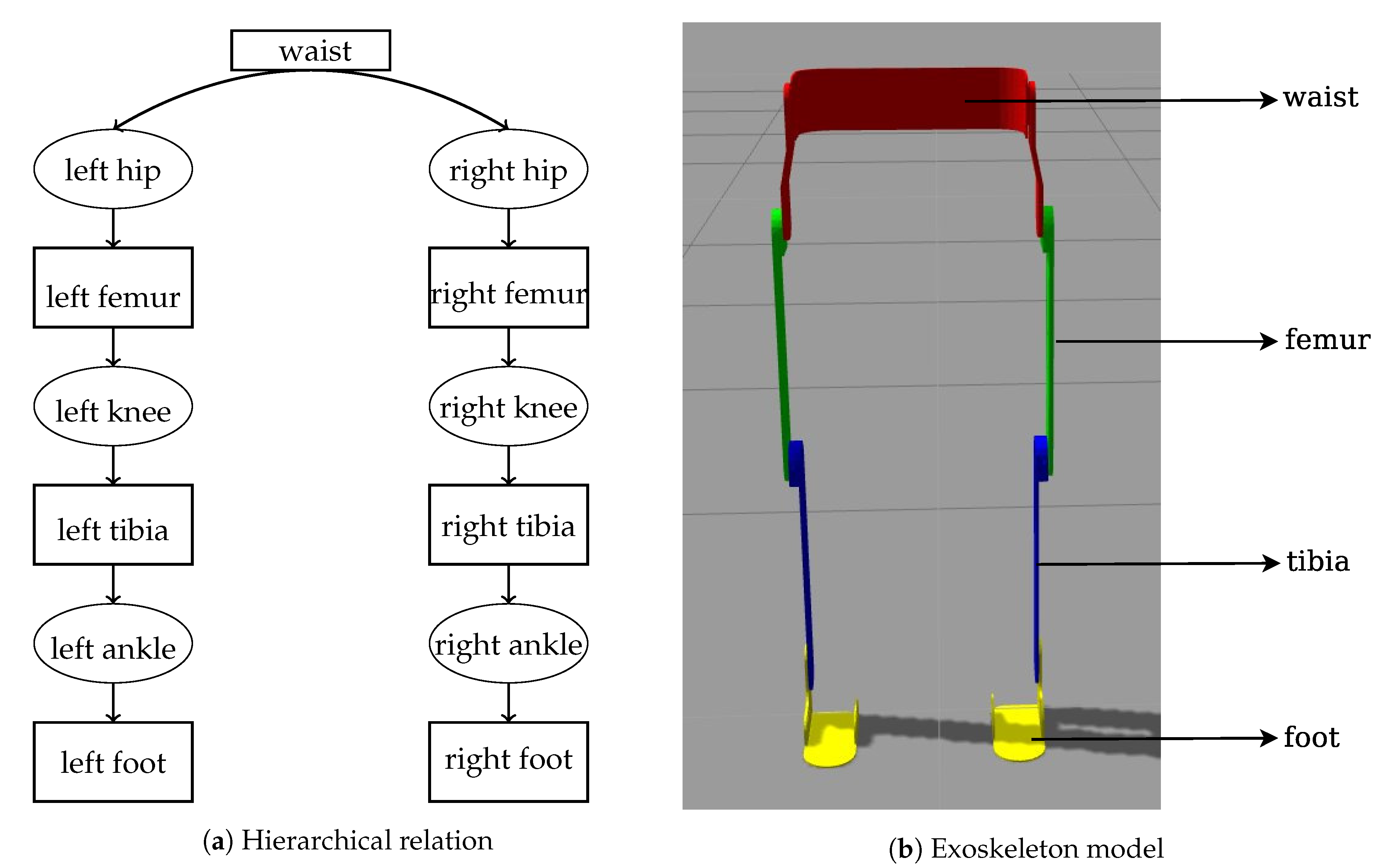
The lower-limb exoskeleton model consists of a waist, left and right femurs, left and right tibias, and left and right feet. The human exoskeleton simulated model was created and controlled in a robot operating system (ROS) with average human anthropometric height. The waist functions as a base link to which the left and right femurs are connected. Consequently, other links are assembled to each other as parent and child links [
23].
Figure 1a,b shows the hierarchical relation of the 3D exoskeleton model in an open-source dynamic simulator that imitates the behavior in a real environment.
To simulate the interaction between the exoskeleton and patient, a 3D human model was added in the Gazebo simulation environment. The foot, tibia, and femur of human are coupled to its related links. The configurations of coupling between human and exoskeleton model are shown in
Figure 2.
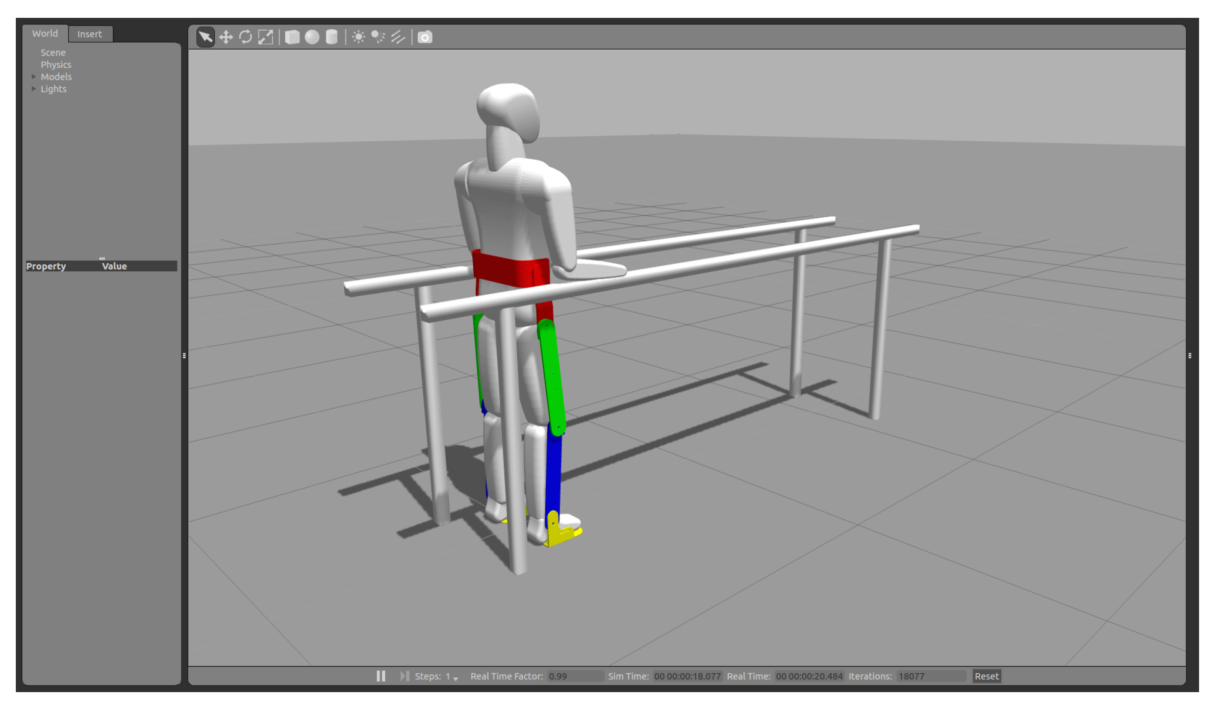
To ensure the simulation accurately mimicked to the gait training task, parallel bars were added to avoid the human model from falling down by providing stability. Both hands of the human model are constrained to the parallel bars using a slide joint to allow forward and backward motion.
Figure 3 demonstrates the gait training simulation of the human exoskeleton model walking with both hands holding the parallel bars.
3. Human Exoskeleton Dynamic Modeling
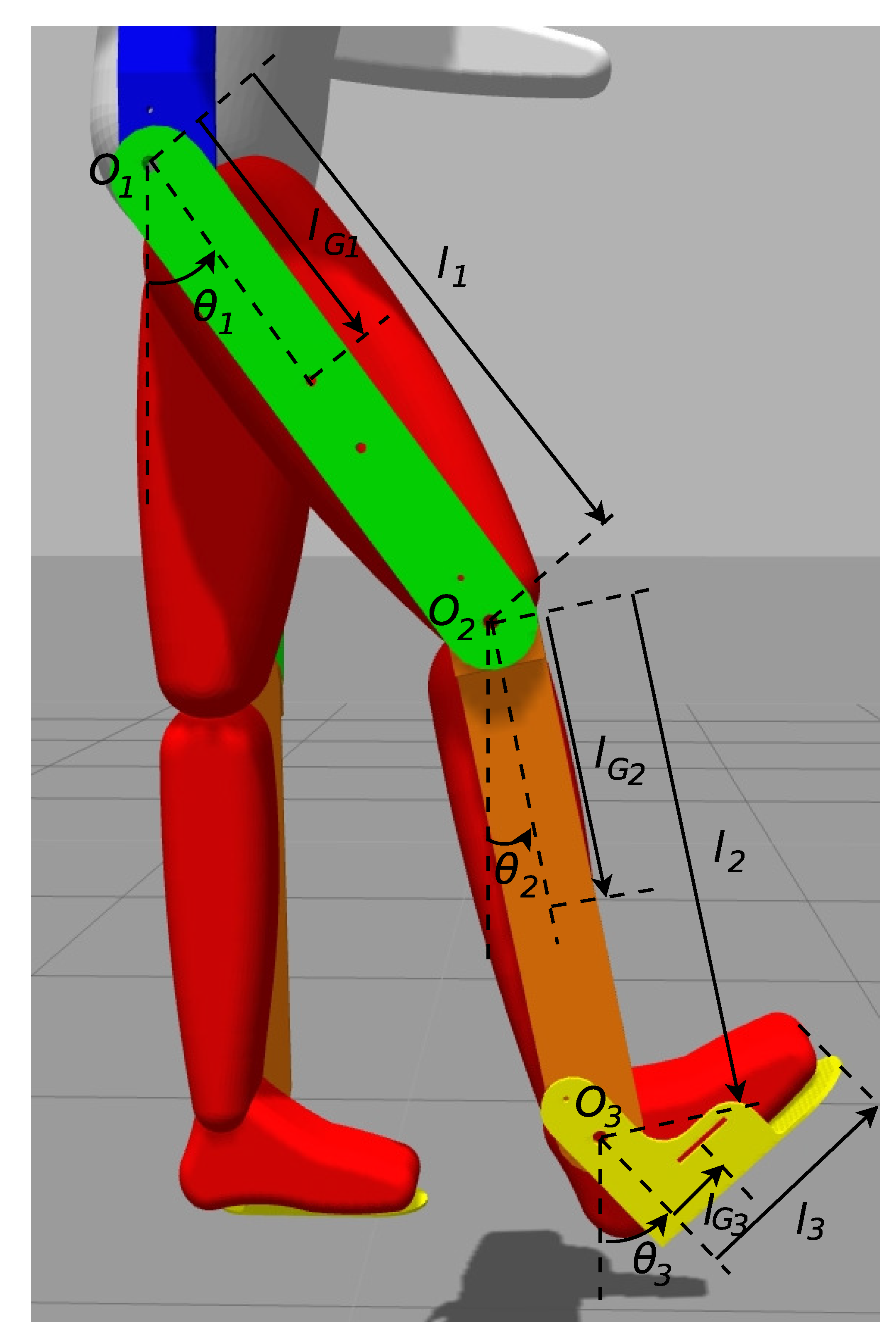
Figure 4 illustrates a free body diagram of the exoskeleton and human model.
,
, and
are the center position of hip, knee, and ankle joint, respectively;
,
, and
represent angles of hip, knee, and ankle, respectively;
,
, and
are length of the femur, tibia, and foot, respectively; and
is the center of gravity (CoG) of links 1, 2, and 3.
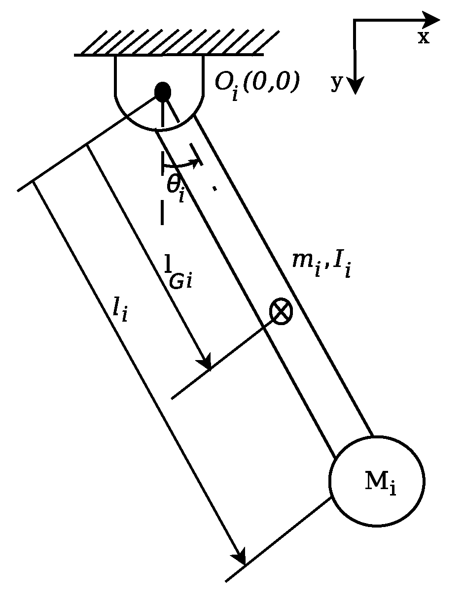
In this paper, each link of the exoskeleton and human is modeled as one DoF pendulum model, which replicates one joint of the exoskeleton and human, as shown in
Figure 5. The summation of the physical effect of each lower link such as mass and inertia is considered to be
[
24].
In this study, the Lagrangian formulation of dynamic equation of the pendulum model is expressed as follows:
where
i represents number of the links;
is the Lagrangian function;
and
are the angular position and velocity, respectively;
is the torque that applies to each joint; and
and
represent kinetic and potential energy [
25], respectively, which are given as follows:
where
and
are the mass and inertia of the link, respectively;
is the mass of lower links;
g represents gravitational acceleration;
,
,
,
,
, and
, represent the position of the CoG, end point of the link, and their velocity, respectively, as follows:
where
and
are the length of the CoG and the link
i, respectively. The total kinetic and potential energies are determined as follows:
The dynamic equation of the pendulum model is determined as follows:
where
b is the friction coefficient and
is approximated as
. The transfer function
is represented in Laplace as follows:
Table 1 lists the physical features of the exoskeleton based on computer-automated design (CAD). The human model’s features were obtained from References [
26,
27,
28]. The mass and inertia of the human model were for a subject that weighed 74.2 kg and was 175.5 cm tall.
Based on the features, the transfer function of the exoskeleton (
) and human (
) can be determined as shown in
Table 2.
5. Optimization of the Controller’s Gains
The PID controller is tuned using an algorithm by a combination of the Z-N method and APSO. The PID parameters are obtained from Z-N, which is the classical observation method of tuning [
31]. The output is set as the initial value, which provides the searching space to avoid local optima [
32]. APSO increases the speed of convergence and the chance of finding the global optimum. PSO is based on population, inspired from observation of biological social phenomena such as a flock of birds, swarms of bees, and schools of birds [
33].
An objective function
of the optimization problem is defined as the integral time absolute error (ITAE), which is the summation of the absolute error weighted by the elapsed time [
34,
35], as follows:
where the error of control system is given as follows:
where
t is the elapsed time;
and
represent the error of the control system in the time and frequency domains, respectively. The tuning algorithm starts with Z-N, where
and
are set to zero while the
value is established as
. The value of
is added until the first oscillation is observed, then its frequency is calculated as
. The gains of the PID are determined as follows:
where
is the output that is input into APSO, which contains particles as design variables for minimizing the objective function. Initialization is created by randomizing
as follows:
where
represents the particles in the first iteration;
is a positive value, which is selected as a random value between 0 and 1.
The particles of the next iteration are a summation of the positions of previous particles with their velocities:
where
k and
j represent the numbers of iterations and particles, respectively;
and
are the position of the current particle and the particle of the previous iteration, respectively; and
is the velocity and direction of each particle toward the next iteration as follows:
where
and
are random values between 0 and 1;
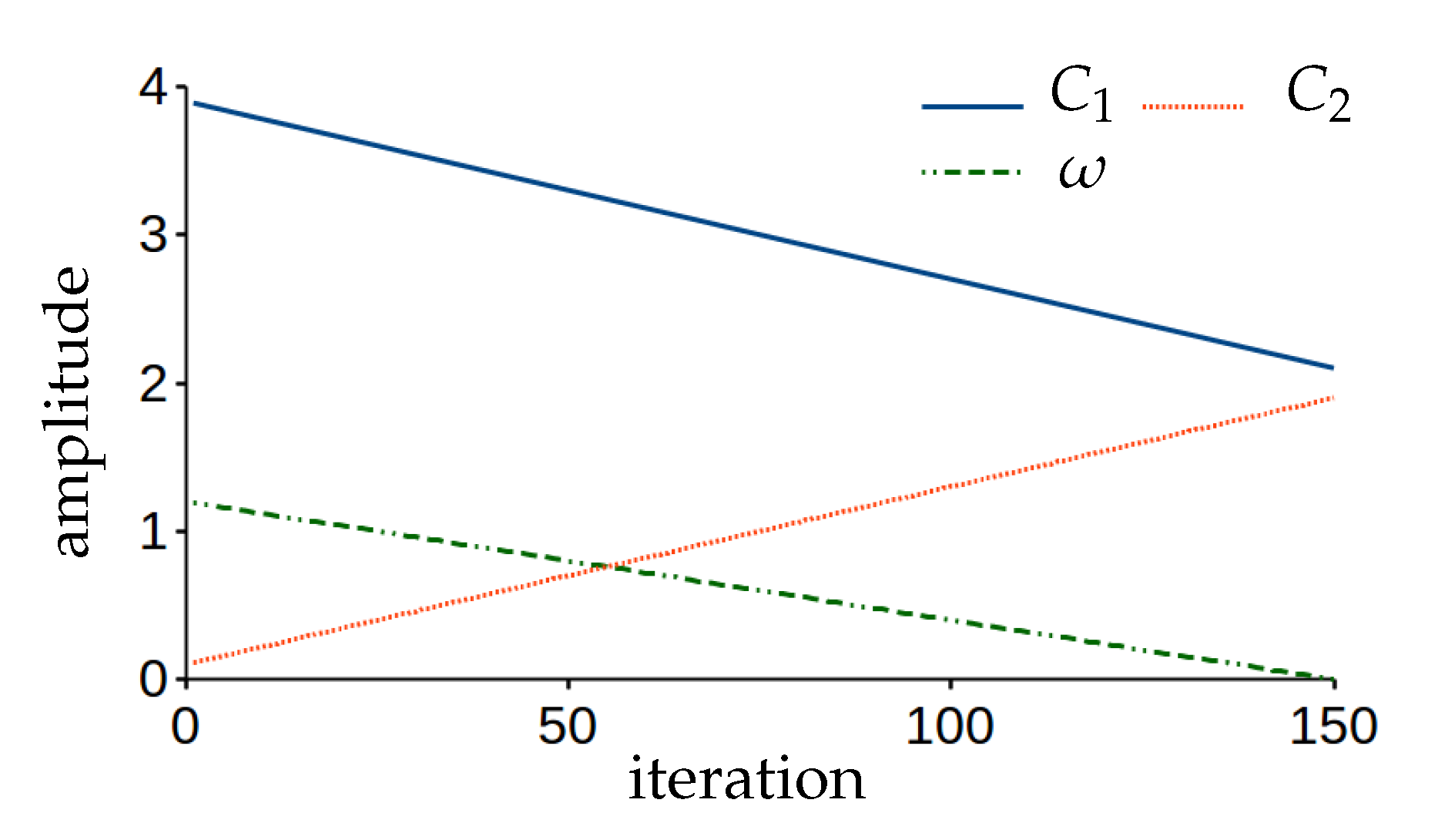
is a positive coefficient, called inertia weight, which reduces linearly with iteration, and is determined as follows:
where
is the maximum value for inertia weight;
b is a gain that starts from 1 in the first iteration and end to 0, which allows
starts from the maximum value to have wider searching space and decrease to be narrowed toward the global optima [
36]; and
b is a positive descending coefficient, starting from 1 in the first iteration.
b is represented as follows:
where
a is a positive ascending coefficient, which starts from 0 and increases to 1 at the last iteration, as follows:
where
k and
are the maximum number of iterations;
and
are non-negative coefficients of self and social recognition, defined as follows:
The value of
is greater than
, and their summation remains at 4 in all iterations [
36]. In each iteration, the objective function is determined for each particle, and the smallest objective function is selected as
. The value of
will be the lowest value of
when the algorithm ends. ASPO stops when the number of iterations meets the maximum number of iterations
. In this paper, the numbers of iterations and particles are 150 and 30, respectively, which were determined by experimentation to obtain the convergence of the objective function values to zero. Algorithm 1 and
Figure 7 illustrate the pseudo code and flow chart of the APSO algorithm, respectively, where
is a constant value for a step of
.
| Algorithm 1 Combination of Ziegler–Nichols (Z-N) and adaptive particle swarm optimization (APSO). |
- 1:
Start - 2:
- 3:
Set ; - 4:
- 5:
Set ; - 6:
- 7:
Set ; - 8:
- 9:
Initialize ; - 10:
- 11:
Set step value for - 12:
- 13:
while Observe oscillation do; - 14:
- 15:
Set ; - 16:
- 17:
; - 18:
- 19:
end while - 20:
- 21:
Calculate frequency of the oscillation as ; - 22:
- 23:
Calculate , , and - 24:
- 25:
Initialize population around the output of Z-N results; - 26:
- 27:
Evaluate initial population; - 28:
- 29:
Selecting the initial ; - 30:
- 31:
while Number of iteration less than do; - 32:
- 33:
Create new iteration; - 34:
- 35:
Select the ; - 36:
- 37:
if less than the previous then; - 38:
- 39:
Store it as - 40:
- 41:
end if - 42:
- 43:
end while - 44:
- 45:
Select the particle of as the result - 46:
- 47:
End
|
Figure 8 shows the
in each iteration for three joints of the human exoskeleton.
The changes in
and
for 150 iterations are shown in
Figure 9 and the
in each iteration.
Table 3 demonstrates the optimal gains of the PID controller.
6. Results and Discussion
The desired trajectory of each joint is based on gait training to move the joints simultaneously. The trajectories of each joint are driven by two different functions, repeated periodically.
Table 4 shows the desired trajectory.
t represents the elapsed time and
is the time of one walking cycle.
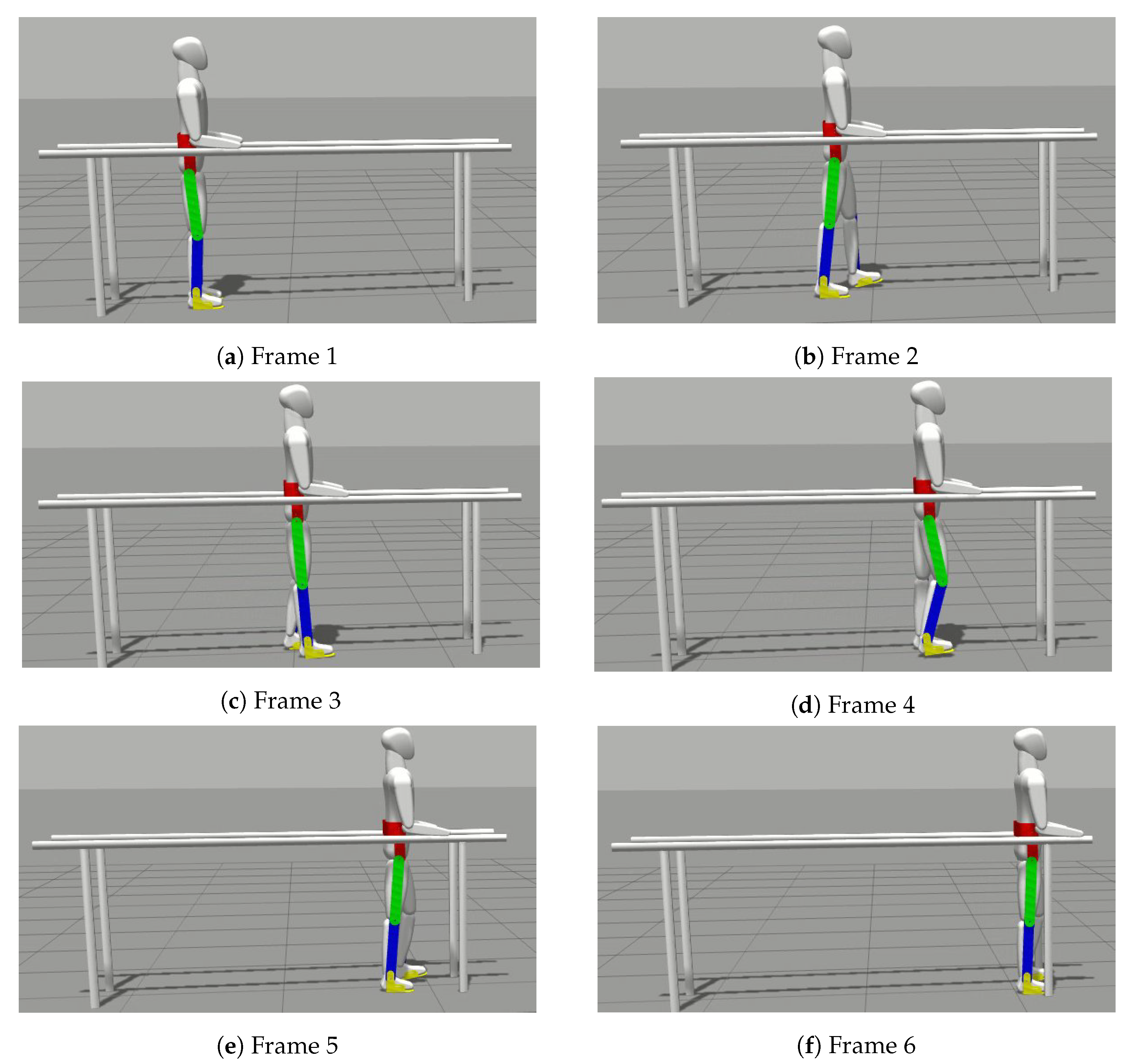
Figure 10 provides the frame-by-frame pictures of gait training with parallel bars.
The APSO algorithm was coded in Python programming language, and the virtual environment was Gazebo, integrated with ROS. All tests were performed using a PC with a Ubuntu 18.04 LTS operation system with 16 GB RAM and an Intel core-i3 Xeon processor.
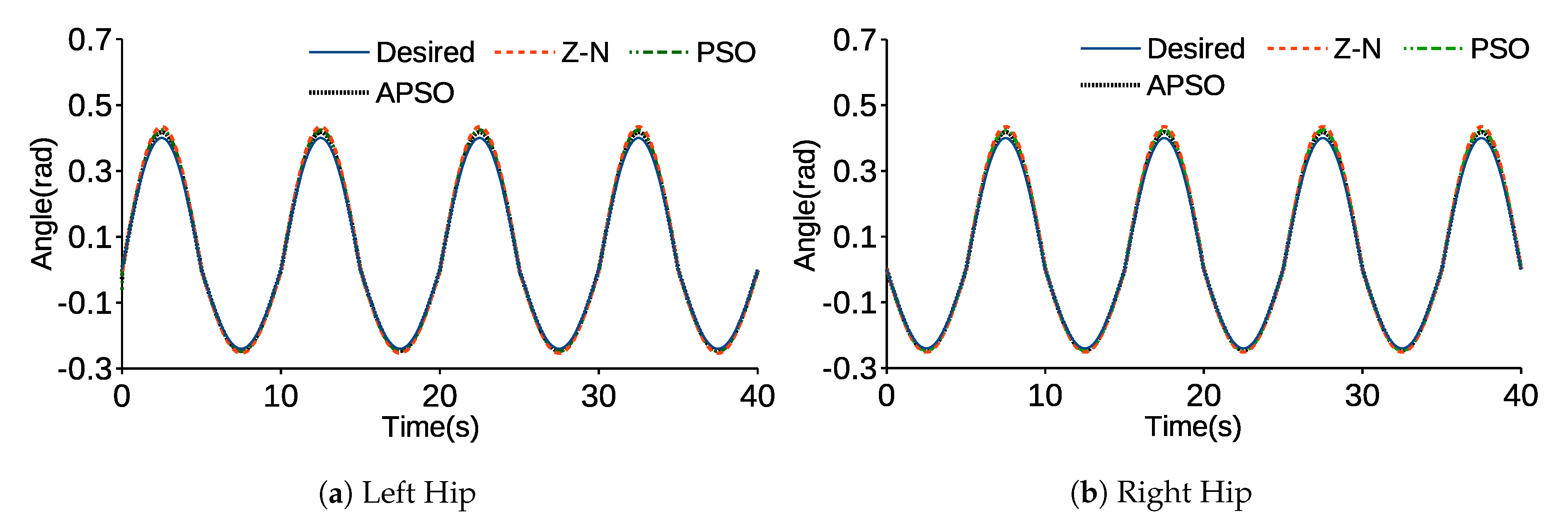
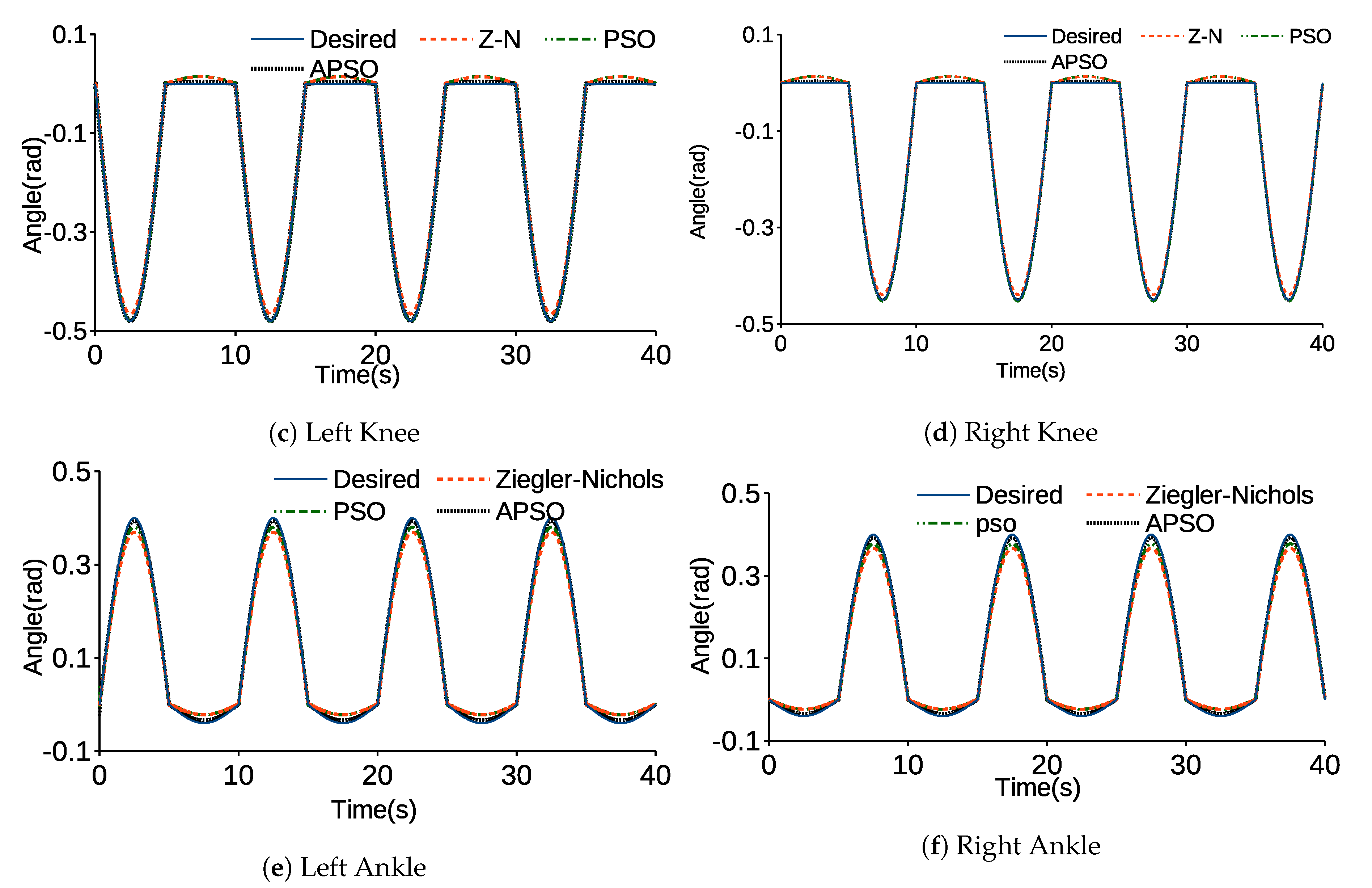
Figure 11 exhibits the performance of the simulated model in Gazebo. The graphs compare the trajectories of Z-N, PSO, and APSO with the desired trajectory. The Z-N measured the initial values for PSO and APSO. The difference between PSO and APSO is the method of setting the parameters. In PSO,
,
, and
are adjusted to 1.2, 2, and 2, respectively.
Figure 12 shows the angular error trajectory for the hip, knee, and ankle. For all joints, the APSO error was the lowest, followed by PSO and Z-N. For example, the average error determined by APSO for the hip was 24% and 48% is less than PSO and Z-N, respectively. APSO showed less overshoot than the other methods because of its smaller peak, whereas PSO and Z-N experienced more shock when the trajectory changed.
Figure 13 demonstrates the output torque of each link. The maximum torques of the knee and ankle were less than 3 and 0.05 Nm, respectively. The maximum amplitude of torque for the hip was 7 Nm, which is the highest because the actuator of the hip tolerates a heavier mass compared to the knee and ankle.
Table 5 provides the numerical analysis of Z-N and APSO performance.
,
,
, and
represent the maximum error, average error, root mean square error, and coefficient of determination, respectively. The maxima of
and
were less than 0.03 m, which are within the acceptable zone [
37]. The maximum of
was 0.0130, while the
values of all joints were greater than 99%, indicating the close fitted of all variability in the actual trajectories.
7. Conclusions
In this study, a PID controller was optimally tuned using an optimization algorithm that combines of Z-N and APSO. Parameter changes in each iteration enabled the finding of the optimal solution and avoided the local optima. Furthermore, the PID gains were established by Z-N and used for initializing the APSO. The proposed method was compared and tested in a virtual environment on a human exoskeleton model. The results demonstrated the acceptable performance of the APSO controller by statistical analysis.
The optimal PID controller minimized the trajectory error of a multi-joint human exoskeleton structure for gait training. For a new trajectory and different training conditions, the optimization process should be repeated, which is the limitation of this study. In future work, the model can be applied in different situations such as climbing stairs and the stand-to-sit movement.

 ,
, 


