An Integral Equation Approach to the Irreversible Investment Problem with a Finite Horizon

Abstract

This paper studies an irreversible investment problem under a finite horizon. The firm expands its production capacity in irreversible investments by purchasing capital to increase productivity. This problem is a singular stochastic control problem and its associated Hamilton–Jacobi–Bellman equation is derived. By using a Mellin transform, we obtain the integral equation satisfied by the free boundary of this investment problem. Furthermore, we solve the integral equation numerically using the recursive integration method and present the graph for the free boundary.

1. Introduction

In economics, optimal investment problems have received much attention over the last few decades. In particular, optimal investment problems under uncertainty have been widely studied with the mathematical approaches. Abel and Eberly [1] provided an explicit analytic function for optimal investment under the uncertainty of a firm with costly reversibility. To formulate the investment problem, a constant-return-to-scale Cobb–Douglas production function facing an isoelastic demand curve was considered over infinite time. Eberly and Mieghem [2] showed an optimal investment strategy in a non-stationary case with uncertainty, a concave profit function and a horizon of arbitrary length. Bertola [3] studied an irreversible investment problem under uncertainty with an infinite horizon. In [3], the problem was solved under Cobb–Douglas technology and constant elasticity demand. Dangl [4] investigated an irreversible investment problem when a firm decides on optimal investment timing and optimal capacity choice at the same time under the condition of uncertainty demand. In this paper, we deal with an irreversible investment problem under uncertainty. More specifically, the main contribution of this paper is an efficient derivation of the integral equation for an irreversible investment problem using Mellin transforms.

We consider an optimal irreversible investment problem under uncertainty with a finite horizon. Specifically, we employ the partial differential equation (PDE) approach to solve the problem and derive the integral equation for the free boundary of the investment problem using Mellin transforms. The important advantage of Mellin transforms is that they convert the given PDE into the simple ordinary differential equation (ODE). This leads to closed-form or analytic solutions of the PDEs. Thus, Mellin transforms have been used widely as a relevant tool to handle the PDE in the financial area. In recent years, the diverse options have been studied with Mellin transforms by many researchers (cf. [5,6,7,8,9]). In particular, pricing formulas for vulnerable options under the structural model have been derived using the double Mellin transforms (cf. [10,11,12,13,14,15]). We also adopt a Mellin transform approach to derive the integral equation for irreversible optimal investment with a finite horizon. The properties of double Mellin transforms are used appropriately to obtain the integral equation for the optimal investment with a finite horizon. This approach induces the integral equation more efficiently.

The remainder of this paper is organized as follows. Section 2 presents a brief literature review on optimal investment problems. In Section 3, we formulate the model for the irreversible investment problem with the production function. In Section 4, we deal with the free boundary problem for the irreversible optimal investment. Concretely, the integral equation for the free boundary (the investment threshold) to maximize firm value is derived by using Mellin transforms. We give the concluding remarks in Section 5.

2. Literature Review

Optimal investment problems have been developed by many researchers. Chiarolla and Haussmann [16] studied an irreversible investment problem in a stochastic, continuous time model over a finite time and obtained the free boundary for optimal stopping problem from a nonlinear integral. Ewald and Wang [17] dealt with an irreversible investment problem under the Cox–Ingersoll–Ross (CIR) model. They showed various advantages of the CIR model. Riedel and Su [18] studied a sequential irreversible investment problem under uncertainty and provided a general approach for irreversible investment problems. Chiarolla, Ferrari and Riedel [19] dealt with a stochastic irreversible investment problem in a market with N firms. Chiarolla and Ferrari [20] and Ferrari [21] also found a new integral equation for the free boundaries of irreversible investment problems on finite and infinite time horizons, respectively. In addition, Ferrari and Salminen [22] studied a general irreversible investment problem under Lévy uncertainty as a two-dimensional, degenerate, singular stochastic control problem. De Angelis, Federico and Ferrari [23] investigated a Markovian model for optimal irreversible investment when a firm aims at minimizing total expected costs of production. More recently, Christensen and Salminen [24] proposed the Riesz representation approach for the efficient study of multidimensional investment problems. Federico, Rosestolato and Tacconi [25] dealt with a model of irreversible investment choices. They characterized an optimal stochastic impulse control problem with an infinite time horizon using techniques of viscosity. Jeon and Kim [26] considered an investment problem with partial reversibility. They derived the coupled integral equations for the optimal investment and solved the equations numerically.

3. The Model

In this paper, we assume that a firm chooses a dynamic capacity expansion plan over a finite horizon $T>0$. The firm decides on irreversible investments to expand its production capacity to achieve better productivity and its instantaneous profit is given by a constant elasticity function $\Pi (X,K)$ of

$$\begin{array}{c}\hfill \Pi (X_t,K_t)=X_t{K}_t^{\gamma },0<\gamma <1,\end{array}$$

(1)

where ${\left(X_s\right)}_{s=t}^T$ is the per-unit profit margin of the output and ${\left(K_s\right)}_{s=t}^T$ is the firm’s capital stock process. We model the firm’s output function as Q given by

$$Q_t=K_t^{\gamma }{L}_t^{1-\gamma }=K_t^{\gamma },$$

where we consider the case in which the labor L is constant over time ( $L\equiv 1$).

The dynamics of the per-unit profit margin ${\left(X_s\right)}_{s=t}^T$ are governed by geometric Brownian motion

$$\begin{array}{c}\hfill d{X}_s=\mu X_{s}ds+\sigma X_{s}d{W}_s,X_s>0,\end{array}$$

(2)

where $\mu$ and $\sigma$ are positive constants; ${\left(W_t\right)}_{t=0}^T$ is some standard Brownian motion on a complete probability space $(\Omega ,\mathcal{F},\mathbb{P})$ equipped with a filtration ${\left({\mathcal{F}}_t\right)}_{t\ge 0}$ satisfying the usual conditions.

Within the present model, the firm’s capital stock process $\left\{K_s\right\}$ evolves according to

$$\begin{array}{c}\hfill d{K}_s=d{L}_s-\delta K_{s}ds,\end{array}$$

(3)

where $\delta \ge 0$ is a depreciation rate of the firm’s capital stock and $\left(L_s\right)$ represents the cumulative purchase of capital until time $s\in [t,T]$, which is right-continuous with the left limit, nonnegative and non-decreasing for $\mathcal{F}$-adapted stochastic process with $L_{t-}=0$.

An irreversible investment policy ${\left(L_s\right)}_{s=t}^T$ is called admissible if

$$\begin{array}{c}\hfill \mathbb{E}\left[{\int }_t^T{e}^{-\beta (s-t)}(X_{s}ds+d{L}_s)\right]<+\infty .\end{array}$$

(4)

We denote by ${\mathcal{A}}_t(x,k)$ with $X_t=x{K}_t=k$ the class of all admissible policies.

The firm’s objective is to maximize the following expected utility by choosing the irreversible investment plan ${\left(L_s\right)}_{s=t}^T$:

$$\begin{array}{c}\hfill V(t,x,k)=\underset{L\in {\mathcal{A}}_t}{sup}\mathbb{E}\left[{\int }_t^T{e}^{-\beta (s-t)}\left(\Pi (X_s,K_s)ds-pd{L}_s\right)\mid X_t=x,K_t=k\right],\end{array}$$

(5)

on region $\mathcal{R}=\left\{\right(t,x,k)\mid 0\le t\le T,0<x,k<+\infty \}$, where $\beta >0$ is a discount factor.

4. Free Boundary Problem

Following Fleming and Soner [27], the associated Hamilton–Jacobi–Bellman (HJB) equation of (5) is given by

$$\begin{array}{c}\hfill min\{-{\partial }_{t}V-\mathcal{L}V-\Pi ,p-{\partial }_{k}V\}=0,V(T,x,k)=0,\end{array}$$

(6)

with

$$\mathcal{L}={\displaystyle \frac{{\sigma }^2}{2}}{x}^2{\partial }_{xx}+\mu x{\partial }_x-\delta k{\partial }_k-\beta .$$

From the HJB Equation (6), we can define the investment region and the no-investment region as follows.

$$\begin{array}{c}\hfill \begin{array}{cc}\hfill \mathbf{IR}& =\{(t,x,k)\mid {\partial }_{k}V(t,x,k)=p\},(\mathrm{the} \mathrm{investment} \mathrm{region}),\hfill \\ \hfill \mathbf{NR}& =\{(t,x,k)\mid {\partial }_{k}V(t,x,k)<p\},(\mathrm{the} \mathrm{no}-\mathrm{investment} \mathrm{region}).\hfill \end{array}\end{array}$$

(7)

Then, the boundary that separates $\mathbf{IR}$ from $\mathbf{NR}$ is referred to as the free boundary, or optimal investment threshold, and is given by

$$\begin{array}{c}\hfill B(t,k)=sup\{x\in {\mathbb{R}}_{+}\mid (t,x,k)\in \mathbf{NR}\}.\end{array}$$

(8)

The investment region and the no-investment region correspond to $x\ge B(t,k)$ and $x<B(t,k)$, respectively. In terms of the free boundary $B(t,k)$, the investment region IR can be written as

$$\begin{array}{c}\hfill \mathbf{IR}=\left\{\right(t,x,k)\mid x\ge B(t,k\left)\right\}.\end{array}$$

Moreover, at the free boundary $x=B(t,k)$, the following smooth-pasting condition is established:

$$\begin{array}{c}\hfill {\partial }_{k}V(t,B(t,k),k)=p\mathrm{and}{\partial }_{xk}V(t,B(t,k),k)=0.\end{array}$$

(9)

As in [28], we consider the following substitution

$$z={\displaystyle \frac{x^m}{k}},u(t,z)=V(t,x,k)/k,$$

where $m=1/(1-\gamma )$.

Under above substitution, the HJB Equation (6) can be reduced to one-dimensional HJB equation

$$\begin{array}{c}\hfill min\{-{\partial }_{t}u-{\mathcal{L}}^{\star }u-{\Pi }^{\star },p-(u-z{\partial }_{z}u)\}=0,u(T,z)=0,\end{array}$$

(10)

where

$$\begin{array}{c}\hfill \begin{array}{cc}\hfill \hat{\mu }& =\mu m+m(m-1){\sigma }^2/2,\hfill \\ \hfill {\mathcal{L}}^{\star }& ={\displaystyle \frac{{\sigma }^2{m}^2}{2}}{z}^2{\partial }_{zz}+(\hat{\mu }+\delta )z{\partial }_z-(\beta +\delta )\mathrm{and}{\Pi }^{\star }\left(z\right)=z^{1-\gamma }.\hfill \end{array}\end{array}$$

(11)

In terms of the value function $u(t,z)$, the investment region $\widetilde{\mathbf{IR}}$ and the no-investment region $\widetilde{\mathbf{NR}}$ are defined by

$$\begin{array}{c}\hfill \begin{array}{cc}\hfill \widetilde{\mathbf{IR}}=& \{(t,z)\mid u(t,z)-{\partial }_{z}u(t,z)=p\}\hfill \\ \hfill =& \{(t,z)\mid 0\le t<T,z\ge B^{\star }\left(t\right)\},\hfill \end{array}\end{array}$$

and

$$\begin{array}{c}\hfill \begin{array}{cc}\hfill \widetilde{\mathbf{NR}}=& \{(t,z)\mid u(t,z)-{\partial }_{z}u(t,z)<p\}\hfill \\ \hfill =& \{(t,z)\mid 0\le t<T,z<B^{\star }\left(t\right)\},\hfill \end{array}\end{array}$$

respectively.

Here, the free boundary $B^{\star }\left(t\right)$ is given by

$$B^{\star }\left(t\right)={\displaystyle \frac{B{(t,k)}^m}{k}}.$$

Let us define the function $H(t,z)$ as

$$H(t,z)\equiv u(t,z)-z{\partial }_{z}u(t,z).$$

In investment region $\widetilde{\mathbf{IR}}$,

$$H(t,z)=p.$$

In no-investment region $\widetilde{\mathbf{NR}}$, since

$${\partial }_{t}u+{\mathcal{L}}^{\star }u+z^{1-\gamma }=0,$$

It is easy to check that

$${\partial }_{t}H+{\mathcal{L}}^{\star }H+\gamma z^{1-\gamma }=0.$$

Thus, $H(t,z)$ satisfies the following non-homogeneous PDE.

$$\begin{array}{c}\hfill \begin{array}{cc}\hfill & {\partial }_{t}H+{\mathcal{L}}^{\star }H+\gamma z^{1-\gamma }{\mathbf{1}}_{\{z<B^{\star }\left(t\right)\}}+p(\beta +\delta ){\mathbf{1}}_{\{z\ge B^{\star }\left(t\right)\}}=0,\hfill \\ & H(T,z)=0.\hfill \end{array}\end{array}$$

(12)

with the smooth-pasting condition $H(t,B^{\star }\left(t\right))=p$.

Proposition 1.

The value function $H(t,z)$ can be expressed by

$$\begin{array}{c}\hfill \begin{array}{cc}\hfill H(t,z)=& p(\beta +\delta ){\int }_t^T{e}^{-M_1(\eta -t)}\mathcal{N}\left({\displaystyle \frac{log\frac{z}{B^{\star }\left(\eta \right)}+(\hat{\mu }+\delta -\frac{1}{2}{\sigma }^2{m}^2)(\eta -t)}{\sigma m\sqrt{\eta -t}}}\right)d\eta \hfill \\ & +\gamma z^{1-\gamma }{\int }_t^T{e}^{-M_2(\eta -t)}\mathcal{N}\left(-{\displaystyle \frac{log\frac{z}{B^{\star }\left(\eta \right)}+(\beta +\delta -\gamma {\sigma }^2{m}^2+\frac{1}{2}{\sigma }^2{m}^2)(\eta -t)}{\sigma m\sqrt{\eta -t}}}\right)d\eta ,\hfill \end{array}\end{array}$$

(13)

and the free boundary $B^{\star }\left(t\right)$ satisfies the following integral equation:

$$\begin{array}{c}\hfill \begin{array}{cc}\hfill p=& p(\beta +\delta ){\int }_t^T{e}^{-M_1(\eta -t)}\mathcal{N}\left({\displaystyle \frac{log\frac{B^{\star }\left(t\right)}{B^{\star }\left(\eta \right)}+(\hat{\mu }+\delta -\frac{1}{2}{\sigma }^2{m}^2)(\eta -t)}{\sigma m\sqrt{\eta -t}}}\right)d\eta \hfill \\ & +\gamma {\left(B^{\star }\left(t\right)\right)}^{1-\gamma }{\int }_t^T{e}^{-M_2(\eta -t)}\mathcal{N}\left(-{\displaystyle \frac{log\frac{B^{\star }\left(t\right)}{B^{\star }\left(\eta \right)}+(\beta +\delta -\gamma {\sigma }^2{m}^2+\frac{1}{2}{\sigma }^2{m}^2)(\eta -t)}{\sigma m\sqrt{\eta -t}}}\right)d\eta ,\hfill \end{array}\end{array}$$

(14)

where $\mathcal{N}(·)$ is standard normal cumulative distribution function and the constants $M_1$ and $M_2$ are defined by

$$\begin{array}{c}\hfill \begin{array}{c}\hfill M_1=\beta +\delta ,M_2=\beta +\delta -(1-\gamma )(\hat{\mu }+\delta -\frac{1}{2}{\sigma }^2{m}^2)-\frac{1}{2}{(1-\gamma )}^2{\sigma }^2{m}^2.\end{array}\end{array}$$

Proof. 

Let us define

$$f(t,z)=\gamma z^{1-\gamma }{\mathbf{1}}_{\{z<B^{\star }\left(t\right)\}}+p(\beta +\delta ){\mathbf{1}}_{\{z\ge B^{\star }\left(t\right)\}}.$$

Then, from the PDE (12), we have

$$\begin{array}{c}\hfill \begin{array}{cc}\hfill & {\partial }_{t}H+{\mathcal{L}}^{\star }H=-f(t,z),\hfill \\ & H(T,z)=0.\hfill \end{array}\end{array}$$

(15)

Let us consider the Mellin transform $\hat{H}(t,w)$ of $H(t,z)$; then

$$\hat{H}(t,w)={\int }_0^{\infty }H(t,z)z^{w-1}dz.$$

By the inverse Mellin transform,

$$\begin{array}{c}\hfill \begin{array}{c}\hfill H(t,z)={\displaystyle \frac{1}{2\pi i}}{\int }_{c-i\infty }^{c+i\infty }\hat{H}(t,w)z^{-w}dw.\end{array}\end{array}$$

(16)

From (16) and (15), the PDE (15) can be represented by

$$\begin{array}{c}\hfill \begin{array}{cc}\hfill & {\displaystyle \frac{d\hat{H}}{dt}}+{\displaystyle \frac{{\sigma }^2{m}^2}{2}}\mathcal{Q}\left(w\right)\hat{H}=\hat{f}(t,w),\hfill \\ & \mathcal{Q}\left(w\right)=w^2+(1-k_2)w-k_1,and{k}_1=\frac{2(\beta +\delta )}{{\sigma }^2{m}^2},k_2=\frac{2(\hat{\mu }+\delta )}{{\sigma }^2{m}^2},\hfill \end{array}\end{array}$$

(17)

where the terminal condition is $\hat{H}(T,z)=0$ and $\hat{f}(t,w)$ is the Mellin transform of $f(t,z)$.

Then, we can obtain the solution for the non-homogeneous ODE (17) as

$$\begin{array}{c}\hfill \hat{H}(t,w)={\int }_t^T{e}^{\frac{{\sigma }^2{m}^2}{2}\mathcal{Q}\left(w\right)(\eta -t)}\hat{f}(\eta ,w)d\eta .\end{array}$$

(18)

Hence, from (16),

$$\begin{array}{c}\hfill \begin{array}{c}\hfill H(t,z)={\displaystyle \frac{1}{2\pi i}}{\int }_{c-i\infty }^{c+i\infty }{\int }_t^T{e}^{\frac{{\sigma }^2{m}^2}{2}\mathcal{Q}\left(w\right)(\eta -t)}\hat{f}(\eta ,w)z^{-w}d\eta dw.\end{array}\end{array}$$

(19)

Meanwhile, if we define

$$\begin{array}{c}\hfill \begin{array}{c}\hfill \mathcal{G}(t,z):={\displaystyle \frac{1}{2\pi i}}{\int }_{c-i\infty }^{c+\infty }{e}^{\frac{{\sigma }^2{m}^2}{2}\mathcal{Q}\left(w\right)t}{z}^{-w}dw,\end{array}\end{array}$$

(20)

then from Lemma 1 in [6], $\mathcal{G}(t,z)$ leads to

$$\begin{array}{c}\hfill \begin{array}{c}\hfill \mathcal{G}(t,z)=e^{-\frac{{\sigma }^2{m}^2}{2}\{{\left(\frac{1-k_2}{2}\right)}^2+k_1\}t}{\displaystyle \frac{z^{\frac{1-k_1}{2}}}{\sigma m\sqrt{2\pi t}}}{e}^{-\frac{1}{2}{(logz/\left(\sigma m\sqrt{t}\right))}^2}.\end{array}\end{array}$$

(21)

Since $e^{\frac{{\sigma }^2{m}^2}{2}\mathcal{Q}\left(w\right)(\eta -t)}$ and $\hat{f}(\eta ,w)$ are the Mellin transforms of $\mathcal{G}(\eta -t,z)$ and $f(\eta ,z)$, by the Mellin convolution property in [6], $H(t,z)$ yields

$$\begin{array}{c}\hfill \begin{array}{cc}\hfill H(t,z)=& {\int }_t^T{\int }_0^{\infty }f(\eta ,u)\mathcal{G}(\eta -t,{\displaystyle \frac{z}{u}}){\displaystyle \frac{du}{u}}d\eta \hfill \\ \hfill =& {\int }_t^T{\int }_{B^{\star }\left(\eta \right)}^{\infty }p(\beta +\delta )\mathcal{G}(\eta -t,{\displaystyle \frac{z}{u}}){\displaystyle \frac{du}{u}}d\eta +\gamma {\int }_t^T{\int }_0^{B^{\star }\left(\eta \right)}{u}^{1-\gamma }\mathcal{G}(\eta -t,{\displaystyle \frac{z}{u}}){\displaystyle \frac{du}{u}}d\eta .\hfill \end{array}\end{array}$$

(22)

By Appendix A, we can obtain

$$\begin{array}{c}\hfill \begin{array}{cc}\hfill H(t,z)=& p(\beta +\delta ){\int }_t^T{e}^{-M_1(\eta -t)}\mathcal{N}\left({\displaystyle \frac{log\frac{z}{B^{\star }\left(\eta \right)}+(\hat{\mu }+\delta -\frac{1}{2}{\sigma }^2{m}^2)(\eta -t)}{\sigma m\sqrt{\eta -t}}}\right)d\eta \hfill \\ & +\gamma z^{1-\gamma }{\int }_t^T{e}^{-M_2(\eta -t)}\mathcal{N}\left(-{\displaystyle \frac{log\frac{z}{B^{\star }\left(\eta \right)}+(\beta +\delta -\gamma {\sigma }^2{m}^2+\frac{1}{2}{\sigma }^2{m}^2)(\eta -t)}{\sigma m\sqrt{\eta -t}}}\right)d\eta .\hfill \end{array}\end{array}$$

(23)

By smooth-pasting condition, we have

$$\begin{array}{c}\hfill \begin{array}{cc}\hfill p=& p(\beta +\delta ){\int }_t^T{e}^{-M_1(\eta -t)}\mathcal{N}\left({\displaystyle \frac{log\frac{B^{\star }\left(t\right)}{B^{\star }\left(\eta \right)}+(\hat{\mu }+\delta -\frac{1}{2}{\sigma }^2{m}^2)(\eta -t)}{\sigma m\sqrt{\eta -t}}}\right)d\eta \hfill \\ & +\gamma {\left(B^{\star }\left(t\right)\right)}^{1-\gamma }{\int }_t^T{e}^{-M_2(\eta -t)}\mathcal{N}\left(-{\displaystyle \frac{log\frac{B^{\star }\left(t\right)}{B^{\star }\left(\eta \right)}+(\beta +\delta -\gamma {\sigma }^2{m}^2+\frac{1}{2}{\sigma }^2{m}^2)(\eta -t)}{\sigma m\sqrt{\eta -t}}}\right)d\eta .\hfill \end{array}\end{array}$$

(24)

□

Proposition 2.

When time to maturity $T-t$ goes to zero, the free boundary $B^{\star }\left(t\right)$ goes to infinity; i.e.,

$${\displaystyle \underset{t\to T-}{lim}{B}^{\star }\left(t\right)=+\infty .}$$

Proof. 

In Proposition 1, $B^{\star }\left(t\right)$ can be represented by

$$\begin{array}{c}\hfill \begin{array}{cc}\hfill \gamma {\left(B^{\star }\left(t\right)\right)}^{1-\gamma }=& {\displaystyle \frac{p-p(\beta +\delta ){\int }_t^T{e}^{-M_1(\eta -t)}\mathcal{N}\left({\displaystyle \frac{log\frac{B^{\star }\left(t\right)}{B^{\star }\left(\eta \right)}+(\hat{\mu }+\delta -\frac{1}{2}{\sigma }^2)(\eta -t)}{\sigma m\sqrt{\eta -t}}}\right)d\eta }{{\int }_t^T{e}^{-M_2(\eta -t)}\mathcal{N}\left(-{\displaystyle \frac{log\frac{B^{\star }\left(t\right)}{B^{\star }\left(\eta \right)}+(\beta +\delta -\gamma {\sigma }^2{m}^2+\frac{1}{2}{\sigma }^2{m}^2)(\eta -t)}{\sigma m\sqrt{\eta -t}}}\right)d\eta }}.\hfill \end{array}\end{array}$$

(25)

Letting $t\to T-$, we obtain that $B^{\star }\left(t\right)\to +\infty$. □

By using recursive integration method proposed by [29], we solve numerically the integral Equations (14) for free boundary $B^{\star }\left(t\right)$ and the value function $H(t,z)$, respectively.

From the substitution

$$z={\displaystyle \frac{x^m}{k}},u(t,z)=V(t,x,k)/k,$$

we can obtain the following theorem.

Theorem 1.

The investment that maximizes value of firm is characterized by the investment threshold $B(t,k)$ satisfying

$$\begin{array}{c}\hfill \begin{array}{cc}\hfill p=& p(\beta +\delta ){\int }_t^T{e}^{-M_1(\eta -t)}\mathcal{N}\left({\displaystyle \frac{log{\left(\frac{B(t,k)}{B(\eta ,k)}\right)}^m+(\hat{\mu }+\delta -\frac{1}{2}{\sigma }^2{m}^2)(\eta -t)}{\sigma m\sqrt{\eta -t}}}\right)d\eta \hfill \\ & +\frac{B(t,k)}{K^m}{\int }_t^T{e}^{-M_2(\eta -t)}\mathcal{N}\left(-{\displaystyle \frac{log{\left(\frac{B(t,k)}{B(\eta ,k)}\right)}^m+(\beta +\delta -\gamma {\sigma }^2{m}^2+\frac{1}{2}{\sigma }^2{m}^2)(\eta -t)}{\sigma m\sqrt{\eta -t}}}\right)d\eta .\hfill \end{array}\end{array}$$

(26)

Moreover, the marginal valuation of capital, ${\partial }_{k}V(t,x,k)$, is given by

$$\begin{array}{c}\hfill \begin{array}{cc}\hfill {\partial }_{k}V(t,x,k)=& p(\beta +\delta )k{\int }_t^T{e}^{-M_1(\eta -t)}\mathcal{N}\left({\displaystyle \frac{log{\left(\frac{x}{B(\eta ,k)}\right)}^m+(\hat{\mu }+\delta -\frac{1}{2}{\sigma }^2{m}^2)(\eta -t)}{\sigma m\sqrt{\eta -t}}}\right)d\eta \hfill \\ & +x{k}^{\gamma }{\int }_t^T{e}^{-M_2(\eta -t)}\mathcal{N}\left(-{\displaystyle \frac{log{\left(\frac{x}{B(\eta ,k)}\right)}^m+(\beta +\delta -\gamma {\sigma }^2{m}^2+\frac{1}{2}{\sigma }^2{m}^2)(\eta -t)}{\sigma m\sqrt{\eta -t}}}\right)d\eta ,\hfill \end{array}\end{array}$$

(27)

The two regions $\mathbf{IR}$ and $\mathbf{NR}$ are rewritten as

$$\begin{array}{c}\hfill \begin{array}{cc}& \mathbf{IR}=\{(t,x,k)\mid x^m/k\ge B^{\star }\left(t\right)\},(\mathrm{the} \mathrm{investment} \mathrm{region}),\hfill \\ & \mathbf{NR}=\{(t,x,k)\mid 0<x^m/k<B^{\star }\left(t\right)\},(\mathrm{the} \mathrm{no}-\mathrm{investment} \mathrm{region}).\hfill \end{array}\end{array}$$

(28)

By the Skorohod lemma (For more details, see [30]), the optimal processes $K^{*}$ and $L^{*}$ can be characterized as follows:

Corollary 1.

Given any initial state variable $X_t=x\ge 0$ and free boundary $B^{\star }$, there exists a unique adapted process $K^{*}$, a non-decreasing process $L^{*}$, right-continuous, $L_{t-}^{*}=0$, satisfying the Skorohod problem $\mathcal{S}(x,k,B^{\star }\left(t\right))$:

$$\begin{array}{c}\hfill \begin{array}{cc}& d{X}_s=\mu X_{s}ds+\sigma X_{s}d{W}_s,X_t=x>0,s\in (t,T),\hfill \\ & d{K}_s^{*}=d{L}_s^{*}-\delta K_s^{*}ds,K_t^{*}=k>0,s\in (t,T),\hfill \\ & {\int }_t^T{\mathbf{1}}_{\{(X_s,K_s^{*})\in \mathbf{NR}\}}d{L}_s^{*}=0.\hfill \end{array}\end{array}$$

(29)

Moreover, if $(X_s,K_s^{*})\in \mathbf{NR}$, then $L^{*}$ is continuous. When $(X_s,K_s^{*})\in \mathbf{IR}$, $L_0^{*}=x^m/B^{\star }\left(t\right)-k$.

Corollary 1 means that if the initial $(x,k)$ lies in $\mathbf{IR}$, it jumps immediately to the non-investment region NI by increasing the process $L^{*}$. Moreover, the optimal firm’s capital stock $K^{*}$ is a regulator such that $(X_s^{*},K_s^{*})\in \mathbf{NR}$ for any $s\in (t,T)$ by adjusting the cumulative purchase process $L^{*}$. As shown in Figure 1, the level of firm’s capital stock process $K^{*}$ stays constant ($\delta =0$) while the process $X^m/K^{*}$ lies inside NR. On the other hand, the cumulative purchase $L^{*}$ jump up if and only if the process $X^m/K^{*}$ hits the free boundary $B^{\star }$.

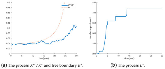
Figure 1. Simulation of the processes $X^m/K^{*}$ and $L^{*}$. The base parameters are as follows: x = 40, $k=200,T=30,\mu =0.1,\beta =0.08,\delta =0,\sigma =0.2,\gamma =0.5\mathrm{and}p=1.$

5. Concluding Remarks

In this paper, we studied an irreversible optimal investment problem with the finite horizon. To model the optimal invest problem, there have been many approaches—a stochastic control problem, dynamic programming techniques, the Bank–El Karoui representation theorem, etc. Among them, we consider the HJB equation as a singular stochastic control problem. In fact, in the mathematical economic literature, the singular stochastic control problems have been often used the irreversible optimal investment problem under an uncertain environment (See [16,18,21,23]). We dealt with a free boundary problem arising from the irreversible investment problem using the HJB equation.

We derived the integral equation for optimal irreversible investment with a finite horizon by the PDE approach. The dynamic capacity production of the firm was assumed to follow a geometric Brownian motion (GBM) process, and the Cobb–Douglas production function was used for the operating profit of the firm. To obtain the integral equation from the PDE for optimal investment, we used the Mellin transforms. The integral equation derived from the PDE was solved by using the recursive integration method. In other words, we solved numerically the integral equation for optimal irreversible investment. We also provided the graph to illustrate the movements of free boundaries for optimal investment with respect to time to maturity.

References

- Abel, A.B.; Eberly, J.C. Optimal investment with costly reversibility. Rev. Econ. Stud. 1996, 63, 581–593. [Google Scholar] [CrossRef]
- Eberly, J.C.; Mieghem, J.A.V. Multi-factor Dynamic Investment under Uncertainty. J. Econ. Theory 1997, 75, 345–387. [Google Scholar] [CrossRef]
- Bertola, G. Irreversible investment. Res. Econ. 1998, 52, 3–37. [Google Scholar] [CrossRef]
- Dangl, T. Investment and capacity choice under uncertain demand. Eur. J. Oper. Res. 1999, 117, 415–428. [Google Scholar] [CrossRef]
- Frontczak, R.; Schöbel, R. On modified Mellin transforms, Gauss-Laguerre quadrature, and the valuation of American call options. J. Comput. Appl. Math. 2010, 234, 1559–1571. [Google Scholar] [CrossRef][Green Version]
- Yoon, J.H. Mellin transform method for European option pricing with Hull-White stochastic interest rate. J. Appl. Math. 2017, 2017, 759562. [Google Scholar] [CrossRef]
- Jeon, J.; Han, H.; Kim, H.U.; Kang, M. An integral equation representation approach for Russian options with finite time horizon. Commun. Nonlinear Sci. 2016, 36, 496–516. [Google Scholar] [CrossRef]
- Jeon, J.; Yoon, J.H. Pricing external-chained barrier options with exponential barriers. Bull. Korean Math. Soc. 2016, 53, 1497–1530. [Google Scholar] [CrossRef]
- Jeon, J.; Han, H.; Kang, M. Valuing American floating strike lookback option and Neumann problem for inhomogeneous Black-scholes equation. J. Comput. Appl. Math. 2017, 313, 218–234. [Google Scholar] [CrossRef]
- Yoon, J.H.; Kim, J.-H. The pricing of vulnerable options with double Mellin transforms. J. Math. Anal. Appl. 2015, 422, 838–857. [Google Scholar] [CrossRef]
- Jeon, J.; Yoon, J.H.; Kang, M. Valuing vulnerable geometric Asian options. Comput. Math. Appl. 2016, 71, 676–691. [Google Scholar] [CrossRef]
- Kim, G.; Koo, E. Closed-form pricing formula for exchange option with credit risk. Chaos Soliton Fract. 2016, 91, 221–227. [Google Scholar] [CrossRef]
- Jeon, J.; Yoon, J.H.; Kang, M. Pricing vulnerable path-dependent options using integral transforms. J. Comput. Appl. Math. 2017, 313, 259–272. [Google Scholar] [CrossRef]
- Jeon, J.; Kim, G. Pricing of vulnerable options with early counterparty credit risk. N. Am. J. Econ. Financ. 2019, 47, 645–656. [Google Scholar] [CrossRef]
- Jeon, J.; Choi, S.Y.; Yoon, J.H. Analytic valuation of European continuous-installment barrier options. J. Comput. Appl. Math. 2020, 363, 392–412. [Google Scholar] [CrossRef]
- Chiarolla, M.B.; Haussmann, U.G. On a Stochastic, Irreversible Investment Problem. SIAM J. Control Optim. 2009, 48, 438–462. [Google Scholar] [CrossRef]
- Ewald, C.-O.; Wang, W.-K. Irreversible investment with Cox-Ingersoll-Ross type mean reversion. Math. Soc. Sci. 2010, 59, 314–318. [Google Scholar] [CrossRef]
- Riedel, F.; Su, X. On irreversible investment. Financ. Stoch. 2011, 15, 607–633. [Google Scholar] [CrossRef]
- Chiarolla, M.; Ferrari, G.; Riedel, F. Generalized Kuhn–Tucker conditions for n-firm stochastic irreversible investment under limited resources. SIAM J. Control Optim. 2013, 51, 3863–3885. [Google Scholar] [CrossRef]
- Chiarolla, M.; Ferrari, G. Identifying the free boundary of a stochastic, irreversible investment problem via the BankEl Karoui representation theorem. SIAM J. Control Optim. 2014, 52, 1048–1070. [Google Scholar] [CrossRef]
- Ferrari, G. On an integral equation for the free-boundary of stochastic, irreversible investment problems. Ann. Appl. Probab. 2015, 25, 150–176. [Google Scholar] [CrossRef]
- Ferrari, G.; Salminen, P. Irreversible investment under Lévy uncertainty: An equation for the optimal boundary. Adv. Appl. Probab. 2016, 48, 298–314. [Google Scholar] [CrossRef]
- Angelis, T.D.; Federico, S.; Ferrari, G. Optimal Boundary Surface for Irreversible Investment with Stochastic Costs. Math. Oper. Res. 2017, 42, 1135–1161. [Google Scholar] [CrossRef]
- Christensen, S.; Salminen, P. Multidimensional investment problem. Math. Financ. Econ. 2018, 12, 75–95. [Google Scholar] [CrossRef]
- Federico, S.; Rosestolato, M.; Tacconi, E. Irreversible investment with fixed adjustment costs: A stochastic impulse control approach. Math. Financ. Econ. 2019, 13, 579–616. [Google Scholar] [CrossRef]
- Jeon, J.; Kim, G. An integral equation approach for optimal investment policies with partial reversibility. Chaos Soliton Fract. 2019, 125, 73–78. [Google Scholar] [CrossRef]
- Fleming, W.H.; Soner, H.M. Controlled Markov Processes and Viscosity Solutions; Springer: New York, NY, USA, 2006. [Google Scholar]
- Guo, X.; Miao, J.; Morellec, E. Irreversible investment with regime shifts. J. Econ. Theory 2005, 122, 37–59. [Google Scholar] [CrossRef]
- Huang, J.; Subrahmanyam, M.; Yu, G. Pricing and hedging American options: A recursive integration method. Rev. Financ. Stud. 1996, 9, 277–300. [Google Scholar] [CrossRef]
- Lions, P.L.; Snitaman, A.S. Stochastic differential equations with reflecting boundary conditions. Commun. Pure Appl. Math. 1984, 37, 511–537. [Google Scholar] [CrossRef]
Publisher’s Note: MDPI stays neutral with regard to jurisdictional claims in published maps and institutional affiliations. |
© 2020 by the authors. Licensee MDPI, Basel, Switzerland. This article is an open access article distributed under the terms and conditions of the Creative Commons Attribution (CC BY) license (http://creativecommons.org/licenses/by/4.0/).