Multiple Outlier Detection Tests for Parametric Models

Abstract

We propose a simple multiple outlier identification method for parametric location-scale and shape-scale models when the number of possible outliers is not specified. The method is based on a result giving asymptotic properties of extreme z-scores. Robust estimators of model parameters are used defining z-scores. An extensive simulation study was done for comparing of the proposed method with existing methods. For the normal family, the method is compared with the well known Davies-Gather, Rosner’s, Hawking’s and Bolshev’s multiple outlier identification methods. The choice of an upper limit for the number of possible outliers in case of Rosner’s test application is discussed. For other families, the proposed method is compared with a method generalizing Gather-Davies method. In most situations, the new method has the highest outlier identification power in terms of masking and swamping values. We also created R package outliersTests for proposed test.

1. Introduction

The problem of multiple outliers identification received attention of many authors. The majority of outlier identification methods define rules for the rejection of the most extreme observations. The bulk of publications are concentrated on the normal distribution (see [1,2,3,4,5,6], see surveys in [7,8]. For non-normal case, the most of the literature pertains to the exponential and gamma distributions, see [9,10,11,12,13,14,15,16,17]. Outliers identification is important analyzing data collected in wide range of areas: pollution [18], IoT [19], medicine [20], fraud [21], smart city applications [22], and many more.

Constructing outlier identification methods, most authors suppose that the number s of observations suspected to be outliers is specified. These methods have a serious drawback: only two possible conclusions are done: exactly s observations are admitted as outliers or it is concluded that outliers are absent. More natural is to consider methods which do not specify the number of suspected observations or at least specify the upper limit s for it. Such methods are not very numerous and they concern normal or exponential samples. These are [1,5,23] methods for normal samples, [15,16,24] methods for exponential samples. The only method which does not specify the upper limit s is the [2] method for normal samples.

We give a competitive and simple method for outlier identification in samples from location-scale and shape-scale families of probability distributions. The upper limit s is not specified, as in the the case of Davies-Gather method. The method is based on a theorem giving asymptotic properties of extreme z-scores. Robust estimators of model parameters are used defining z-scores.

The following investigation showed that the proposed outlier identification method has superior performance as compared to existing methods. The proposed method widens considerably the scope of models applied in statistical analysis of real data. Differently from the normal probability distribution family many two-parameter families such as Weibull, logistic and loglogistic, extreme values, Cauchy, Laplace and other families can be applied for outlier identification. So it may be useful for models which cannot be symmetrized by simple transformations such as log-transform or others.

An advantage of the new method is that complicated computing is not needed because search of test statistic’s critical values by simulation is not needed for each sample size. It allowed to create an R package outliersTests which can be used for outlier search in real datasets. Another advantage is a very good potential for generalizations of the proposed method to regression, time series and other models. To have a competitor, we present not only the new method but also generalize the Davies-Gather method for non-normal data.

In Section 2 we present a short overview of the notion of the outlier region given by [2]. In Section 3 we give asymptotic properties of extreme z-scores based on equivariant estimators of model parameters, and introduce a new outlier identification method for parametric models based on the asymptotic result and robust estimators. In Section 4 we consider rather evident generalizations of Davies-Gather tests for normal data to location-scale families. In Section 5 we give a short overview of known multiple outlier identification methods for normal samples which do not specify an exact number of suspected outliers. In Section 6 we compare performance of the new and existing methods.

2. Outliers and Outlier Regions

Suppose that data are independent random variables $X_1,\dots ,X_n$. Denote by $F_i\left(x\right)$ the c.d.f. of $X_i$.

Let ${\mathcal{F}}_0=\{F(x,\theta ),\theta \in \mathrm{\Theta }\subset {\mathbf{R}}^m\}$ be a parametric family of absolutely continuous cumulative distribution functions with continuous unimodal densities f on the support $supp\left(F\right)$ of the c.d.f. F.

Suppose that if the data are not contaminated with unusual observations, then the following null hypothesis ${\mathrm{H}}_0$ is true: there exist $\theta \in \mathrm{\Theta }$ such that

$$F_1\left(x\right)=\dots =F_n\left(x\right)=F(x,\theta ).$$

(1)

There are two different definitions of an outlier. In the first case the outlier is an observation which falls into some outlier region $out\left(X\right)$. The outlier region is a set such that the probability for at least one observation from a sample to fall into it is small if the hypothesis ${\mathrm{H}}_0$ is true. In such a case the probability that a specified observation $X_i$ falls into $out\left(X\right)$ is very small. If an observation $X_i$ has distribution different from that under ${\mathrm{H}}_0$ then this probability may be considerably higher.

In the second case, the value $x_i$ of $X_i$ is an outlier if the probability distribution of $X_i$ is different from that under ${\mathrm{H}}_0$, formally $F_i\ne F(x,\theta )$. In this case, outliers are often called contaminants.

Therefore, in the first case, there exists a very small probability to have an outlier under ${\mathrm{H}}_0$. If the hypothesis ${\mathrm{H}}_0$ holds, then contaminants are absent and with very small probability some outliers (in the first sense) are possible. If contaminants are present, then the hypothesis ${\mathrm{H}}_0$ is not true. Nevertheless, contaminants are not necessary outliers (in the first sense ) because it is possible that they do not fall into the outlier region. So the two notions are different. Both definitions give approximately the same outliers if the alternative distribution is concentrated in the outlier region. Namely such contaminants can be called outliers in the sense that outliers are anomalous extreme observations. In such a case it is possible to compare outlier and contaminant search methods.

In this paper, we consider location-scale and shape-scale families. Location-scale families have the form ${\mathcal{F}}_{ls}=\{F_0((x-\mu )/\sigma ),\mu \in \mathbf{R},\sigma >0\}$ with the completely specified baseline c.d.f $F_0$ and p.d.f. $f_0$. Shape-scale families have the form ${\mathcal{F}}_{ls}=\{G_0(\left({(x/\theta )}^{\nu }\right),\theta ,\nu >0\}$ with completely specified baseline c.d.f $G_0$ and p.d.f. $g_0$. By logarithmic transformation the shape-scale families are transformed to location-scale family, so we concentrate on location-scale families. Methods for such families are easily modified to methods for shape-scale families.

The right-sided $\alpha$-outlier region for a location-scale family is

$$ou{t}_r({\alpha }_n,F)=\{x\in \mathbf{R}:x>\mu +\sigma F_0^{-1}(1-\alpha )\}$$

and the left-sided $\alpha$-outlier region is

$$ou{t}_l({\alpha }_n,F)=\{x\in \mathbf{R}:x<\mu +\sigma F_0^{-1}\left(\alpha \right)\}.$$

The two-sided $\alpha$-outlier region has the form

$$out(\alpha ,F)=\{x\in \mathbf{R}/[\mu +\sigma F_0^{-1}(\alpha /2),\mu +\sigma F_0^{-1}(1-\alpha /2)]\}.$$

(2)

If $f_0$ is symmetric, then the two-sided outlier region is simpler:

$$out(\alpha ,F)=\{x\in \mathbf{R}:|x-\mu |>\sigma F_0^{-1}(1-\alpha /2)\}.$$

The value of $\alpha$ is chosen depending on the size n of a sample: $\alpha ={\alpha }_n$. The choice is based on assumption that under ${\mathrm{H}}_0$ for some $\overline{\alpha }$ close to zero

$$\begin{array}{c}\hfill \mathbf{P}\left\{{\cap }_{i=1}^n\{X_i\notin out({\alpha }_n,F)\}\right\}={\left(\mathbf{P}\{X_i\notin out({\alpha }_n,F)\}\right)}^n=1-\overline{\alpha }.\end{array}$$

(3)

The equality (3) means that under ${\mathrm{H}}_0$ the probability that none of $X_i$ falls into ${\alpha }_n$-outlier region is $1-\overline{\alpha }$. It implies that

$${\alpha }_n=1-{(1-\overline{\alpha })}^{1/n}.$$

(4)

The sequence ${\alpha }_n$ decreases from $\overline{\alpha }$ to 0 as n goes from 1 to ∞.

The first definition of an outlier is as follows: for a sample size n a realization $x_i$ of $X_i$ is called outlier if $x_i\in out({\alpha }_n,F)$; $x_i$ is called right outlier if $x_i\in ou{t}_r({\alpha }_n,F)$.

The number of outliers $D_n$ under ${\mathrm{H}}_0$ has the binomial distribution $B(n,{\alpha }_n)$ and the expected number of outliers in the sample under ${\mathrm{H}}_0$ is $\mathbf{E}{D}_n=n{\alpha }_n.$ Please note that $\mathbf{E}{D}_n\to -ln(1-\overline{\alpha })\approx \overline{\alpha }$ as $n\to \infty$. For example, if $\overline{\alpha }=0.05$, then $ln(1-\overline{\alpha })\approx 0.05129$ and for $n\ge 10$ the expected number of outliers is approximately $0.051$, i.e., it practically does not depend on n. So under ${\mathrm{H}}_0$ the expected number of outliers $0.051$ is negligible with respect to the sample size n.

3. New Method

3.1. Preliminary Results

Suppose that a c.d.f. $F\in {\mathcal{F}}_{ls}$ belongs also to the domain of attraction ${\mathcal{G}}_{\gamma }$, $\gamma \ge 0$ (see [25]).

If $F\in {\mathcal{G}}_0\cap {\mathcal{F}}_{ls}$, then there exist normalizing constants $a_n>0$ and $b_n\in \mathbf{R}$ such that ${lim}_{n\to \infty }{F}_0^n(a_{n}x+b_n)=e^{-e^{-x}}.$ Similarly, if $F\in {\mathcal{G}}_{\gamma }\cap {\mathcal{F}}_{ls}$, $\gamma >0$, then ${lim}_{n\to \infty }{F}_0^n(a_{n}x+b_n)=e^{-{(-x)}^{-1/\gamma }},\hspace{1em}x<0$, ${lim}_{n\to \infty }{F}^n(a_{n}x+b_n)=1,x\ge 0.$

One of possible choices of the sequences $\left\{b_n\right\}$ and $\left\{a_n\right\}$ is

$$b_n=F_0^{-1}(1-\frac{1}{n}),\hspace{1em}{a}_n=1/\left(n{f}_0\left(b_n\right)\right).$$

(5)

In the particular case of the normal distribution equivalent form $a_n=1/b_n$ can be used. Expressions of $b_n$ and $a_n$ for some most used distributions are given in Table 1.

Table 1. Expressions of $b_n$ and $a_n$.

Distribution	${\mathit{F}}_0\left(\mathit{x}\right)$	${\mathit{b}}_{\mathit{n}}$	${\mathit{a}}_{\mathit{n}}$
Normal	$\mathsf{\Phi }\left(x\right)$	${\mathsf{\Phi }}^{-1}(1-1/n)$	$1/b_n$
Type I extreme value	$1-e^{-e^x}$	$lnlnn$	$e^{-b_n}$
Type II extreme value	$e^{-e^{-x}}$	$ln(-ln(1-1/n\left)\right)$	$e^{b_n}/(n-1)$
Logistic	$\frac{1}{1+e^{-x}}$	$ln(n-1)$	$n/\left(n-1\right)$
Laplace	$\frac{1}{2}+\frac{1}{2}\mathrm{sign}\left(x\right)(1-e^{-|x|})$	$ln(n/2)$	1
Cauchy	$\frac{1}{2}+\frac{1}{\pi }arctan\left(x\right)$	$cot\left(\frac{\pi }{n}\right)$	$\frac{\pi }{n}/{sin}^2\left(\frac{\pi }{n}\right)$

Condition A.

(a) 

$\widehat{\mu }$ and $\widehat{\sigma }$ are consistent estimators of μ and σ;

(b) 

the limit distribution of ($\sqrt{n}(\widehat{\mu }-\mu ),\sqrt{n}(\widehat{\sigma }-\sigma ))$ is non-degenerate;

(c) 

$$\underset{x\to \infty }{lim}\frac{x{f}_0\left(x\right)}{\sqrt{1-F_0\left(x\right)}}=0.$$

Condition A (c) is satisfied for many location-scale models including the normal, type I extreme value, type II extreme value, logistic, Laplace ($F\in {\mathcal{G}}_0$), Cauchy ($F\in {\mathcal{G}}_1$).

Set $Y_i=(X_i-\mu )/\sigma$, ${\widehat{Y}}_i=(X_i-\widehat{\mu })/\widehat{\sigma }$. The random variables ${\widehat{Y}}_i$ are called z-scores. Denote by $Y_{\left(1\right)}\le Y_{\left(2\right)}\le \dots \le Y_{\left(n\right)}$ and ${\widehat{Y}}_{\left(1\right)}\le \dots \le {\widehat{Y}}_{\left(n\right)}$ the respective order statistics

The following theorem is useful for right outliers detection test construction.

Theorem 1.

If $F\in {\mathcal{G}}_0\cap {\mathcal{F}}_{ls}$ and Conditions A hold, then for fixed s

$$(({\widehat{Y}}_{\left(n\right)}-b_n)/a_n,({\widehat{Y}}_{(n-1)}-b_n)/a_n,\dots ,({\widehat{Y}}_{(n-s+1)}-b_n)/a_n)\stackrel{d}{\to }$$

$$L_0=(-ln{E}_1,-ln(E_1+E_2),\dots ,-ln(E_1+\dots +E_s))$$

as $n\to \infty$, where $E_1,\dots ,E_s$ are i.i.d. standard exponential random variables.

If $F\in {\mathcal{G}}_{\gamma }\cap {\mathcal{F}}_{ls}$, $\gamma >0$ and Conditions A hold, then the limit random vector is

$$L_{\gamma }=(E_1^{-1}-1,{(E_1+E_2)}^{-1}-1,\dots ,{(E_1+\dots +E_s)}^{-1}-1).$$

Proof of Theorem 1.

Please note that

$$\frac{{\widehat{Y}}_{(n-i+1)}-b_n}{a_n}=\frac{Y_{(n-i+1)}-b_n}{a_n} \frac{\sigma }{\widehat{\sigma }}+\frac{(\mu -\widehat{\mu })}{\widehat{\sigma }{a}_n}+\frac{b_n}{a_n}\frac{\sigma -\widehat{\sigma }}{\widehat{\sigma }}$$

The s-dimensional random vector such that its ith component is the first term of the right side converges in distribution to the random vector given in the formulation of the theorem. It follows from Theorem 2.1.1 of [25] and Condition A (a). So it is sufficient to show that the second and the third terms converge to zero in probability. The second term is

$$-\sqrt{n}{f}_0\left(F_0^{-1}(1-\frac{1}{n})\right)\frac{\sqrt{n}(\widehat{\mu }-\mu )}{\widehat{\sigma }},$$

the third term is

$$-\sqrt{n}{F}_0^{-1}(1-\frac{1}{n})f_0\left(F_0^{-1}(1-\frac{1}{n})\right)\frac{\sqrt{n}(\widehat{\sigma }-\sigma )}{\widehat{\sigma }}.$$

By Condition A (c)

$$\underset{n\to \infty }{lim}\sqrt{n}{F}_0^{-1}(1-\frac{1}{n})f_0\left(F_0^{-1}(1-\frac{1}{n})\right))=\underset{x\to \infty }{lim}\frac{x{f}_0\left(x\right)}{\sqrt{1-F_0\left(x\right)}}=0.$$

It also implies ${lim}_{n\to \infty }\sqrt{n}{f}_0\left(F_0^{-1}(1-\frac{1}{n})\right)=0$ because ${lim}_{n\to \infty }{F}_0^{-1}(1-\frac{1}{n})=\infty .$ Proof completed. □

Remark 1.

Please note that $2(E_1+\dots +E_i)\sim {\chi }^2\left(2i\right)$. It implies that if $F\in {\mathcal{G}}_0\cap {\mathcal{F}}_{ls}$, then for fixed i, $i=1,\dots ,s$,

$$\mathbf{P}\{({\widehat{Y}}_{(n-i+1)}-b_n)/a_n\le x\}\to 1-F_{{\chi }_{2i}^2}\left(2e^{-x}\right)\hspace{1em}as\hspace{1em}n\to \infty .$$

(6)

Similarly, if $F\in {\mathcal{G}}_{\gamma }\cap {\mathcal{F}}_{ls}$, $\gamma >0$, then for fixed i, $i=1,\dots ,s$,

$$\mathbf{P}\{({\widehat{Y}}_{(n-i+1)}-b_n)/a_n\le x\}\to 1-F_{{\chi }_{2i}^2}\left(\frac{2}{1+x}\right)\hspace{1em}as\hspace{1em}n\to \infty .$$

(7)

The following theorem is useful for construction of outlier detection tests in two-sided case when $f_0$ is symmetric. For any sequence ${\zeta }_1,\dots ,{\zeta }_n$ denote by ${|\zeta |}_{\left(1\right)}\le \dots \le {|\zeta |}_{\left(n\right)}$ the ordered absolute values $|{\zeta }_1|,\dots ,|{\zeta }_n|$.

Theorem 2.

Suppose that the function $f_0$ is symmetric. If $F\in {\mathcal{G}}_{\gamma }\cap {\mathcal{F}}_{ls}$, $\gamma \ge 0$ and Conditions A hold, then for fixed s

$$\left(\right(|\widehat{Y}{|}_{\left(n\right)}-b_{2n})/a_{2n},(|\widehat{Y}{|}_{(n-1)}-b_{2n})/a_{2n},\dots ,(|\widehat{Y}{|}_{(n-s+1)}-b_{2n})/a_{2n})\stackrel{d}{\to }{L}_{\gamma }$$

as $n\to \infty$.

Proof of Theorem 2.

For any $i=1,\dots ,s$ the following equality holds:

$$\frac{|\widehat{Y}{|}_{(n-i+1)}-b_{2n}}{a_{2n}}=\frac{|\widehat{Y}{|}_{(n-i+1)}-{|Y|}_{(n-i+1)}}{a_{2n}}+\frac{{|Y|}_{(n-i+1)}-b_{2n}}{a_{2n}}.$$

(8)

The c.d.f. of the random variables $|Y_i|$ is $2F_0\left(x\right)-1$, so if $F_0\in {\mathcal{G}}_{\gamma }$, $\gamma \ge 0$ then $2F_0-1\in {\mathcal{G}}_{\gamma }$, and for the sequence $|Y_n|$ the normalizing sequences are $a_{2n},b_{2n}$. So the s-dimensional random vector such that its ith component is the second term of the right side converges in distribution to the random vector given in the formulation of the theorem. It follows from Theorem 2.1.1 of [25]. So it is sufficient to show that the first term converges in probability to zero.

Please note that $|{\widehat{Y}}_i|\le |Y_i|+|{\widehat{Y}}_i-Y_i|$, and

$$|{\widehat{Y}}_i-Y_i|=\frac{1}{\widehat{\sigma }}|\mu -\widehat{\mu }+(\sigma -\widehat{\sigma })Y_i|\le \frac{|\widehat{\mu }-\mu |}{\widehat{\sigma }}+\frac{|\sqrt{n}(\widehat{\sigma }-\sigma )|}{\widehat{\sigma }}\frac{1}{\sqrt{n}}{|Y|}_{\left(n\right)}.$$

So $|\widehat{Y}{|}_{(n-j+1)}\le {|Y|}_{(n-j+1)}+\frac{|\widehat{\mu }-\mu |}{\widehat{\sigma }}+\frac{|\sqrt{n}(\widehat{\sigma }-\sigma )|}{\widehat{\sigma }}\frac{1}{\sqrt{n}}{|Y|}_{\left(n\right)}.$ Analogously, the inequality $Y_i|\le ||{\widehat{Y}}_i|+|{\widehat{Y}}_i-Y_i|$ implies that ${|Y|}_{(n-j+1)}\le |\widehat{Y}{|}_{(n-j+1)}+\frac{|\widehat{\mu }-\mu |}{\widehat{\sigma }}+\frac{|\sqrt{n}(\widehat{\sigma }-\sigma )|}{\widehat{\sigma }}\frac{1}{\sqrt{n}}{|Y|}_{\left(n\right)}.$

Theorem 2.1.1 in [25] applied to the random variables $|Y_i|$ implies that there exist a random variable $V_1$ with the c.d.f. $G\left(x\right)=e^{-e^{-x}}$ ($\gamma =0$) or $G\left(x\right)=e^{-{(-x)}^{-1/\gamma }},x<0$, $G\left(x\right)=1$, $x\ge 0$ ($\gamma >0$), such that

$$\frac{1}{\sqrt{n}}{|Y|}_{\left(n\right)}=(b_{2n}+a_{2n}(V_1+o_P\left(1\right)))/\sqrt{n}.$$

(9)

$$|\frac{|\widehat{Y}{|}_{(n-i+1)}-{|Y|}_{(n-i+1)}}{a_{2n}}|\le \frac{|\sqrt{n}(\widehat{\mu }-\mu )|}{\widehat{\sigma }\sqrt{n}{a}_{2n}}+\frac{|\sqrt{n}(\widehat{\sigma }-\sigma )|}{\widehat{\sigma }}(\frac{b_{2n}}{\sqrt{n}{a}_{2n}}+\frac{V_1+o_p\left(1\right)}{\sqrt{n}}).$$

The convergence $b_n\to \infty$ and Condition A (c) imply:

$$\underset{n\to \infty }{lim}\frac{b_{2n}}{\sqrt{n}{a}_{2n}}=\underset{n\to \infty }{lim}\sqrt{n}{F}_0^{-1}(1-\frac{1}{2n})f_0{F}_0^{-1}(1-\frac{1}{2n}))=$$

$$\frac{1}{\sqrt{2}}\underset{x\to \infty }{lim}\frac{x{f}_0\left(x\right)}{\sqrt{1-F_0\left(x\right)}}=0,\hspace{1em}\underset{n\to \infty }{lim}\frac{1}{\sqrt{n}{a}_{2n}}=0.$$

These results and Conditions A (a), (b) imply that the first term at the right of (8) converges in probability to zero. Proof completed. □

Remark 2.

Theorem 2 implies that if $F\in {\mathcal{G}}_0\cap {\mathcal{F}}_{ls}$, $n\to \infty$, then for fixed i, $i=1,\dots ,s$,

$$\mathbf{P}\left\{\right(|\widehat{Y}{|}_{(n-i+1)}-b_{2n})/a_{2n}\le x\}\to 1-F_{{\chi }_{2i}^2}\left(2e^{-x}\right),$$

(10)

and if $F\in {\mathcal{G}}_{\gamma }\cap {\mathcal{F}}_{ls}$, $\gamma >0$, then

$$\mathbf{P}\left\{\right(|\widehat{Y}{|}_{(n-i+1)}-b_{2n})/a_{2n}\le x\}\to 1-F_{{\chi }_{2i}^2}(2/(1+x)).$$

(11)

Suppose now that the function $f_0$ is not symmetric. Set $Y_i^{*}=-(X_i-\mu )/\sigma$. The c.d.f. and p.d.f. of $Y_i^{*}$ are $1-F_0(-x)$ and $f_0(-x)$, respectively. Set

$$b_n^{*}=-F_0^{-1}(1/n),\hspace{1em}{a}_n^{*}=1/\left(n{f}_0(-b_n^{*})\right).$$

(12)

For example, if type I extreme value distribution is considered, then

$$b_n=lnlnn,\hspace{1em}{a}_n=\frac{1}{lnn},\hspace{1em}{b}_n^{*}=-ln(-ln(1-\frac{1}{n})),\hspace{1em}{a}_n^{*}=-\frac{1}{(n-1)ln(1-\frac{1}{n})}.$$

For the type II extreme value distribution $a_n,b_n,a_n^{*},b_n^{*}$ have the same expressions as $a_n^{*},b_n^{*},a_n,b_n$ for the Type I extreme value distribution, respectively.

Remark 3.

Similarly as in Theorem 1 we have that if s is fixed and $F\in {\mathcal{G}}_0\cap {\mathcal{F}}_{ls}$, then for fixed i, $i=1,\dots ,s$,

$$\mathbf{P}\{(Y_{\left(i\right)}+b_n^{*})/(-a_n^{*})\le x\}=\mathbf{P}\{({\widehat{Y}}_{(n-i+1)}^{*}-b_n^{*})/a_n^{*}\le x\}\to 1-F_{{\chi }_{2i}^2}\left(2e^{-x}\right),$$

(13)

and if $F\in {\mathcal{G}}_{\gamma }\cap {\mathcal{F}}_{ls}$, $\gamma >0$, then for fixed i, $i=1,\dots ,s$,

$$\mathbf{P}\{(Y_{\left(i\right)}+b_n^{*})/(-a_n^{*})\le x\}=\mathbf{P}\{({\widehat{Y}}_{(n-i+1)}^{*}-b_n^{*})/a_n^{*}\le x\}\to 1-F_{{\chi }_{2i}^2}(2/(1+x)).$$

(14)

3.2. Robust Estimators for Location-Shape Distributions

The choice of the estimators $\widehat{\mu }$ and $\widehat{\sigma }$ is important when outlier detection problem is considered. The ML estimators from the complete sample are not stable when outliers exist.

In the case of location-scale families highly efficient robust estimators of the location and scale parameters $\mu$ and $\sigma$ are (see [26])

$$\widehat{\mu }=MED-\widehat{\sigma }{F}_0^{-1}\left(0.5\right),\hspace{1em}\widehat{\sigma }=Q_n=d W_{\left(\right[0.25n(n-1)/2\left]\right)},$$

(15)

where $MED$ is the empirical median, $W_{ij}=|X_i-X_j|,\hspace{1em}1\le i<j\le n$ are $C_n^2=n(n-1)/2$ absolute values of the differences $X_i-X_j$ and $W_{\left(l\right)}$ is the lth order statistic from $W_{ij}$.

The constant d has the form $d=1/K_0^{-1}(5/8)$, where $K_0^{-1}\left(x\right)$ is the inverse of the c.d.f. of $Y_1-Y_2$, $Y_i=(X_i-\mu )/\sigma \sim F_0\left(x\right)$.

Expressions of $K_0^{-1}\left(x\right)$ and values d for some well-known location-scale families are given in Table 2.

Table 2. Values of d for various probability distributions.

Distribution	${\mathit{K}}_0\left(\mathit{x}\right)$	d
Normal	$\mathsf{\Phi }(x/\sqrt{2})$	2.2219
Type I extr.val.	$1/(1+e^{-x})$	1.9576
Type II extr.val.	$1/(1+e^{-x})$	1.9576
Logistic	$1-\frac{(x-1)e^x+1}{{(e^x-1)}^2}$	1.3079
Laplace	$1-\frac{1}{2}(1+\frac{x}{2})e^{-x}$	1.9306
Cauchy	$\frac{1}{2}+\frac{1}{\pi }arctan(x/2)$	1.2071

The above considered estimators are equivariant under ${\mathrm{H}}_0$, i.e. for any $e\in \mathbf{R},f>0$, the following equalities hold:

$$\widehat{\mu }((X_1-e)/f,\dots ,(X_n-e)/f)=(\widehat{\mu }(X_1,\dots ,X_n)-e)/f,$$

$$\widehat{\sigma }((X_1-e)/f,\dots ,(X_n-e)/f)=\widehat{\sigma }(X_1,\dots ,X_n)/f.$$

Equivariant estimators have the following property: the distribution of $(\widehat{\mu }-\mu )/\sigma$, $\widehat{\sigma }/\sigma$ and $(\widehat{\mu }-\mu )/\widehat{\sigma }$ does not depend on the values of the parameters $\mu$ and $\sigma$.

3.3. Right Outliers Identification Method for Location-Scale Families

Suppose that $F\in {\mathcal{G}}_{\gamma }\cap {\mathcal{F}}_{ls}$, $\gamma \ge 0$. Let $a_n,b_n$ be defined by (5). Set

$$U_{(n-i+1)}^{+}\left(n\right)=1-F_{{\chi }_{2i}^2}\left(2e^{-({\widehat{Y}}_{(n-i+1)}-b_n)/a_n}\right),\hspace{0.17em}\gamma =0,$$

$$U_{(n-i+1)}^{+}\left(n\right)=1-F_{{\chi }_{2i}^2}(2/(1+({\widehat{Y}}_{(n-i+1)}-b_n)/a_n),\hspace{0.17em}\gamma >0,$$

$$U^{+}(n,s)=\underset{1\le i\le s}{max}{U}_{(n-i+1)}^{+}\left(n\right).$$

(16)

Theorem 3.

The distribution of the statistic $U^{+}(n,s)$ is parameter-free for any fixed n.

Proof of Theorem 3.

The result follows from the equality

$$\frac{{\widehat{Y}}_{(n-i+1)}-b_n}{a_n}=\frac{Y_{(n-i+1)}-b_n}{a_n}\frac{\sigma }{\widehat{\sigma }}+\frac{b_n}{a_n}(\frac{\sigma }{\widehat{\sigma }}-1)+\frac{1}{a_n}\frac{\mu -\widehat{\mu }}{\widehat{\sigma }},$$

equivariance of the estimators $\widehat{\mu }$, $\widehat{\sigma }$ and the fact that the distribution of the random vector ${(Y_1,\dots ,Y_n)}^T$ does not depend on the values of the parameters $\mu$ and $\sigma$. □

Denote by $u_{\alpha }^{+}(n,s)$ the $\alpha$ critical value of the statistic $U^{+}(n,s)$. Please note that it is exact, not asymptotic $\alpha$ critical value: $\mathbf{P}\{U^{+}(n,s)\ge u_{\alpha }^{+}(n,s)\}=\alpha$ under ${\mathrm{H}}_0$.

Theorem 1 implies that the limit distribution (as $n\to \infty$) of the random variable $U^{+}(n,s)$ coincides with the distribution of the random variable $V^{+}\left(s\right)={max}_{1\le i\le s}{V}_i^{+},$ where $V_i^{+}=1-F_{{\chi }_{2i}^2}\left(2(E_1+\dots +E_i)\right)$, $E_1,\dots ,E_s$ are i.i.d. standard exponential random variables. The random variables $V_1^{+},\dots ,V_s^{+}$ are dependent identically distributed and the distribution of each $V_i^{+}$ is uniform: $V_i^{+}\sim U(0,1)$.

Denote by $v_{\alpha }^{+}\left(s\right)$ the $\alpha$ critical values of the random variable $V^{+}\left(s\right)$. They are easily found by simulation many times generating s i.i.d. standard exponential random variables and computing values of the random variables $V^{+}\left(s\right)$.

Our simulations showed that the below proposed outlier identification methods based on exact and approximate critical values of the statistic $U^{+}(n,s)$ give practically the same results, so for samples of size $n\ge 20$ we recommend to approximate the $\alpha$-critical level of the statistic $U^{+}(n,s)$ by the critical values $v_{\alpha }^{+}\left(s\right)$ which depend only on s. We shall see that for the purpose of outlier identification only the critical values $v_{\alpha }^{+}\left(5\right)$ are needed. We found that the critical values $v_{\alpha }^{+}\left(5\right)$ are: $v_{0.1}^{+}\left(5\right)=0.9677$, $v_{0.05}^{+}\left(5\right)=0.9853$, $v_{0.01}^{+}\left(5\right)=0.9975$.

Our simulations showed that the performance of the below proposed outlier identification method based on exact and approximate critical values of the statistic $U^{+}(n,5)$ is similar for samples of size $n\ge 20$.

We write shortly $BP$-method for the below considered method.

$BP$ method for right outliers. Begin outlier search using observations corresponding to the largest values of ${\widehat{Y}}_i$. We recommend begin with five largest. So take $s=5$ and compute the values of the statistics

$$U^{+}(n,5)=\underset{1\le i\le 5}{max}{U}_{(n-i+1)}^{+}\left(n\right).$$

If $U^{+}(n,5)\le v_{\alpha }^{+}\left(5\right)$, then it is concluded that outliers are absent and no further investigation is done. Under ${\mathrm{H}}_0$ the probability of such event is approximately $1-\alpha$.

If $U^{+}(n,5)>v_{\alpha }^{+}\left(5\right)$, then it is concluded that outliers exist.

Please note that (see the classification scheme below) that if $U^{+}(n,5)>v_{\alpha }^{+}\left(5\right)$, then minimum one observation is declared as an outlier. So the probability to declare absence of outliers does not depend on the following classification scheme.

If it is concluded that outliers exist then search of outliers is done using the following steps.

Step 1. Set $d_1=max\{i\in \{1,\dots ,5\}:U_{(n-i+1)}^{+}\left(n\right)>v_{\alpha }^{+}\left(5\right)\}$. Please note that the maximum $d_1>0$ exists because $U^{+}(n,5)>v_{\alpha }^{+}\left(5\right)$.

If $d_1<5$, then classification is finished at this step: $d_1$ observations are declared as right outliers because if the value of $X_{(n-d_1)}$ is declared as an outlier, then it is natural to declare values of $X_{\left(n\right)},\dots ,X_{(n-d_1+1)}$ as outliers, too.

If $d_1=5$, then it is possible that the number of outliers is higher than 5. Then the observation corresponding to $i=1$ (i.e., corresponding to $X_{\left(n\right)}$) is declared as an outlier and we proceed to the step 2.

Step 2. The above written procedure is repeated taking $U^{+}(n-1,5)={max}_{1\le i\le 5}{U}_{(n-i)}^{+}(n-1)$ instead of $U^{+}(n,5)$; here

$$U_{(n-i)}^{+}(n-1)=1-F_{{\chi }_{2i}^2}\left(2e^{-({\widehat{Y}}_{(n-i)}-b_{n-1})/a_{n-1}}\right),\hspace{1em}i=1,\dots ,5,$$

Set $d_2=max\{i\in \{1,\dots ,5\}:U_{(n-i)}^{+}(n-1)>v_{\alpha }^{+}\left(5\right)\}$. If $d_2<5$, the classification is finished and $d_2+1$ observations are declared as outliers.

If $d_2=5$, then it is possible that the number of outliers is higher than 6. Then the observation corresponding to the largest ${\widehat{Y}}_{(n-1)}$ is declared as an outlier, in total 2 observations (i.e., the observations corresponding to $i=1,2$ (i.e., corresponding to $X_{\left(n\right)}$ and $X_{(n-1)}$) are declared as outliers and we proceed to the Step 3, and so on. Classification finishes at the lth step when $d_l<5$. So we declare $(l-1)$ outliers in the previous steps and $d_l$ outliers in the last one. The total number of observations declared as outliers is $l-1+d_l$. These observations are values of $X_{\left(n\right)},\dots ,X_{(n-d_l-l+2)}$.

3.4. Left Outliers Identification Method for Location-Scale Families

Let $a_n^{*},b_n^{*}$ be the normalizing constants defined by (12). If $F\in {\mathcal{G}}_0\cap {\mathcal{F}}_{ls}$, $i=1,\dots ,s$, then set

$$U_{\left(i\right)}^{-}\left(n\right)=1-F_{{\chi }_{2i}^2}\left(2e^{({\widehat{Y}}_{\left(i\right)}+b_n^{*})/a_n^{*}}\right),\hspace{1em}{U}^{-}(n,s)=\underset{1\le i\le s}{max}{U}_{\left(i\right)}^{-}\left(n\right).$$

If $F\in {\mathcal{G}}_{\gamma }\cap {\mathcal{F}}_{ls}$, $\gamma >0$, then replace $e^{({\widehat{Y}}_{\left(i\right)}+b_n^{*})/a_n^{*}}$ by $1/(1+({\widehat{Y}}_{\left(i\right)}+b_n^{*})/a_n^{*})$. Denote by $u_{\alpha }^{-}(n,s)$ the $\alpha$ critical value of the statistic $U^{-}(n,s)$.

Theorem 1 and Remark 3 imply that the limit distribution (as $n\to \infty$) of the random variable $U^{-}(n,s)$ coincides with the distribution of the random variable $V^{+}\left(s\right)$. So the critical values $u_{\alpha }^{-}(n,s)$ are approximated by the critical values $v_{\alpha }^{-}\left(s\right)=v_{\alpha }^{+}\left(s\right)$.

The left outliers search method coincides with the right outliers search method replacing + to − in all formulas.

3.5. Outlier Detection Tests for Location-Scale Families: Two-Sided Alternative, Symmetric Distributions

Let $a_n,b_n$ be defined by (5). If $F\in {\mathcal{G}}_0\cap {\mathcal{F}}_{ls}$, $i=1,\dots ,s$, then set

$$U_{(n-i+1)}\left(n\right)=1-F_{{\chi }_{2i}^2}\left(2e^{-(|\widehat{Y}{|}_{(n-i+1)}-b_{2n})/a_{2n}}\right),\hspace{1em}U(n,s)=\underset{1\le i\le s}{max}{U}_{(n-i+1)}\left(n\right).$$

If $F\in {\mathcal{G}}_{\gamma }\cap {\mathcal{F}}_{ls}$, $\gamma >0$, then replace $e^{({\widehat{Y}}_{\left(i\right)}+b_n^{*})/a_n^{*}}$ by $1/(1+({\widehat{Y}}_{\left(i\right)}+b_n^{*})/a_n^{*})$. Denote by $u_{\alpha }(n,s)$ the $\alpha$ critical value of the statistic $U(n,s)$.

Theorem 1 and Remark 2 imply that the limit distribution (as $n\to \infty$) of the random variable $U(n,s)$ coincides with the distribution of the random variable $V^{+}\left(s\right)$. So the critical values $u_{\alpha }(n,s)$ are approximated by the critical values $v_{\alpha }\left(s\right)=v_{\alpha }^{+}\left(s\right)$.

The outliers search method coincides with the right outliers search method skipping upper index + in all formulas.

3.6. Outlier Detection Tests for Location-Scale Families: Two-Sided Alternative, Non-Symmetric Distributions

Suppose now that the function $f_0$ is not symmetric. Let $a_n,b_n,a_n^{*},b_n^{*}$ be defined by (12).

Begin outlier search using observations corresponding to the largest and the smallest values of ${\widehat{Y}}_i$. We recommend begin with five smallest and five largest. So compute the values of the statistics $U^{-}(n,5)$ and $U^{+}(n,5)$. If $U^{-}(n,5)\le v_{\alpha /2}\left(5\right)$ and $U^{+}(n,5)\le v_{\alpha /2}\left(5\right)$, then it is concluded that outliers are absent and no further investigation is done.

If $U^{-}(n,5)>v_{\alpha /2}\left(5\right)$ or $U^{-}(n,5)>v_{\alpha /2}\left(5\right)$, then it is concluded that outliers exist. If $U^{-}(n,5)>v_{\alpha /2}\left(5\right)$, then left outliers are searched as in Section 3.3. If $U^{+}(n,5)>v_{\alpha /2}\left(5\right)$, then right outliers are searched as in Section 3.2. The only difference is that $\alpha$ is replaced by $\alpha /2$ in all formulas.

3.7. Outlier Identification Method for Shape-Scale Families

If shape-scale families of the form $\{F(t;\theta ,\nu )=G_0\left({(t/\theta )}^{\nu }\right),\hspace{0.17em}\theta ,\nu >0\}$ with specified $G_0$ are considered then the above given tests for location-scale families could be used because if $X_1,\dots ,X_n$ is a sample from shape scale family then $Z_1,\dots ,Z_n$, $Z_i=ln{X}_i$, is a sample from location-scale family $\left\{F_0((x-\mu )/\sigma ,\mu \in \mathbf{R},\sigma >0\}\right)$ with $\mu =ln\theta$, $\sigma =1/\nu$, $F_0\left(x\right)=G_0\left(e^x\right)$.

3.8. Illustrative Example

To illustrate simplicity of the $BP$-method, let us consider an illustrative example of its application (sample size $n=20$, $r=7$ outliers). The sample of size $n=20$ from standard normal distribution was generated. The 1st-3rd and 17th-20th observations were replaced by outliers. The observations $x_i$, the absolute values $|{\widehat{Y}}_i|$ of the z-scores ${\widehat{Y}}_i$, and the ranks $\left(i\right)$ of $|{\widehat{Y}}_i|$ are presented in Table 3.

Table 3. Illustrative sample ($n=20,r=7$).

i	${\mathit{x}}_{\mathit{i}}$	$|{\widehat{\mathit{Y}}}_{\mathit{i}}|$	$\left(\mathit{i}\right)$	i	${\mathit{x}}_{\mathit{i}}$	$|{\widehat{\mathit{Y}}}_{\mathit{i}}|$	$\left(\mathit{i}\right)$
1	6.10	3.18	16	11	−0.69	0.28	9
2	10	5.17	18	12	−0	0.07	5
3	6.20	3.23	17	13	0.05	0.10	6
4	−0.08	0.03	2	14	−0.20	0.03	1
5	0.63	0.39	11	15	−0.25	0.06	4
6	−0.54	0.21	7	16	−0.64	0.25	8
7	1.37	0.77	13	17	−6.30	3.14	15
8	0.46	0.30	10	18	−5.50	2.73	14
9	−0.22	0.04	3	19	−12.10	6.10	19
10	0.94	0.55	12	20	−20	10.13	20

In Table 4 we present steps of the classification procedure by the $BP$ method. First, we compute (see line 1 of Table 4) value of the statistic $U(20,5)={max}_{1\le i\le 5}{U}_{(20-i+1)}\left(20\right)=1$. Since $U(20,5)=1>0.9853=v_{0.05}\left(5\right)$, we reject the null hypothesis, conclude that outliers exist and begin the search of outliers.

Table 4. Illustrative example of $BP$ test observations classification.

$U_{\left(20\right)}\left(20\right)$	$U_{\left(19\right)}\left(20\right)$	$U_{\left(18\right)}\left(20\right)$	$U_{\left(17\right)}\left(20\right)$	$U_{\left(16\right)}\left(20\right)$	$U(20,5)$
1.000000	1.000000	1.000000	0.999998	1.000000	1.000000
$U_{\left(19\right)}\left(19\right)$	$U_{\left(18\right)}\left(19\right)$	$U_{\left(17\right)}\left(19\right)$	$U_{\left(16\right)}\left(19\right)$	$U_{\left(15\right)}\left(19\right)$	$U(19,5)$
0.999685	0.999998	0.999916	0.999998	1.000000	1.000000
$U_{\left(18\right)}\left(18\right)$	$U_{\left(17\right)}\left(18\right)$	$U_{\left(16\right)}\left(18\right)$	$U_{\left(15\right)}\left(18\right)$	$U_{\left(14\right)}\left(18\right)$	$U(18,5)$
0.998046	0.996970	0.999893	0.999997	0.999997	0.999997
$U_{\left(17\right)}\left(17\right)$	$U_{\left(16\right)}\left(17\right)$	$U_{\left(15\right)}\left(17\right)$	$U_{\left(14\right)}\left(17\right)$	$U_{\left(13\right)}\left(17\right)$	$U(17,5)$
0.924219	0.996446	0.999871	0.999940	0.084290	0.999940

Step 1. The inequality $U_{\left(16\right)}\left(20\right)=1.0000>0.9853=v_{0.05}\left(5\right)$ (note that $U_{\left(16\right)}\left(20\right)$ corresponds to the fifth largest observation in absolute value) implies that $d_1=5$. So it is possible that the number of outliers might be greater than 5. We reject the largest in absolute value 20th observation as an outlier and continue the search of outliers.

Step 2. The inequality $U_{\left(15\right)}\left(19\right)=1.0000>0.9853=v_{0.05}\left(5\right)$ (note that $U_{\left(15\right)}\left(19\right)$ corresponds to the fifth largest observation in absolute value from the remaining 19 observations) implies that $d_2=5$. So it is possible that the number of outliers might be greater than 6. We declare the second largest in absolute value observation as an outlier. So two observations (19th and 20th) are declared as outliers. We continue the search of outliers.

Step 3. The inequality $U_{\left(14\right)}\left(18\right)=0.999997>0.9853=v_{0.05}\left(5\right)$ implies that $d_3=5$. We declare the third largest in absolute value observation as an outlier. So three observations (2nd, 19th and 20th) are declared as outliers. We continue the search of outliers.

Step 4. The inequalities $U_{\left(13\right)}\left(17\right)=0.084290<0.9853=v_{0.05}\left(5\right)$ and $U_{\left(14\right)}\left(17\right)=0.999940>0.9853=v_{0.05}\left(5\right)$ imply that $d_4=4$. So four additional observations (the fourth, fifth, sixth and seventh largest in absolute value observations), namely the 3d, 1st, 17th, and 7th are declared as outliers, The outlier search is finished. In all, 7 observations were declared as outliers: 1–3,17–20, as was expected. Please note that since the outlier search procedure was done after rejection of the null hypothesis, the significance level did not change.

3.9. Practical Example

Let’s consider the stent fatigue testing dataset from reliability control [27]. The dataset contains 100 observations. Let us consider the Weibull, lollogistic and lognormal models. These are the most applied models for analysis of reliability data. For preliminary choice of suitable model we compare the values of various goodness-of-fit statistics and information criteria (see Table 5). The Weibull model is obviously the most suited because values of all five statistics are smallest for this model.

Table 5. Values of goodness-of-fit statistics and information criteria (initial sample).

Goodness-of-Fit Statistics	Weibull	Logistic	Log-Normal
Kolmogorov-Smirnov statistic	0.05	0.09	0.07
Cramer-von Mises statistic	0.03	0.23	0.127
Anderson-Darling statistic	0.21	1.36	1.08
Goodness-of-fit criteria
Akaike’s Information Criterion	1056.515	1074.783	1073.13
Bayesian Information Criterion	1061.725	1079.993	1078.34

Using the function WEDF.test from the R package EWGoF we applied the following goodness-of-fit tests for Weibull distribution: Anderson-Darling (p-value = 0.86), Kolmogorov-Smirnov (p-value = 0.82), Cramer-von-Mises (p-value = 0.795), Watson (p-value = 0.795). So all tests do not contradict to the Weibull model.

The logarithms $X_1,\dots ,X_{100}$ of observations have type I extreme value distribution. Minimal and maximal values are $X_{\left(1\right)}=1.609$ and $X_{(100}=5.670$. Let us consider the situation, where fatigue data contain two outliers $X_3=6.5$ and $X_5=6.5$. All goodness-of-fit tests applied to the data with outliers reject the Weibull model: Anderson-Darling (p-value $<{10}^{-15}$), Kolmogorov-Smirnov (p-value $0.005$), Cramer-von-Mises (p-value $<{10}^{-15}$), Watson (p-value $<{10}^{-15}$).

Let us apply the $BP$ method for outlier identification. Values of the statistics $U_i$ are: $U_{\left(100\right)}\left(100\right) = 0.92,U_{\left(99\right)}\left(100\right)=0.997,U_{\left(98\right)}\left(100\right)=0.96,U_{\left(97\right)}\left(100\right) = 0.92,U_{\left(96\right)}\left(100\right)=0.96$. Since $U(100,5)=0.997>0.9853$, we reject the null hypothesis.

Step 1. Since $d_1={max}_{\{i\in \{1,\dots ,5\left\}\right\}}:U_{(101-i)}>0.9853\}=2<5$. the search procedure is finished and the observations $X_{\left(99\right)}$ and $X_{\left(100\right)}$, namely $X_3$ and $X_5$, are declared as outliers. We see that our method did not allow masking other equal observations $X_3=X_5=6.5$. It is a very important advantage of the $BP$ method.

After outliers removal, we repeated goodness-of-fit procedure. All tests did not reject the Weibull model: Anderson-Darling (p-value = 0.88), Kolmogorov-Smirnov (p-value = 0.8), Cramer-von-Mises (p-value = 0.93), Watson (p-value = 0.895). Once more, we compared values of goodness-of-fit statistics and information criteria for above considered models using data without removed outliers, see Table 6.

Table 6. Values of goodness-of-fit statistics and information criteria (sample without removed outliers).

Goodness-of-Fit Statistics	Weibull	Logistic	Log-Normal
Kolmogorov-Smirnov statistic	0.048	0.09	0.07
Cramer-von Mises statistic	0.027	0.21	0.11
Anderson-Darling statistic	0.18	1.25	1.01
Goodness-of-fit criteria
Akaike’s Information Criterion	1037.09	1054.76	1053.49
Bayesian Information Criterion	1042.26	1059.93	1058.66

The Weibull distribution gives clearly the best fit.

Values of ML estimators from the initial non-contaminated data and from the final cleared from outliers data are similar: shape practically did not change: $1.83\to 1.83$, scale changed slightly: $100.8\to 101.4$.

We created R package outliersTests (https://github.com/linas-p/outliersTests) to be able to use the proposed $BP$ test in practice within R package.

4. Generalization of Davies-Gather Outlier Identification Method

Let us consider location-scale families. Following the idea of Davies-Gather [2] define an empirical analogue of the right outlier region as a random region

$$O{R}_r\left({\alpha }_n\right)=\{x: x>\widehat{\mu }+\widehat{\sigma }{g}_{n.\alpha }\},$$

(17)

where $g_{n.\alpha }$ is found using the condition

$$\mathbf{P}\{X_i\overline{\in }O{R}_r\left({\alpha }_n\right),i=1,\dots ,n|{\mathrm{H}}_0\}=1-\alpha ,$$

(18)

and $\widehat{\mu },\widehat{\sigma }$ are robust equivariant estimators of the parameters $\mu ,\sigma$.

Set

$${\widehat{Y}}_{\left(n\right)}=(X_{\left(n\right)}-\widehat{\mu })/\widehat{\sigma }.$$

The distribution of ${\widehat{Y}}_{\left(n\right)}$ is parameter-free under ${\mathrm{H}}_0$.

The Equation (18) is equivalent to the equation equation

$$\mathbf{P}\{{\widehat{Y}}_{\left(n\right)}\le g_{n,\alpha }\}|{\mathrm{H}}_0\}=1-\alpha .$$

So $g_{n,\alpha }$ is the upper $\alpha$ critical value of the random variable ${\widehat{Y}}_{\left(n\right)}$. It is easily computed by simulation.

Generalized Davies-Gather method for right outliers identification: if ${\widehat{Y}}_{\left(n\right)}\le g_{n,\alpha }$, then it is concluded that right outliers are absent. The probability of such event is $\alpha$. If ${\widehat{Y}}_{\left(n\right)}>g_{n,\alpha }$, then it is concluded that right outliers exist. The value $x_i$ of the random variable $X_i$ is admitted as an outlier if $x_i\in O{R}_r\left({\alpha }_n\right)$, i.e., if $x_i>\widehat{\mu }+\widehat{\sigma }{g}_{n,\alpha }$. Otherwise it is admitted as a non-outlier.

An empirical analogue of the left outlier region as a random region

$$O{R}_l\left({\alpha }_n\right)=\{x: x<\widehat{\mu }+\widehat{\sigma }{h}_{n.1-\alpha }\},$$

(19)

where $h_{n.1-\alpha }$ is found using the condition

$$\mathbf{P}\{X_i\overline{\in }O{R}_l\left({\alpha }_n\right),i=1,\dots ,n|{\mathrm{H}}_0\}=1-\alpha ,$$

(20)

Set

$${\widehat{Y}}_{\left(1\right)}=(X_{\left(1\right)}-\widehat{\mu })/\widehat{\sigma }.$$

The distribution of ${\widehat{Y}}_{\left(1\right)}$ is parameter-free under ${\mathrm{H}}_0$.

The Equation (20) is equivalent to the equation equation

$$\mathbf{P}\{{\widehat{Y}}_{\left(1\right)}\ge h_{n,1-\alpha }|{\mathrm{H}}_0\}=1-\alpha .$$

So $h_{n,\alpha }$ is the upper $1-\alpha$ critical value of the random variable ${\widehat{Y}}_{\left(1\right)}$. It is easily computed by simulation.

Generalized Davies-Gather method for left outliers identification: if ${\widehat{Y}}_{\left(1\right)}\ge h_{n,1-\alpha }$, then it is concluded that left outliers are absent. The probability of such event is $\alpha$. If ${\widehat{Y}}_{\left(1\right)}<h_{n,\alpha }$, then it is concluded that left outliers exist. The value $x_i$ of the random variable $X_i$ is admitted as an outlier if $x_i\in O{R}_l\left({\alpha }_n\right)$, i.e., if $x_i<\widehat{\mu }+\widehat{\sigma }{h}_{n,1-\alpha }$. Otherwise it is admitted as a non-outlier.

Let us consider two-sided case.

If the distribution of $X_i$ is symmetric, then the empirical analogue of the outlier region is the random region

$$OR\left({\alpha }_n\right)=\{x:|x-\widehat{\mu }|>\widehat{\sigma }{g}_{n.\alpha /2}\}.$$

(21)

In this case

$$1-\alpha =\mathbf{P}\{X_i\in OR\left({\alpha }_n\right),i=1,\dots ,n|{\mathrm{H}}_0\}=\mathbf{P}\{|\widehat{Y}{|}_{\left(n\right)}\le g_{n.\alpha /2}\}.$$

Generalized Davies-Gather method for left and right outliers identification (symmetric distributions): if $|\widehat{Y}{|}_{\left(n\right)}\le g_{n.\alpha /2}$, then it is concluded that outliers are absent. The probability of such event is $\alpha$. If $|\widehat{Y}{|}_{\left(n\right)}>g_{n.\alpha /2}$, then it is concluded that outliers exist. The value $x_i$ of the random variable $X_i$ is admitted as a left outlier if $x_i<\widehat{\mu }-\widehat{\sigma }{g}_{n,\alpha /2}$, it is admitted as a right outlier if $x_i>\widehat{\mu }+\widehat{\sigma }{g}_{n,\alpha /2}$. Otherwise it is admitted as a non-outlier.

If distribution of $X_i$ is non-symmetric, then the empirical analogue of the outlier region is defined as follows:

$$OR\left({\alpha }_n\right)=\{x\in \mathbf{R}/[\widehat{\mu }+\widehat{\sigma }{g}_{n,1-\alpha /2},\widehat{\mu }+\widehat{\sigma }{g}_{n,\alpha /2})]\},$$

In this case

$$1-\alpha =\mathbf{P}\{X_i\in [\widehat{\mu }+\widehat{\sigma }{h}_{n,1-\alpha /2}, \widehat{\mu }+\widehat{\sigma }{g}_{n,\alpha /2}],i=1,\dots ,n|{\mathrm{H}}_0\}=$$

$$\mathbf{P}\{h_{n,1-\alpha /2}\le {\widehat{Y}}_{\left(1\right)}\le {\widehat{Y}}_{\left(n\right)}\le g_{n,\alpha /2})|{\mathrm{H}}_0\}.$$

Generalized Davies-Gather method for left and right outliers identification (non-symmetric distributions): if ${\widehat{Y}}_{\left(1\right)}\ge h_{n,1-\alpha /2}$ and ${\widehat{Y}}_{\left(n\right)}\le g_{n,\alpha /2}$, then it is concluded that outliers are absent. The probability of such event is $\alpha$. If ${\widehat{Y}}_{\left(1\right)}<h_{n,1-\alpha /2}$ or ${\widehat{Y}}_{\left(n\right)}>g_{n,\alpha /2}$, then it is concluded that outliers exist. The value $x_i$ of the random variable $X_i$ is admitted as a left outlier if $x_i<\widehat{\mu }+\widehat{\sigma }{h}_{n,1-\alpha /2}$, it is admitted as a right outlier if $x_i>\widehat{\mu }+\widehat{\sigma }{g}_{n,\alpha /2}$. Otherwise it is admitted as a non-outlier.

5. Short Survey of Multiple Outlier Identification Methods for Normal Data

5.1. Rosner’s Method

Let us formulate Rosner’s method in the form mostly used in practice. Suppose that the number of outliers does not exceed s and the two-sided alternative is considered. Set (see [5,28])

$$\begin{array}{c}\hfill R_1=\underset{1⩽j⩽n}{max}|{\tilde{Y}}_j|=\underset{1⩽j⩽n}{max}|X_j-\overline{X}|/S_X,\hspace{1em}{S}_X^2=\sum _{j=1}^n{(X_{\left(j\right)}-\overline{X})}^2/(n-1).\end{array}$$

$|{\tilde{Y}}_j|=|(X_j-\overline{X})/S_X|$ may be interpreted as a distance between $X_j$ and $\overline{X}$. Remove the observation $X_{j_1}$ which is most distant from $\overline{X}$. This maximal distance is $R_1$. The value of $X_{j_1}$ is a possible candidate for contaminant.

Recompute the statistic using $n-1$ remaining observations and denote by $R_2$ the obtained statistic. Remove the observation $X_{j_2}$ which is most distant from the new empirical mean. The value of $X_{j_2}$ is also possible candidate for contaminant. Repeat the procedure until the statistics $R_1,\cdots ,R_s$ are computed. So we obtain all possible candidates for contaminants. They are values of $X_{j_1},\dots ,X_{j_s}$

Fix $\alpha$ and find ${\lambda }_{in}$ such that

$$\mathbf{P}\{R_1>{\lambda }_{in}|{\mathrm{H}}_0\}=\dots =\mathbf{P}\{R_s>{\lambda }_{in}|{\mathrm{H}}_0\},\hspace{1em}\mathbf{P}\{{\cup }_{i=1}^s\{R_i>{\lambda }_{in}\}|{\mathrm{H}}_0\}=\alpha .$$

If $n>25$, then the approximations

$$\begin{array}{c}\hfill {\lambda }_{in}\approx t_{\frac{\alpha }{2(n-i-1)}}(n-i+1)\sqrt{\frac{n-i}{n-i-1+t_{\frac{\alpha }{2(n-i-1)}}^2(n-i+1)}}\sqrt{1-\frac{1}{n-i+1}},\end{array}$$

are recommended (see [5]); here $t_p\left(\nu \right)$ is the p critical value of the Student distribution with $\nu$ degrees of freedom.

Rosner’s method for left and right outliers identification: if $R_i⩽{\lambda }_{in}$ for all $i=1,\cdots ,s$, then it is concluded that outliers are absent. If there exists $i_0\in \{1,\dots ,s\}$ such that $R_{i_0}>{\lambda }_{i_{0}n}$, i.e., the event ${\cup }_{i=1}^s\{R_i>{\lambda }_{in}\}$ occurs, then it is concluded that outliers exist. In this case, classification of observations to outliers and non-outliers is done in the following way: if $R_s>{\lambda }_{sn}$, then it is concluded that there are s outliers and they are values of $X_{j_1},\dots ,X_{j_s}$. If $R_j⩽{\lambda }_{jn}$ for $j=s,s-1,\dots ,i+1$, and $R_i>{\lambda }_{in}$, then it is concluded that there are i outliers and they are values of $X_{j_1},\dots ,X_{j_i}$.

If right outliers are searched, then define $R_1^{+}={max}_{1⩽i⩽n}{\tilde{Y}}_i,$ and repeat the above procedure taking approximations

$$\begin{array}{c}\hfill {\lambda }_{in}^{+}\approx t_{\frac{\alpha }{n-i-1}}(n-i+1)\sqrt{\frac{n-i}{n-i-1+t_{\frac{\alpha }{n-i-1}}^2(n-i+1)}}\sqrt{1-\frac{1}{n-i+1}}.\end{array}$$

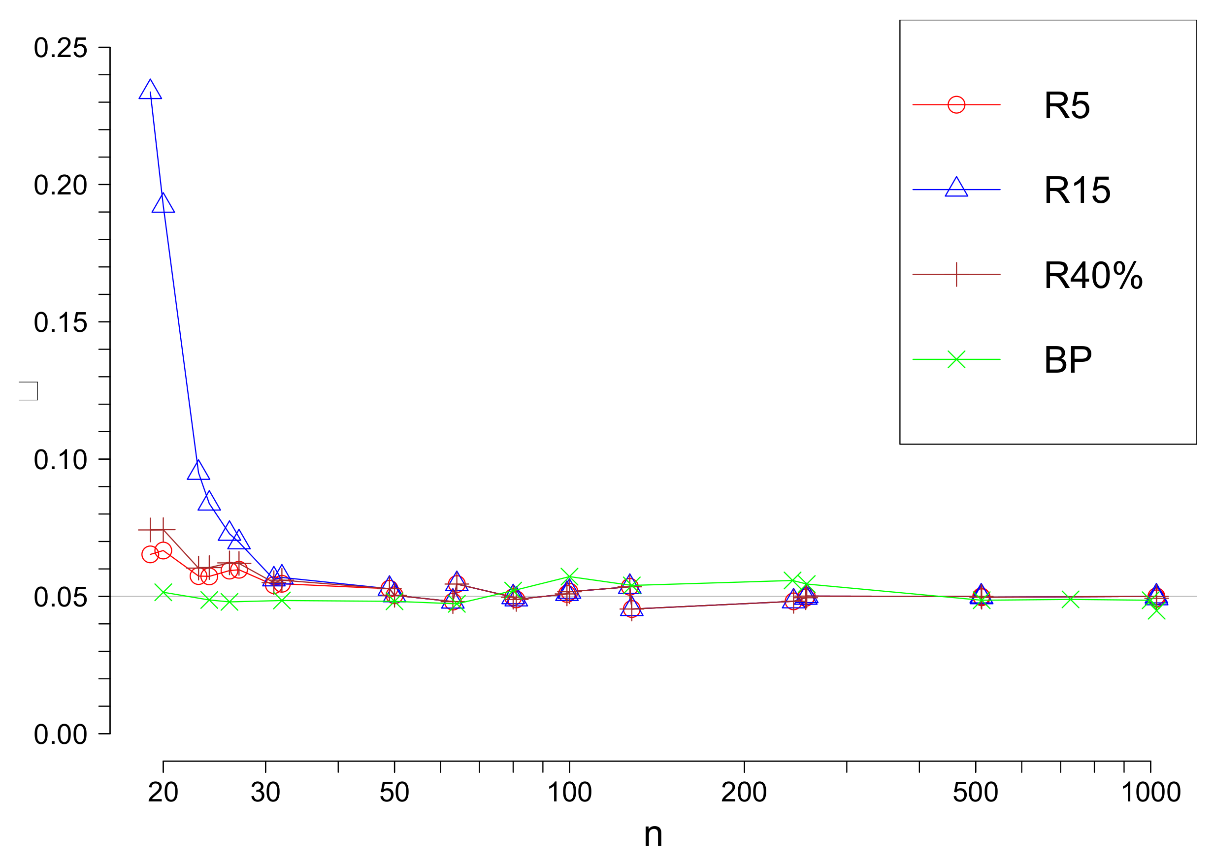
Denote by $R_s$ the Rosner’s test with a fixed upper limit s. Our simulation results confirm that the true significance level is different from the level $\alpha$ suggested by the approximation when n is not large. Nevertheless, it is approaching $\alpha$ as n increases, see Figure 1. The true significance value of the $BP$ test, which uses asymptotic values of the test statistic are also presented in Figure 1.

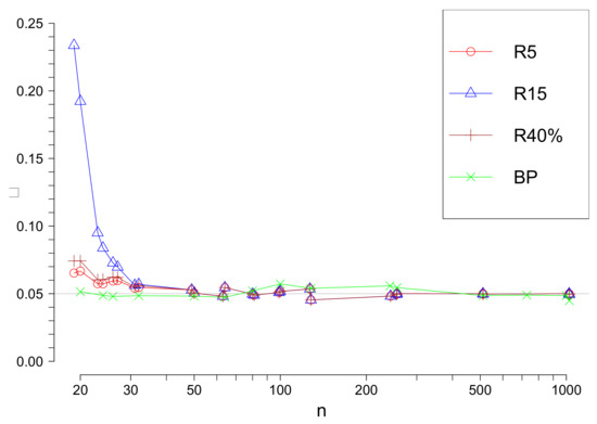
Figure 1. The true values of the significance level of Rosner’s and $BP$ tests in function of n for different values of s ($\alpha =0.05$ is used in approximations).

5.2. Bolshev’s Method

Suppose that the number of contaminants does not exceed s. For $i=1,\cdots ,n$ set

$${\widehat{Y}}_i=(X_i-\overline{X})/s,\hspace{1em}{\tau }_i^{+}=n·(1-T_{n-2}\left({\widehat{Y}}_i\right)),\hspace{1em}{\tau }_i=n·(1-T_{n-2}(|{\widehat{Y}}_i|)),$$

where $\overline{X}$ and s are the empirical mean and standard deviation, $T_{n-2}\left(x\right)$ is the c.d.f. of Thompson’s distribution with $n-2$ degrees of freedom.

Let us consider search for right outliers. Please note that the largest s observations $X_{(n-s+1)},\dots ,X_{\left(n\right)}$ define the smallest s order statistics ${\tau }_{\left(1\right)}^{+}\le \dots \le {\tau }_{\left(n\right)}^{+}$. Possible candidates for outliers are namely the values of $X_{(n-s+1)},\dots ,X_{\left(n\right)}$.

Set ${\tau }^{+}={min}_{1⩽i⩽s}{\tau }_{\left(i\right)}^{+}/i.$

Bolshev’s method for right outliers search. If ${\tau }^{+}\ge {\tau }_{1-\alpha }^{+}(n,s)$, then it is concluded that outliers are absent; here ${\tau }_{1-\alpha }^{+}(n,s)$ is the $1-\alpha$ critical value of the test statistic under ${\mathrm{H}}_0$. If ${\tau }^{+}<{\tau }_{1-\alpha }^{+}(n,s)$, then it is concluded that outliers exist. In such a case outliers are selected in the following way: if ${\tau }_i^{+}/i<{\tau }_{1-\alpha }^{+}(n,s)$ then the value of the order statistic $X_{(n-i+1)}$ is admitted as an outlier, $i=1,\dots ,s$.

In the case of left and right outliers search Bolshev’s method uses ${\tau }_{\left(i\right)}$ instead of ${\tau }_{\left(i\right)}^{+}$, defining the statistic $\tau ={min}_{1⩽i⩽s}{\tau }_{\left(i\right)}/i.$

Bolshev’s method for left and right outliers search. If $\tau \ge {\tau }_{1-\alpha }(n,s)$, then it is concluded that outliers are absent; here ${\tau }_{1-\alpha }(n,s)$ is the $1-\alpha$ critical value of the statistic $\tau$ under ${\mathrm{H}}_0$. If $\tau <{\tau }_{1-\alpha }(n,s)$, then it is concluded that outliers exist. In such a case they are selected in the following way: if ${\tau }_i/i<{\tau }_{1-\alpha }(n,s)$ then the observation corresponding to ${\tau }_i$ is admitted as an outlier, $i=1,\dots ,s$.

5.3. Hawking’s Method

Suppose that the number of contaminants does not exceed s. Let us consider the search for right outliers. For $k=1,\dots ,s$ set

$$b_k^{+}=\frac{1}{\sqrt{k(n-k)}}\sum _{i=1}^k{\tilde{Y}}_{(n-i+1)}=\frac{1}{\sqrt{k(n-k)}}\sum _{i=1}^k(X_{(n-i+1)}-\overline{X})/S_X.$$

$b_k^{+}$ proportional to the sum of k largest ${\tilde{Y}}_{(n-i+1)}$. Set $B^{+}={max}_{1⩽k⩽s}{b}_k^{+}.$

Hawking’s method. If $B^{+}\le B_{\alpha }^{+}(n,s)$ then it is concluded that outliers are absent; here $B_{\alpha }^{+}(n,s)$ is the $\alpha$ critical value of the statistic under ${\mathrm{H}}_0$. If $B^{+}>B_{\alpha }^{+}(n,s)$, then it is concluded that outliers exist. In such a case outliers are selected in the following way: if $b_i^{+}>B_{\alpha }^{+}(n,s)$, then the value of the order statistic $X_{(n-i+1)}$ is admitted as an outlier, $i=1,\dots ,s$.

6. Comparative Analysis of Outlier Identification Methods by Simulation

In the case of location-scale classes probability distribution of all considered test statistics does not depend on $\mu$ and $\sigma$, so we generated samples of various sizes n with $n-r$ observations with the c.d.f. $F_0$ and r observations with various alternative distributions concentrated in the outlier region. We shall call such observations “contaminant outliers”, shortly c-outliers. As was mentioned, outliers which are not c-outliers, i.e., outliers from regular observations with the c.d.f. $F_0$, are very rare.

We repeated simulations $M=$ 100,000 times and using various methods we classified observations to outliers and non-outliers and computed the mean number $D_{O_{c}O}$ of correctly identified c-outliers, the mean number $D_{ON}$ of c-outliers which were not identified, the mean number $D_{NO}$ of non c-outliers admitted as outliers, and the mean number $D_{NN}$ of non c-outliers admitted as non-outliers.

An outlier identification method is ideal if each outlier is detected and each non-outlier is declared as a non-outlier. In practice it is impossible to do with the probability one. Two errors are possible: (a) an outlier is not declared as such (masking effect); (b) a non-outlier is declared as an outlier (swamping effect). We shall write shortly “masking value” for the mean number of non-detected c-outliers and “swamping value” for the mean number of “normal” observations declared as outliers in the simulated samples.

If swamping is small for two tests then a test with smaller masking effect should be preferred because in this case the distribution of the data remaining after excluding of suspected outliers should be closer to the distribution of non-outlier data.

From the other side, if swamping for Method 1 is considerably bigger than swamping of Method 2 and masking is smaller for Method 1, then it does not mean that Method 1 is better because this method rejects many extreme non-outliers from the tails of the regular distribution $F_0$ and the sample remaining after classification may be not treated as a sample from this regular distribution even if all c-outliers are eliminated.

For various families of distributions, sample sizes n, and alternatives we compared Davies-Gather ($DG$) and new ($BP$) methods performance. In the case of normal distribution we also compared them with Rosner’s, Bolshev’s and Hawking’s methods.

We used two different classes of alternatives: in the first case c-outliers are spread widely in the outlier region around the mean, in the second case c-outliers are concentrated in a very short interval laying in the outlier region. More precisely, if right outliers were searched, then we simulated r observations concentrated in in the right outlier region $ou{t}_r({\alpha }_n,F_0)=\{x:x>x_{{\alpha }_n}\}$ using the following alternative families of distribution:

(1)

Two parameter exponential distribution $\mathcal{E}(\theta ,x_{{\alpha }_n})$ with the scale parameter $\theta$. If $\theta$ is small, then outliers are concentrated near the border of the outlier region. If $\theta$ is large then outliers are widely spread in the outlier region. If $\theta$ increases, then the mean of outlier distribution increases. Please note that even if $\theta$ is very near 0 and the true number of outliers r is large, these outliers may corrupt strongly the data making tails of histogram two heavy.

(2)

Truncated normal distribution $\mathcal{T}\mathcal{N}(x_{{\alpha }_n},\mu ,\rho )$ with the location and scale parameters $\mu ,\rho$ ($\mu >x_{{\alpha }_n})$. If $\rho$ is small then this distribution is concentrated in a small interval around $\mu$. If $\mu$ increases, then the mean of outlier distribution increases.

For lack of place we present a small part of our investigations. Please note that the results are very similar for all sample sizes $n\ge 20$. Multiple outlier problem is not very relevant for smaller sample sizes.

6.1. Investigation of Outlier Identification Methods for Normal Data

We use notation $B,H,R,DG$, and $BP$ for the Bolshev’s, Hawking’s, Rosner’s, Davies-Gather’s, and the new methods, respectively. If $DG$ method is based on maximum likelihood estimators, then we write $D{G}_{ml}$ method, if it is based on robust estimators, we write $D{H}_{rob}$ method.

For comparison of above considered methods we fixed the significance level $\alpha =0.05$. We remind that the significance level $\alpha$ is the probability to reject minimum one observation as an outlier under the hypothesis ${\mathrm{H}}_0$ which means that all observations are realizations of i.i.d. with the same normal distribution. The only test, namely R method uses approximate critical values of the test statistic, so the significance values for this test is only approximately $0.05$ and depends on s and n. In Figure 1 the true significance level value for $s=5,15$ and $\left[0.4n\right]$ in function of n are given.

The $B,H$, and R tests methods have a drawback that the upper bound for the possible number of outliers s must be fixed. The $BP$ and $DG$ tests have an advantage that they do not require it.

Our investigations showed that H,B and $D{G}_{ml}$ methods have other serious drawbacks. So firstly let us look closer at these methods.

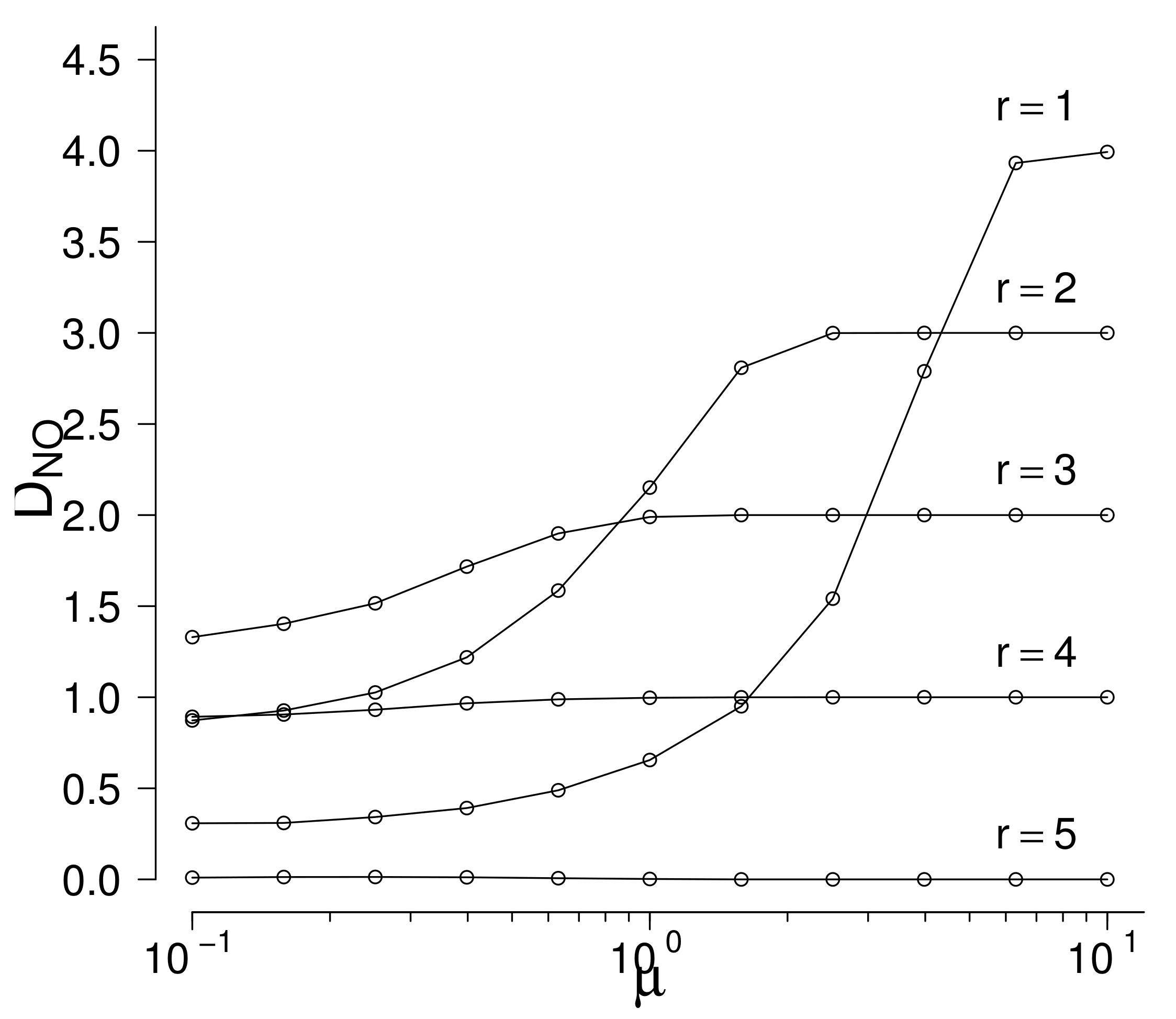
If the true number of c-outliers r exceeds s, then the B and H methods cannot find them even if they are very far from the limits of the outlier region. Nevertheless, suppose that r does not exceed s and look at the performance of the H method. Set $n=100$, $s=5$, and suppose that c-outliers are generated by right-truncated normal distribution $\mathcal{T}\mathcal{N}(x_{{\alpha }_n},\mu ,\rho )$ with fixed $\rho$ and increasing $\mu$. Note that the true number of c-outliers is supposed to be unknown but do not exceed $s=5$. In Figure 2 the mean numbers of rejected non-c-outliers $D_{NO}$ are given in function of the parameter $\mu$ (the value of the parameter $\rho =0.1^2$ is fixed) for fixed values of r see Figure 2. In Table 7 the values of $D_{NO}$ plus the values of the mean numbers of truly rejected c-outliers are given. Table 7 shows that if $r=1$, then if $\mu$ is sufficiently large, the c-outlier is found but the number of rejected non-c-outliers $D_{NO}$ increases to 4, so swamping is very large. Similarly, if $r=2$, then $D_{NO}$ increases to 3, so swamping is large. Beginning from $r=3$ not all c-outliers are found even for large $\mu$. Swamping is smallest if the true value r coincides with s but even in this case one c-outlier is not found even for large $\mu$. Taking into account that the true number r of c-outliers is not known in real data, the performance of the H methos is very poor. Results are similar for other values of n, s, and distributions of c-outliers. As a rule, H mehod finds rather well the c-outliers but swamping is very large because this method has a tendency to reject a number near s of observations for remote alternatives. which is good if $r=s$ but is bad if r is different from s.

Figure 2. Hawkin’s method: the values of $D_{NO}+D_{OO}$ in function of $\mu$ and r ($n=100$, $s=5$).

Table 7. Hawkin’s method: the values of $D_{NO}+D_{OO}$ in function of $\mu$ and r ($n=100$, $s=5$).

r \ $\mathit{\mu }$	0.1	1	6.3	10
1	0.31 + 0.00	0.66 + 0.00	3.93 + 1.00	3.99 + 1.00
2	0.87 + 0.00	2.15 + 0.06	3.00 + 1.21	3.00 + 2.00
3	1.33 + 0.08	1.99 + 0.84	2.00 + 2.00	2.00 + 2.00
4	0.89 + 0.58	1.00 + 1.42	1.00 + 3.00	1.00 + 3.00
5	0.01 + 1.15	0.00 + 2.03	0.00 + 3.02	0.00 + 3.96

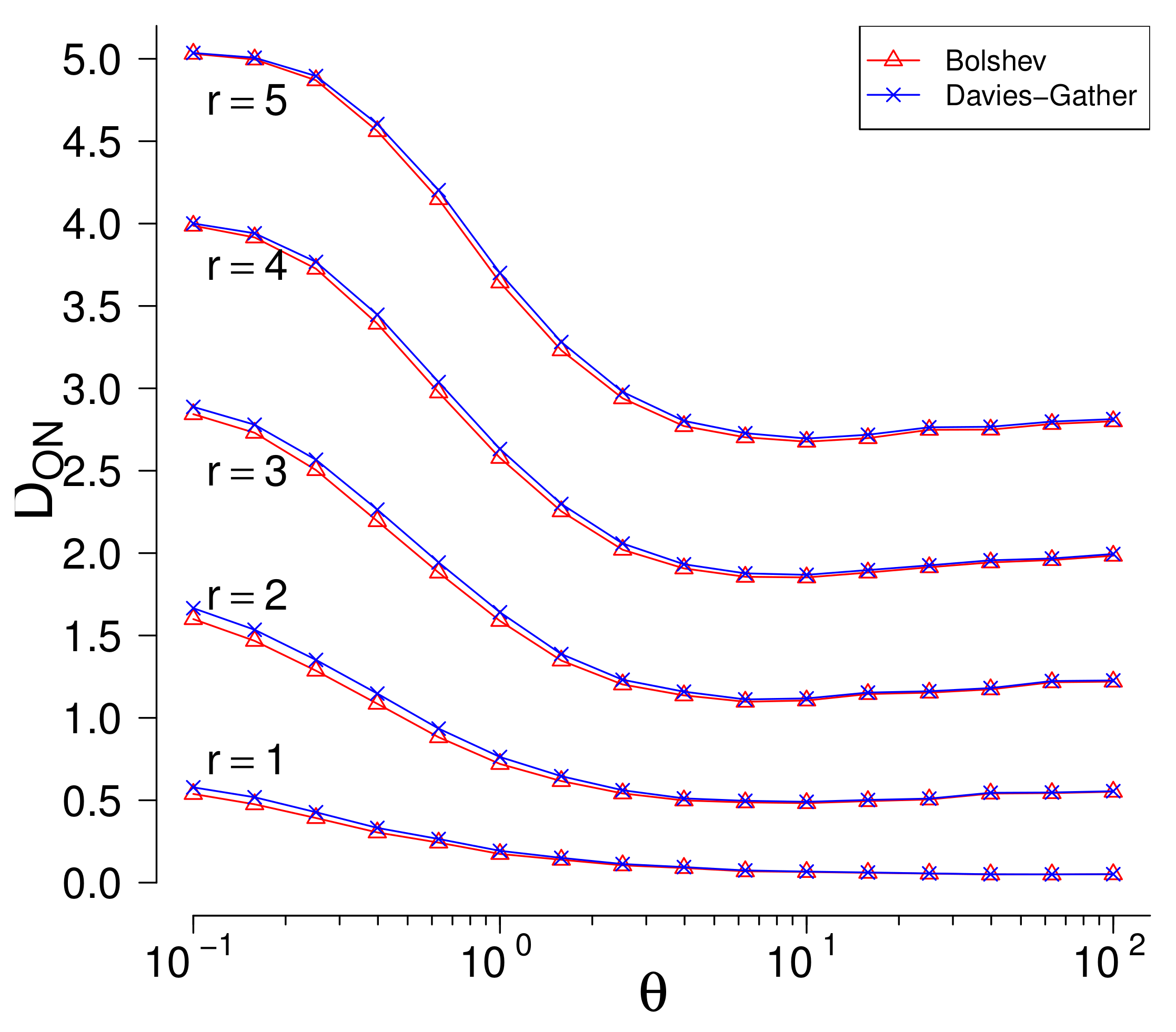
The B and $D{G}_{ml}$ tests have a drawback that they use maximum likelihood estimators which are not robust and estimate parameters badly in presence of outliers. Once more, set $n=100$, $s=5$, and suppose that c-outliers are generated by two-parameters exponential distribution $\mathcal{T}\mathcal{E}(x_{{\alpha }_n},\theta )$ with increasing $\theta$. Swamping values are negligible in, so only masking values( mean numbers of non-rejected c-outliers $D_{ON}$) are important. In Figure 3 the masking values in function of the parameter $\theta$ are given for fixed values of r.

Figure 3. The number of outliers rejected as non-outliers ($D_{ON}$). The alternative: two-sided, the outliers generated by two-parameters exponential distribution on both sides.

Both methods perform very similarly. The masking values are large for every value of $r>1$. If r increases, then masking values increase, too. For example, if $r=5$, then almost 3 c-outliers from 5 are not rejected on average even for large values of $\theta$.

Similar results hold taking other values of n, s and various distributions of c-outliers.

The above analysis shows that the B, H, $D{G}_{ml}$ methods have serious drawbacks, so we exclude these methods from further consideration.

Let us consider the remaining three methods: R, $DG$, and $BP$. For small n the true significance level of Rosner’s test differ considerably from the suggested, so we present comparisons of tests performance for $n=50,100,1000$ (see Table 8 and Table 9). Truncated exponential distribution was used for outliers simulation. Remoteness of the mean of outliers from the border of the outlier region is characterized by the parameter $\theta$.

Table 8. The masking values $D_{ON}$ ($n=50$ and $n=100$).

	$\mathit{n}=50$							$\mathit{n}=100$
r	Method$\backslash \mathbf{\theta }$	0.1	0.4	1	4	10	r	0.1	0.4	1	4	10
2	$Rosne{r}_5$	1.36	0.95	0.51	0.15	0.06	2	1.19	0.71	0.33	0.09	0.04
	$Rosne{r}_{15}$	1.36	0.95	0.51	0.15	0.06		1.19	0.71	0.33	0.09	0.04
	$Rosne{r}_{\left[0.4n\right]}$	1.36	0.95	0.51	0.15	0.06		1.19	0.71	0.33	0.09	0.04
	$DG{r}_{rob}$	1.56	1.17	0.71	0.24	0.10		1.31	0.84	0.44	0.13	0.06
	$BP$	0.92	0.66	0.37	0.10	0.04		0.50	0.32	0.15	0.04	0.02
5	$Rosne{r}_5$	3.79	3.31	2.11	0.48	0.16	5	3.52	2.57	1.27	0.27	0.10
	$Rosne{r}_{15}$	3.66	3.21	2.04	0.46	0.16		3.43	2.52	1.24	0.26	0.10
	$Rosne{r}_{\left[0.4n\right]}$	3.66	3.21	2.04	0.46	0.16		3.43	2.52	1.24	0.26	0.10
	$D{G}_{rob}$	4.70	4.10	2.90	1.09	0.48		4.23	3.01	1.81	0.57	0.25
	$BP$	2.00	1.68	1.18	0.40	0.15		0.78	0.60	0.43	0.15	0.07
8	$Rosne{r}_5$	8.00	7.97	7.54	3.70	3.06	10	10.0	9.90	8.21	5.10	5.00
	$Rosne{r}_{15}$	5.70	5.48	4.52	1.00	0.29		6.88	6.54	4.36	0.69	0.22
	$Rosne{r}_{\left[0.4n\right]}$	5.70	5.48	4.52	1.00	0.29		6.88	6.54	4.36	0.69	0.22
	$D{G}_{rob}$	7.90	7.49	6.10	2.67	1.24		9.74	8.38	5.78	2.12	0.92
	$BP$	4.27	3.84	3.25	1.47	0.57		2.21	1.90	1.73	0.74	0.30

Table 9. The masking values $D_{ON}$ ($n=1000$).

r	Method $\backslash \mathit{\theta }$	0.1	0.4	1	4	1000
5	$Rosne{r}_5$	2.15	0.69	0.29	0.07	0.00
	$Rosne{r}_{15}$	2.12	0.66	0.27	0.07	0.00
	$Rosne{r}_{\left[0.4n\right]}$	2.12	0.66	0.27	0.07	0.00
	$D{G}_{rob}$	1.99	0.78	0.35	0.09	0.00
	$BP$	0.25	0.23	0.22	0.11	0.00
20	$Rosne{r}_5$	19.0	15.8	15.0	15.0	15.0
	$Rosne{r}_{15}$	19.2	10.9	5.52	5.00	5.00
	$Rosne{r}_{\left[0.4n\right]}$	12.7	6.94	1.76	0.30	0.00
	$D{G}_{rob}$	14.8	6.97	3.32	1.93	0.00
	$BP$	0.29	0.26	0.23	0.18	0.00
100	$Rosne{r}_5$	100	99.9	96.7	95.0	95.0
	$Rosne{r}_{15}$	100	99.92	96.4	85.0	85.0
	$Rosne{r}_{\left[0.4n\right]}$	55.8	56.8	50.4	4.43	0.01
	$D{G}_{rob}$	100	89.9	61.6	22.2	0.1
	$BP$	4.72	4.00	3.95	3.58	0.04

Swamping values $D_{NO}$ (the mean numbers of non-c-outliers declared as outliers) are very small for all tests. For example, even if $n=1000$, the R and $DG$ methods reject on average as outliers only 0.05 from $n-r=995,980,900$ non-c-outliers. For the $BP$ method this number is $0.25,0.19,0.05$ from $995,980$, and 900 non-c-outliers, respectively. So only masking values $D_{ON}$ (the mean numbers of c-outliers declared as non-outliers) are important for outlier identification methods comparison.

Necessity to guess the upper limit s for a possible number of outliers is considered as a drawback of the Rosner’s method. Indeed, if the true number of outliers r is greater than the chosen upper limit s, then $r-s$ outliers are not identified with the probability one. In addition, even if $r\le s$, it is not clear how important is closeness of r to s. So first we investigated the problem of the upper limit choice.

Here we present masking values $D_{ON}$ of the Rosner’s tests for $s=5,15$ and $\left[0.4n\right]$. Similar results are obtained for other values of s.

Our investigations show that it is sufficient to fix $s=\left[0.4n\right]$, which is clearly larger than it can be expected in real data. Indeed, Table 8 and Table 9 show that for $r>s$$Rosne{r}_5$ and $Rosne{r}_{15}$ do not find $r-s$ outliers even if they are very remote, as it should be. Nevertheless, we see that even if the true number of outliers r is much smaller than $\left[0.4n\right]$, for any considered n, $r\le s=5,15$ the masking values of the $Rosne{r}_{\left[0.4n\right]}$ test are approximately the same (even a little smaller) as the masking values of the tests $Rosne{r}_5$ and $Rosne{r}_{15}$, for $r>s$ they are clearly smaller.

Hence, $s=\left[0.4n\right]$ should be recommended for Rosner’s test application, and performance of $Rosne{r}_{\left[0.4\right]}$, Davies-Gather robust ($D{G}_{rob})$ and the proposed $BP$ methods should be compared.

All three methods find all c-outliers if they are sufficiently remote. For $n=50$ the $BP$ method gives uniformly smallest masking values and the $DG$ method gives uniformly largest masking values for any considered r in all diapason of alternatives. For $n=100$ and $r=2,5$ the result is the same. For $n=100$ and $r=10$ (it means that even for very small $\theta$ the data is seriously corrupted) the BP method is also the best except that for the most remote alternatives the $Rosne{r}_{\left[0.4n\right]}$ method slightly outperforms the BP method. For $n=1000$ and the most of alternatives the BP method strongly outperforms other methods, except the most remote alternatives.

The $DG$ and Rosner’s methods have very large masking if many outliers are concentrated near the outlier region border. In this case data is seriously corrupted; however, these methods do not see outliers.

Conclusion: in most considered situations the $BP$ method is the best outlier identification method. The second is Rosner’s method with $s=\left[0.4\right]$, and the third is the Davies-Gather method based on robust estimation. Other methods have poor performance.

6.2. Investigation of Outlier Identification Methods for Other Location-Scale Models

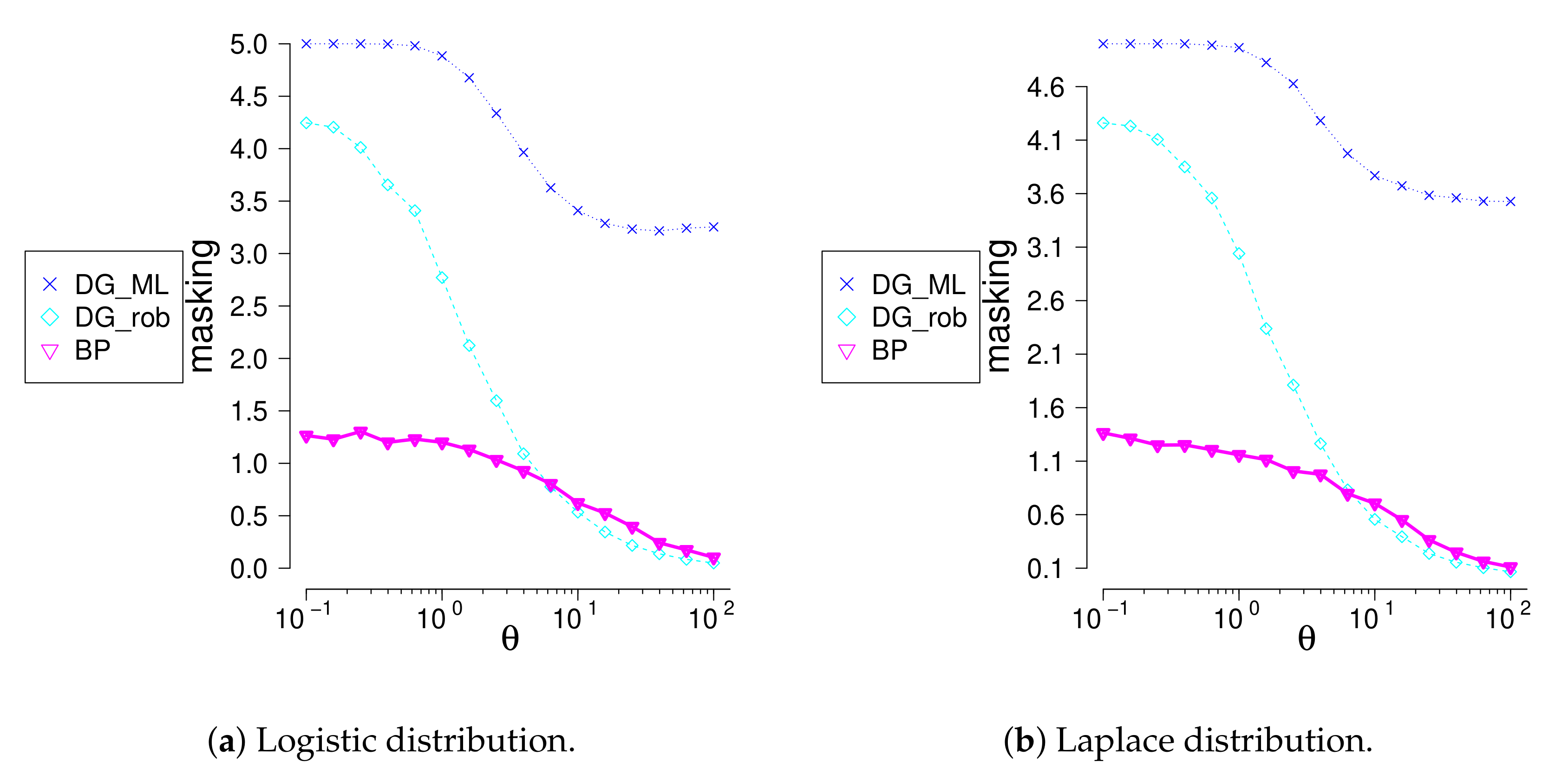
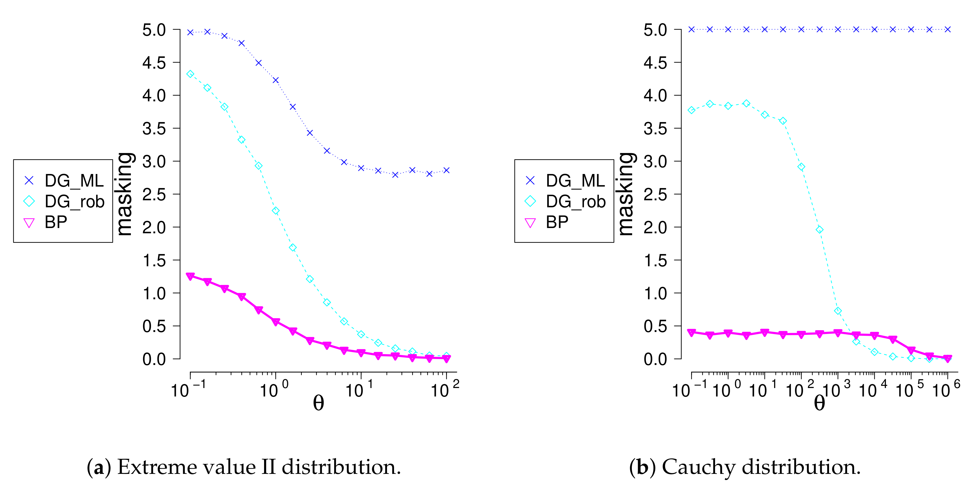
We investigated performance of the new method for location-scale families different from normal. We compare the $BP$ method with the generalized Davies-Gather method for logistic, Laplace (symmetric, $F\in {\mathcal{G}}_0\cap {\mathcal{F}}_{ls}$), extreme values (non-symmetric $F\in {\mathcal{G}}_0\cap {\mathcal{F}}_{ls}$), and Cauchy (symmetric, $F\in {\mathcal{G}}_1\cap {\mathcal{F}}_{ls}$) families. C-outliers were generating using truncated exponential distribution concentrated in two-sided outlier region. Swamping values being small, masking value, see Table 10 and differences between the true number of c-outliers and the number of rejected observations, see Figure 4 and Figure 5, were compared. The $BP$ and $D{G}_{rob}$ methods find very well the most remote outliers; meanwhile, the $BP$ method identifies much better closer outliers. The $D{G}_{rob}$ method identifies badly multiple outliers concentrated near the border of the outlier region, whereas the $BP$ method does well. The $D{G}_{ML}$ is not appropriate for multiple outlier search.

Table 10. Masking values for logistic, Laplace, extreme value II and Cauchy distribution, when $n=100$, $r=5$.

	Logistic				Laplace
Method$\backslash \mathbf{\theta }$	0.1	1	6.3	10	0.1	1	6.3	10
$D{G}_{ML}$	5	4.89	3.64	3.42	5	4.96	3.98	3.78
$D{G}_{rob}$	4.21	2.69	0.76	0.51	4.27	2.98	0.87	0.59
$BP$	1.3	1.13	0.78	0.64	1.31	1.21	0.8	0.66
	Extreme Value II				Cauchy
Method$\backslash \mathbf{\theta }$	0.1	1	6.3	10	1	100	1000	${\mathbf{10}}^{\mathbf{5}}$
$D{G}_{ML}$	4.96	4.19	3	2.9	5	5	5	5
$D{G}_{rob}$	4.29	2.25	0.59	0.4	3.81	2.89	0.8	0.01
$BP$	1.25	0.56	0.14	0.11	0.38	0.4	0.39	0.13

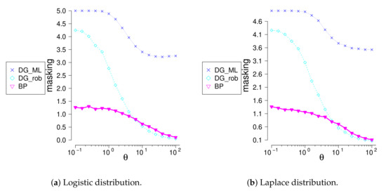
Figure 4. The difference between number outliers and rejected observations given that sample size $n=100$ and $r=10$ outliers.

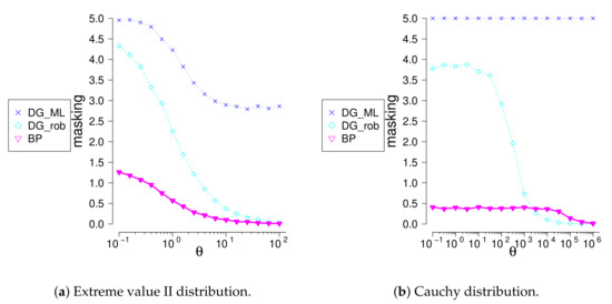
Figure 5. The difference between number outliers and rejected observations given that sample size $n=100$ and $r=10$ outliers.

7. Conclusions

We compared by simulation outlier identification results of the new method and methods given in previous studies. Even in the case of the normal model, which is investigated by many authors, the new method shows excellent identification power. In many situations, it has superior performance as compared to existing methods.

The obtained results widened considerably the spectre of most used non-regression models needing outlier identification methods. Many two-parameter models such as Weibull, logistic and loglogistic, extreme values, Cauchy, Laplace, and others can be investigated applying the new method.

The advantage of the proposed outlier identification method is that it has very good potential for generalizations. The authors are at the completion stage of research on outlier identification methods for accelerated failure time regression models and generalized linear models, gamma regression model in particular. Outlier identification methods for time series is another direction of the future work. Possible direction is investigation of Gaussian mixture regression models (see [29]).

Limitation of the new method is that it cannot be applied for analysis of discreet models. Taking into consideration that the method is based on asymptotic results, we recommend not applying it to samples of very small size $n\le 15$.

The R package outliersTests was created for the practical usage of proposed test.

References

- Bol’shev, L.; Ubaidullaeva, M. Chauvenet’s Test in the Classical Theory of Errors. Theory Probab. Appl. 1975, 19, 683–692. [Google Scholar] [CrossRef]
- Davies, L.; Gather, U. The Identification of Multiple Outliers. J. Am. Stat. Assoc. 1993, 88, 782–792. [Google Scholar] [CrossRef]
- Dixon, W.J. Analysis of Extreme Values. Ann. Math. Stat. 1950, 21, 488–506. [Google Scholar] [CrossRef]
- Grubbs, F.E. Sample Criteria for Testing Outlying Observations. Ann. Math. Stat. 1950, 21, 27–58. [Google Scholar] [CrossRef]
- Rosner, B. On the Detection of Many Outliers. Technometrics 1975, 17, 221–227. [Google Scholar] [CrossRef]
- Tietjen, G.L.; Moore, R.H. Some Grubbs-Type Statistics for the Detection of Several Outliers. Technometrics 1972, 14, 583–597. [Google Scholar] [CrossRef]
- Barnett, V.; Lewis, T. Outliers in Statistical Data; John Wiley & Sons: Hoboken, NJ, USA, 1974. [Google Scholar]
- Zerbet, A. Statistical Tests for Normal Family in Presence of Outlying Observations. In Goodness-of-Fit Tests and Model Validity; Huber-Carol, C., Balakrishnan, N., Nikulin, M.S., Mesbah, M., Eds.; Birkhäuser Boston: Basel, Switzerland, 2002; pp. 57–64. [Google Scholar]
- Chikkagoudar, M.; Kunchur, S.H. Distributions of test statistics for multiple outliers in exponential samples. Commun. Stat. Theory Methods 1983, 12, 2127–2142. [Google Scholar] [CrossRef]
- Kabe, D.G. Testing outliers from an exponential population. Metrika 1970, 15, 15–18. [Google Scholar] [CrossRef]
- Kimber, A. Testing upper and lower outlier paris in gamma samples. Commun. Stat. Simul. Comput. 1988, 17, 1055–1072. [Google Scholar] [CrossRef]
- Lalitha, S.; Kumar, N. Multiple outlier test for upper outliers in an exponential sample. J. Appl. Stat. 2012, 39, 1323–1330. [Google Scholar] [CrossRef]
- Lewis, T.; Fieller, N.R.J. A Recursive Algorithm for Null Distributions for Outliers: I. Gamma Samples. Technometrics 1979, 21, 371–376. [Google Scholar] [CrossRef]
- Likeš, I.J. Distribution of Dixon’s statistics in the case of an exponential population. Metrika 1967, 11, 46–54. [Google Scholar] [CrossRef]
- Lin, C.T.; Balakrishnan, N. Exact computation of the null distribution of a test for multiple outliers in an exponential sample. Comput. Stat. Data Anal. 2009, 53, 3281–3290. [Google Scholar] [CrossRef]
- Lin, C.T.; Balakrishnan, N. Tests for Multiple Outliers in an Exponential Sample. Commun. Stat. Simul. Comput. 2014, 43, 706–722. [Google Scholar] [CrossRef]
- Zerbet, A.; Nikulin, M. A new statistic for detecting outliers in exponential case. Commun. Stat. Theory Methods 2003, 32, 573–583. [Google Scholar] [CrossRef]
- Torres, J.M.; Pastor Pérez, J.; Sancho Val, J.; McNabola, A.; Martínez Comesaña, M.; Gallagher, J. A functional data analysis approach for the detection of air pollution episodes and outliers: A case study in Dublin, Ireland. Mathematics 2020, 8, 225. [Google Scholar] [CrossRef]
- Gaddam, A.; Wilkin, T.; Angelova, M.; Gaddam, J. Detecting Sensor Faults, Anomalies and Outliers in the Internet of Things: A Survey on the Challenges and Solutions. Electronics 2020, 9, 511. [Google Scholar] [CrossRef]
- Ferrari, E.; Bosco, P.; Calderoni, S.; Oliva, P.; Palumbo, L.; Spera, G.; Fantacci, M.E.; Retico, A. Dealing with confounders and outliers in classification medical studies: The Autism Spectrum Disorders case study. Artif. Intell. Med. 2020, 108, 101926. [Google Scholar] [CrossRef]
- Zhang, C.; Xiao, X.; Wu, C. Medical Fraud and Abuse Detection System Based on Machine Learning. Int. J. Environ. Res. Public Health 2020, 17, 7265. [Google Scholar] [CrossRef] [PubMed]
- Souza, T.I.; Aquino, A.L.; Gomes, D.G. A method to detect data outliers from smart urban spaces via tensor analysis. Future Gener. Comput. Syst. 2019, 92, 290–301. [Google Scholar] [CrossRef]
- Hawkins, D.M. Identification of Outliers; Springer: Dordrecht, The Netherlands, 1980; Volume 11. [Google Scholar]
- Kimber, A.C. Tests for Many Outliers in an Exponential Sample. J. R. Stat. Soc. 1982, 31, 263–271. [Google Scholar] [CrossRef]
- De Haan, L.; Ferreira, A. Extreme Value Theory: An Introduction; Springer: New York, NY, USA, 2007. [Google Scholar]
- Rousseeuw, P.J.; Croux, C. Alternatives to the median absolute deviation. J. Am. Stat. Assoc. 1993, 88, 1273–1283. [Google Scholar] [CrossRef]
- Liu, Y.; Abeyratne, A.I. Practical Applications of Bayesian Reliability; John Wiley & Sons: Hoboken, NJ, USA, 2019. [Google Scholar]
- Rosner, B. Percentage points for the RST many outlier procedure. Technometrics 1977, 19, 307–312. [Google Scholar] [CrossRef]
- Su, H.; Hu, Y.; Karimi, H.R.; Knoll, A.; Ferrigno, G.; De Momi, E. Improved recurrent neural network-based manipulator control with remote center of motion constraints: Experimental results. Neural Netw. 2020, 131, 291–299. [Google Scholar] [CrossRef] [PubMed]
Publisher’s Note: MDPI stays neutral with regard to jurisdictional claims in published maps and institutional affiliations. |
© 2020 by the authors. Licensee MDPI, Basel, Switzerland. This article is an open access article distributed under the terms and conditions of the Creative Commons Attribution (CC BY) license (http://creativecommons.org/licenses/by/4.0/).