1. Introduction
Statistical methods for meta-analysis have been widely applied in many research areas and are of particular importance in healthcare studies. When randomised controlled clinical trials (or studies) are made of a medical treatment for patients with a given disease and heterogeneous samples are compiled, a meta-analysis may be conducted to determine what can fairly be concluded about the fundamental question addressed in each such study, i.e., the effectiveness of the treatment. This parameter is usually estimated on the basis of a prior estimate of the between-study variation, for which purposes random-effects meta-analysis techniques are employed. Thus, meta-analysis addresses the problem of drawing inferences concerning the treatment effect based on
k samples. Between-sample heterogeneity introduces additional uncertainty into the process, namely that of model uncertainty. Rücker et al. [
1] commented that statistical heterogeneity and small study effects are major issues affecting the validity of meta-analysis. Heterogeneity is difficult to estimate if few studies are considered, and the resulting model uncertainty might lead to misleading results being obtained. In this paper, we define heterogeneity as the statistical variation found in the collected effect size data, which has to be assessed after the studies have been pooled [
1].
According to Sutton and Abrams [
2], the Bayesian random-effects model for meta-analyses is given by:
where for each study
the observed effect
is assumed to be normally distributed with mean parameter
(the treatment effectiveness conditional on study
i) and variance
. Similarly,
represents the unconditional treatment effectiveness, i.e., the pooled effect size;
is its variance; and
indicates a prior density to be assigned. When the effectiveness is measured by a discrete 0–1 random variable, the above hierarchical normal model is typically applied to the logit transformation of the data
with the reparametrisation
[
3,
4,
5,
6,
7,
8]. If the samples contain zeros, a fixed data continuity correction is applied, and a logit approximation is then used. However, this practice has been criticised by Sweeting et al. [
9], who proposed an alternative empirical data correction. Furthermore, small studies present more heterogeneity than large ones [
10]. Recently, Weber et al. (2020) [
11] recommended that zero-cell corrections should be avoided due to the poor performance of their statistical properties. Obviously, continuity corrections are not the only way to proceed. A number of meta-analysis methods based, e.g., on binomial models were proposed in [
12] and the references therein.
In the meta-analysis literature, determining statistical heterogeneity mainly consists of either estimating the between-study variation, characterised as the variance, or heterogeneity parameter, or otherwise testing the null hypothesis that the true treatment effects across studies are identical
[
8,
13]. A measure of evidence for heterogeneity is obtained by means of the
Q test, a chi-squared test with
degrees of freedom, first defined by Cochran [
14]. Alternatively, and in order to overcome the dependence on the number of studies considered for the meta-analysis, which is the case with the
Q test, Higgings and Thompson [
15] proposed the dimensionless
index, which describes the percentage of variation across studies that is due to heterogeneity rather than chance. Mittlböck and Heinzl [
16] compared these two relative measures of heterogeneity jointly with the index
through an intensive simulation study. Basically,
and
have similar properties, although
is preferred when few studies are considered. As shown in [
16], the number of studies affects the power of the heterogeneity test and the heterogeneity measures
, but not
.
It is well known that all tests of heterogeneity have relatively little power to detect heterogeneity when data are sparse and/or when meta-analyses are based on a small number of studies [
1,
9,
15,
17]. These situations are very common in daily practice, for instance with respect to rare or orphan diseases, where zero values are often observed in both the trial and the treatment arms considered.
Statistical heterogeneity is a characteristic of the studies that compose a meta-analysis and can be present at different levels of intensity, ranging from homogeneity to heterogeneity. There are also many intermediate situations that should be considered in order to correctly estimate the quantities of interest. Higgins et al. [
18] proposed a tentative naive categorisation of values for
, relating values of
,
and
with low, moderate and high levels of heterogeneity, respectively, and considering a significant degree of heterogeneity to be present when
In the present analysis, we address the question from a different standpoint, arguing that between-sample heterogeneity is a clustering problem and that model uncertainty can be incorporated into the inference using a Bayesian procedure. Under this procedure, the posterior probabilities of the cluster models are computed, and the meta-inference is then obtained as a mixture of the meta-inferences obtained for the cluster models, using the posterior model probabilities as a mixing distribution. Another point of difference is that most previous studies analysed between-study heterogeneity for a quantity of interest in the comparison of two treatments, such as the mean difference, relative risk or odds ratio. In our proposal, the configuration of between-study heterogeneity is analysed for each treatment separately, which allows the heterogeneity structure to differ between the experimental treatment and the control.
The proposed methodology is known as Bayesian model averaging and has recently begun to be used in meta-analyses. For instance, Bayesian meta-analyses modelling averages over fixed and random effect models were considered in Gronau et al. [
19] and Scheibehenne et al. [
20].
1.1. A Motivating Example
Günhan et al. [
12] suggested the use of weakly informative priors for the treatment effect parameter of a Bayesian meta-analysis model, to be applied in a paediatric transplant dataset. In the present study, and for illustrative purposes, we focus on a dataset corresponding to renal post-transplant lymphoproliferative diseases (PTLD). The results obtained are shown in
Table 1.
In this respect, Crins et al. [
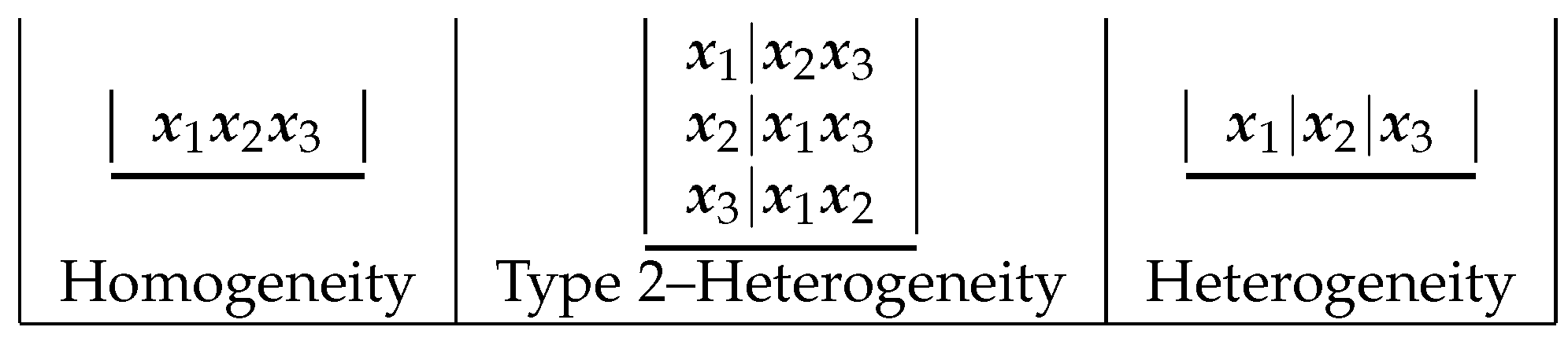
21] conducted Cochrane’s Q test and found no evidence of heterogeneity between the trials. Moreover, Günhan et al. obtained low values for the estimated heterogeneity parameter under weakly informative or vague priors and maximum likelihood estimation. However, the structure of the partition clustering induced by the PTLD dataset in
Table 1 shown in
Figure 1 indicates that different forms of inter-trial variability could be present.
There are possible partitions (models or heterogeneity configurations), and for each of the cluster classes, there are partitions, respectively. Thus, the selection of any one model (homogeneity, for example) among the five that are possible may ignore the uncertainty underlying model selection and misrepresent the uncertainty concerning the quantities of interest. In view of these considerations, we believe that Bayesian model averaging (BMA) is an appropriate means of accounting for model uncertainty and, thus, heterogeneity. Expectations and quantities of interest are obtained by weighted averages over the set of models, rather than by selecting a single model and drawing inferences as if it were the true model.
For each of the treatments considered (control and experimental),
Table 2 shows the (posterior) probabilities of each of the five models induced by the clustering applied to the data in this example. These posterior probabilities constitute the weights to be used for averaging the set of models. Their expressions are given in
Section 3. As an example, let us observe the control treatment. The case of homogeneity has the highest posterior probability of being true, 0.39. However, this option does not consider the remaining heterogeneity structures and therefore would result in misleading inferences being drawn, by rejecting all other possible models, which constitute a combined probability of 0.61. The same reasoning is applicable to the experimental treatment.
The BMA approach to meta-analysis involves averaging over all the possible models when making inferences about the quantities of interest. For example, for the dataset considered in this case study, if
is the treatment effect under the control treatment, its posterior distribution, for the data given, is:
i.e., the average of the posterior distributions under each of the models (“type of heterogeneity”) considered, weighted by its posterior model probability. For instance, the posterior mean for
is a weighted average of the posterior means in each model:
where the posterior probability for model
can be obtained by:
where:
is the integrated likelihood of the model
,
is the vector of the parameters of model
,
is the prior density of
under model
is the likelihood and
is the prior probability of model
All probabilities are implicitly conditional on
the set of all models being considered, where
represents its cardinal.
1.2. Summary
The rest of this paper is organised as follows. The binomial Bayesian models and the conditional distributions linking the experimental parameters
and the meta-parameter
are presented in
Section 2, where the Bayesian procedure for clustering the samples and the likelihood of the meta-parameter are also given. The Bayesian model averaging procedure for estimating the meta-parameters is described in
Section 3. Three illustrative examples are provided in the following section, with real datasets. Finally,
Section 5 summarises the main conclusions drawn and presents some concluding remarks.
2. The Bayesian Binomial Model
Assume a meta-analysis involves
k studies that provide
k independent discrete samples with the binomial distribution
, where
represents the treatment effectiveness,
the number of patients and
the number of successful treatments, conditional on the study
i. Assume, moreover, that the prior information on the conditional treatment effectiveness
is weak. Accordingly, the uniform prior
is used in a context where the data contain zeros [
22,
23]. Therefore, for
, we consider the Bayesian sampling models:
where:
and
is the indicator function. The value of one is assigned to all elements of
A, and zero elsewhere. In this analysis, it is convenient to consider a
latent variable
x, the meta-variable, which is defined as the result obtained when a treatment with meta-effectiveness
is applied to a patient in a virtual study, which is not affected by between-study variability. The distribution of this meta-variable
x is of the same type as that of
, and hence, we have the Bernoulli meta-model
, where the meta-parameter
represents the true (unconditional) treatment effect. This meta-model gives a precise meaning to the meta-parameter
. The objective Bayesian meta-model
M is then given by:
The Bayesian meta-analysis is then based on the posterior distribution of the parameter
which is given by:
where
The likelihood function in (
9) cannot be obtained with the information on sample
on study
i, which is related to
, but not to
. Therefore, further steps are required to derive an appropriate likelihood function for
:
A distribution is needed to link the experimental parameters and the meta-parameter This linking distribution must ensure there is coherence between the conditional and marginal distributions of the experimental parameter and the meta-parameter. Mathematically, this requires that the corresponding bivariate distribution belong to the class of bivariate distributions with given marginals.
It is clear that the likelihood of strongly depends on the cluster structure of the samples. Therefore, before formulating the likelihood of for the samples , we must address the important question of whether k, the dimension of the model, can be reduced by clustering homogeneous samples.
In other words, each cluster model indicates a different heterogeneity structure of the sampling model for , and the posterior probability informs us about the uncertainty for this structure. For the data we need to obtain the likelihood of conditional on a given cluster model. Finally, the likelihood of for the data is obtained as a mixture of the above conditional likelihood functions.
We now proceed step-by-step.
2.1. Linking the Experimental Parameters with the Meta-Parameter
A conditional distribution
, i.e., the linking distribution, is chosen to represent the likelihood of
for the available samples. To ensure that this conditional distribution is compatible with the marginal priors
and
given in (
6) and (
8), the bivariate distribution
must satisfy the integral equations:
Following Moreno et al. [
24], we consider the conditional intrinsic linking distributions
obtained by comparing model
M with model
, which presents interesting properties as a linking distribution. For any positive integer
t, the intrinsic method gives the conditional intrinsic prior as the following mixture of Beta distributions,
From (
11), we obtain:
and hence, the hyperparameter
t indicates how strongly the conditional distribution
concentrates mass around
. In practice, hyperparameter
t is fixed. Hence, for the sake of simplicity in notation, we refer to the linking distribution
rather than
.
The bidimensional prior
satisfies Equation (
10) for any
t, and therefore, the linking class of intrinsic distributions and the Bayesian models (
6) and (
8) are coherent. In the following, we assume that
, are conditional independent given
. Therefore, the linking distribution of
conditional on
is given by:
Finally, observe that the proposed linking intrinsic distribution of , conditional on , does not require the use of the logit transformation for the sparse data as is the case with standard random-effect models.
2.2. Clustering the Experimental Samples
Following Moreno et al. [
25], we first define what is meant by cluster. The samples
and
, from
and
respectively, are said to be in the same cluster if
The between-study heterogeneity is then determined by the number of clusters and by the location of the samples
within these clusters. The posterior distribution of the clusters is needed in order to draw inferences from these quantities.
To cluster the samples, we adopt the product partition model approach proposed by Barry and Hartigan [
26], together with a Bayesian model selection procedure based on Bayes factors for the intrinsic priors for the model parameters and on hierarchical uniform priors for the cluster models.
Following Casella et al. [
27], we employ the following notations and expressions in the meta-analysis conducted. For a given
p, we define a partition of the samples into
p clusters by the vector
, where
, is an integer between one and
p denoting the cluster to which
is assigned. For example, for
as in
Figure 1, the possible
vectors are shown in
Table 3.
2.3. The Likelihood of
From (
7), given a partition
, the sampling distribution of
is:
where
is an unknown parameter of dimension
p and the component
in (
13) corresponds to
,
and
.
For example, the cluster model given by the heterogeneity structure
in
Table 3 has the sampling distribution:
The heterogeneity partition
has the corresponding likelihood function given by:
Now, following Moreno et al. [
25], integrating out
with the intrinsic prior
, we obtain the likelihood of
, conditional on the cluster model
After some algebra and using the assistance
Wolfram Mathematica, the likelihood of
, conditional on the cluster model
, is given by:
where
denotes the generalised hypergeometric function with argument
z and vector parameters
and
of dimensions two and three, respectively,
and
To derive the necessary likelihood function of
, we then integrate out (
14) with respect to a discrete prior on
As recommended by Moreno et al., an appropriate uniform hierarchical prior is used, in which each factorised prior is uniform.
For example, for the cluster configuration
in
Table 3, the uniform hierarchical prior is:
The complexity in this task lies in knowing how many elements are in each heterogeneity subclass. According to Casella et al. [
27], who presented a comprehensive description of these calculations, the first product factor in (
15) corresponds to the inverse of the multinomial factor, where
are integers assigned to cluster
such that
The second product factor takes into account the redundancies in the number of samples
, and
is the number of these possible sizes of
that satisfy the recursive equation
with
For each value given for
k and
this number is readily obtained with the
Mathematica package
PartitionFunctionP. The third factor corresponds to the discrete uniform distribution of the number of studies in the meta-analysis.
Finally, from (
14) and (
15), the (unconditional) likelihood of
for the data
is given by:
3. Bayesian Model Averaging in the Meta-Analysis
As mentioned in
Section 1, the BMA approach to meta-analysis requires us to average all possible models (heterogeneity structures) when making inferences on
. In this case, the posterior probabilities in (
4) correspond to those of any heterogeneity structure given by a pair
, which is represented by:
where
is the marginal of the data
conditional on model
with
and
as in (
13) and (
15), respectively. These posterior model probabilities
are the weights for the meta inference.
The posterior distribution in (
2) becomes:
where, since as in (
8)
The posterior distribution in (
18) is computed numerically over the parametric space
using
Wolfram Mathematica, which has a huge library of ready-to-use functions and, moreover, provides a simple code. Furthermore, once the posterior distribution has been obtained, the command
ProbabilityDistribution can be used to generate any sample of the posterior distribution of the parameter of interest and its transforms, as shown in the examples given in
Section 4.
5. Conclusions
The question of statistical heterogeneity in a meta-analysis based on a relatively small number of studies is important and has been addressed by Friede et al. [
17], IntHout et al. [
10] and Pateras et al. [
31], among many others. Moreover, if zero events occur in these small trials, the challenge is multiplied. There has been much debate about the presence of significant between-study heterogeneity in these cases, and it has been reported that the misuse of continuity correction procedures can lead to incorrect inferences being drawn [
9]. In this respect, Veroniki et al. [
32] catalogued various methods for estimating between-study heterogeneity. The examples given in the present paper also show that the usual measures employed to determine the presence or otherwise of heterogeneity,
and
, may not consider all the scenarios contained in the meta-analysis, and therefore, it is currently recommended to accompany the
statistic and the estimate of
with a confidence interval. Such a confidence interval will be very wide, especially in the case of a small number of effect sizes in a meta-analysis.
The Bayesian model averaging that we propose is an intuitively attractive approach to the problem of accounting for heterogeneity uncertainty, even in meta-analyses with zero events. This method involves averaging all the heterogeneity structures (models) obtained by clustering the observed sample when making inferences about the true treatment effect. The number of models (types of heterogeneity) considered in BMA rises in line with the number
k of studies, according to Bell’s number [
27]. However, this number is easily manageable for the case of few studies (2 for
5 for
, 15 for
, and 52 for the limit case
), and therefore, the computation of the posterior probabilities of each model and the derivation of the posterior BMA distribution of the parameter of interest are immediate and computationally feasible. In this respect, Rhodes et al. [
33] conducted an extensive review of the Cochrane Database of Systematic Reviews (CDSR), developed in Davey et al. [
34], and pointed out that: “Of 22453 meta-analyses from CDSR, containing at least two studies, just under
contained five or fewer studies”. We recommend our method when the meta-analysis has 10 or fewer studies.
The clustering procedure considered takes into account all uncertainty in the heterogeneity structures. This fact has important consequences for treatment comparison, due to the likelihood of being different for each heterogeneity configuration.
On the other hand, observed heterogeneity could be a starting point to investigate sources of heterogeneity. In this paper, every potential cluster model is estimated. However, this might also be a starting point to investigate sources of heterogeneity before the simple model averaging takes place.
From these considerations, we conclude that the BMA procedure proposed is not only more compelling in a conceptual sense, but also provides novel probabilistic clustering methods that are capable of resolving challenging meta-analysis scenarios, in which there are few studies and sparse data.


