Incorporating Outsourcing Strategy and Quality Assurance into a Multiproduct Manufacturer–Retailer Coordination Replenishing Decision


Abstract
:1. Introduction
2. Description and Mathematical Modeling
2.1. Assumptions and Notations
2.2. Formulations
2.3. Convexity and the Optimal Solution
2.4. The Prerequisite Condition of the Fabrication
3. Numerical Example
3.1. Optimal Cycle Time, Deliveries, and Critical Managerial Information
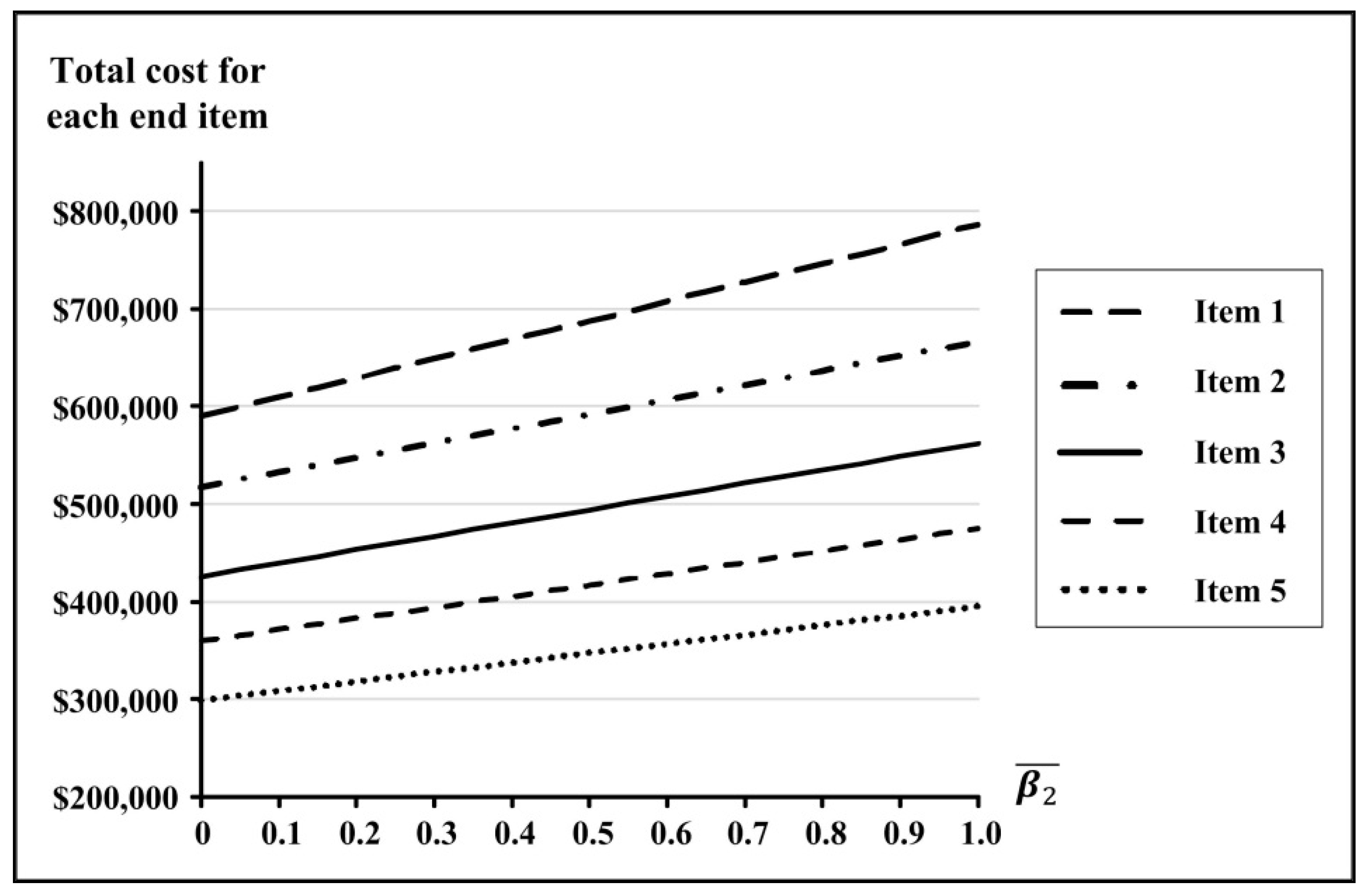
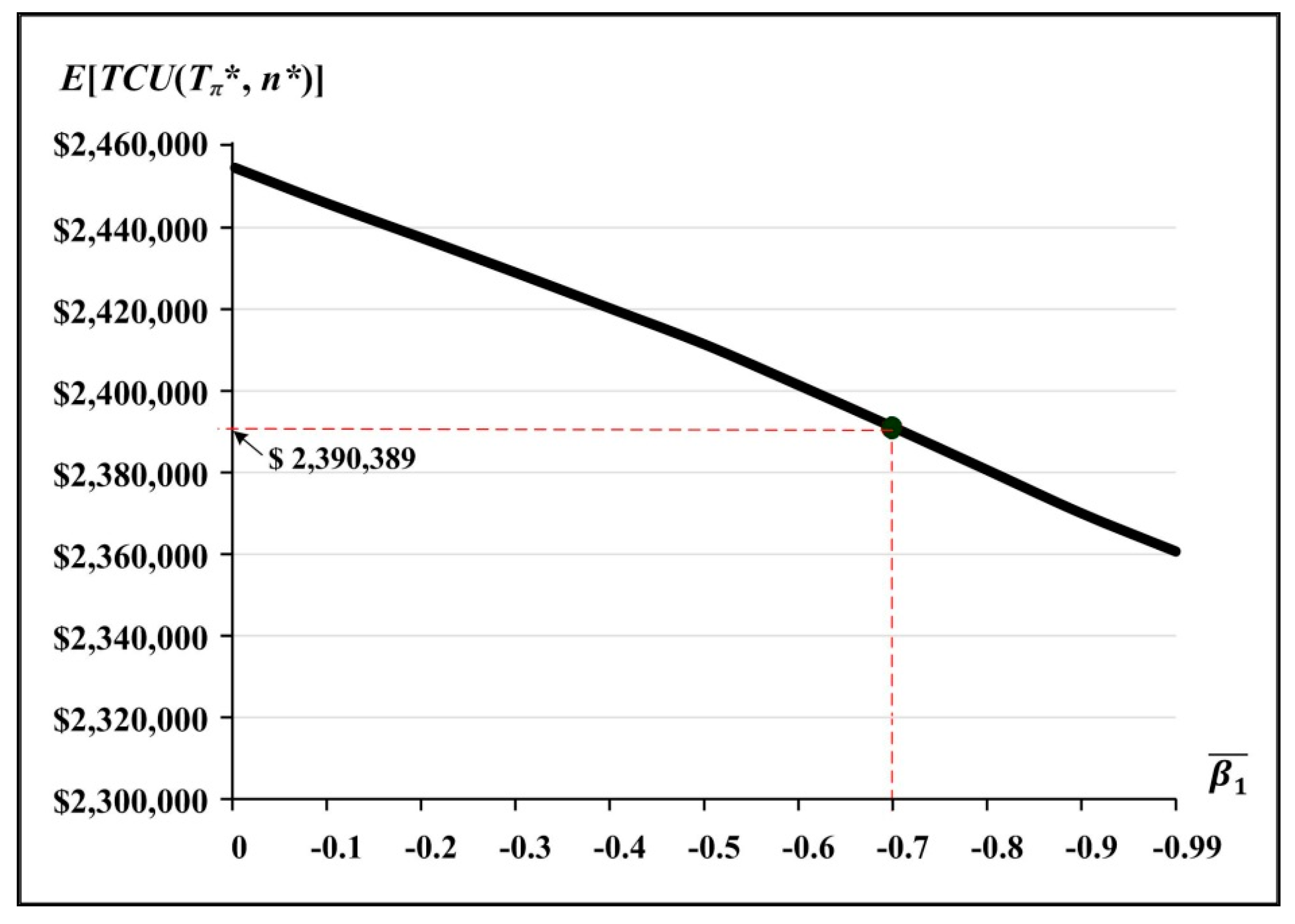
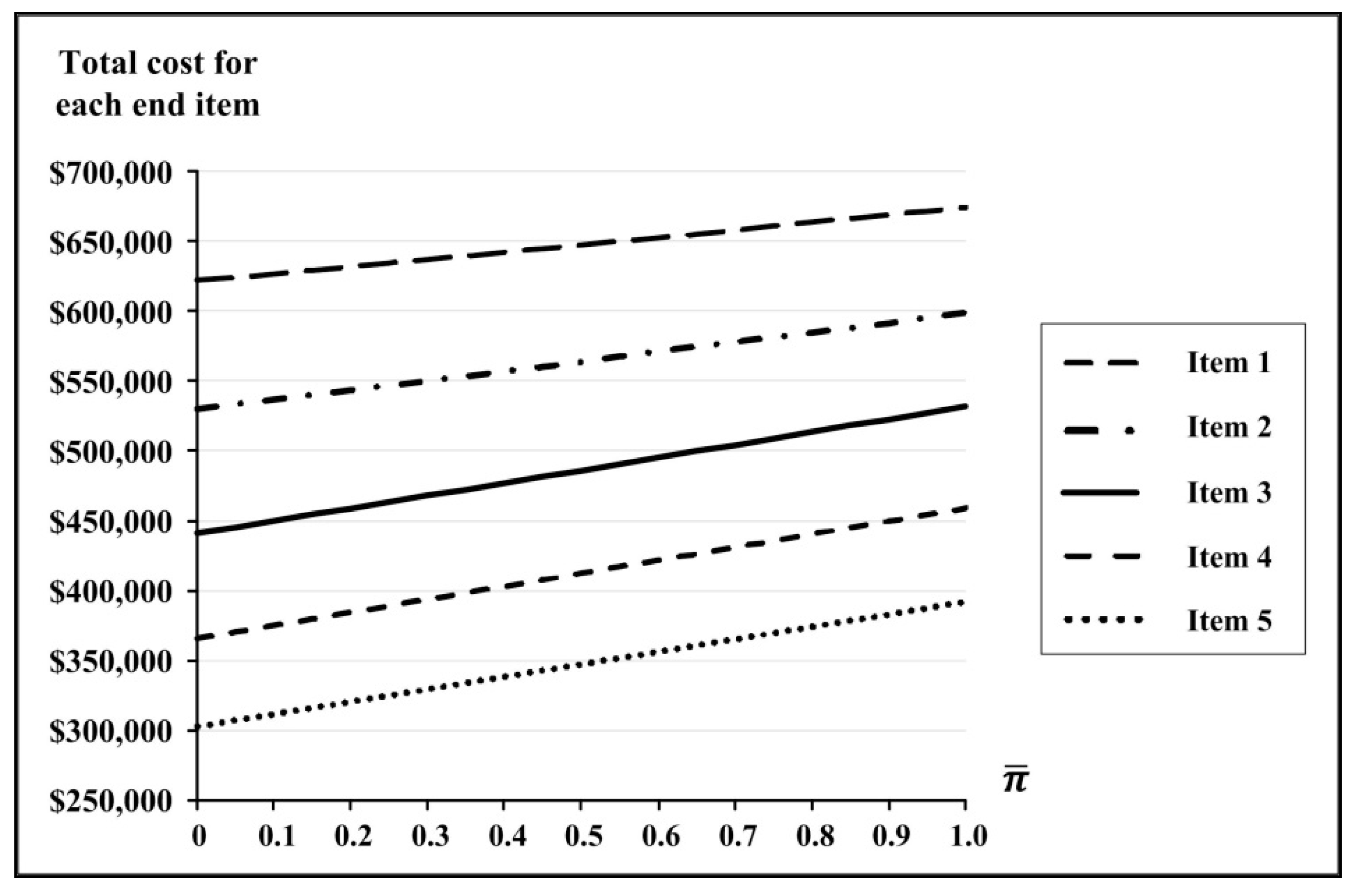
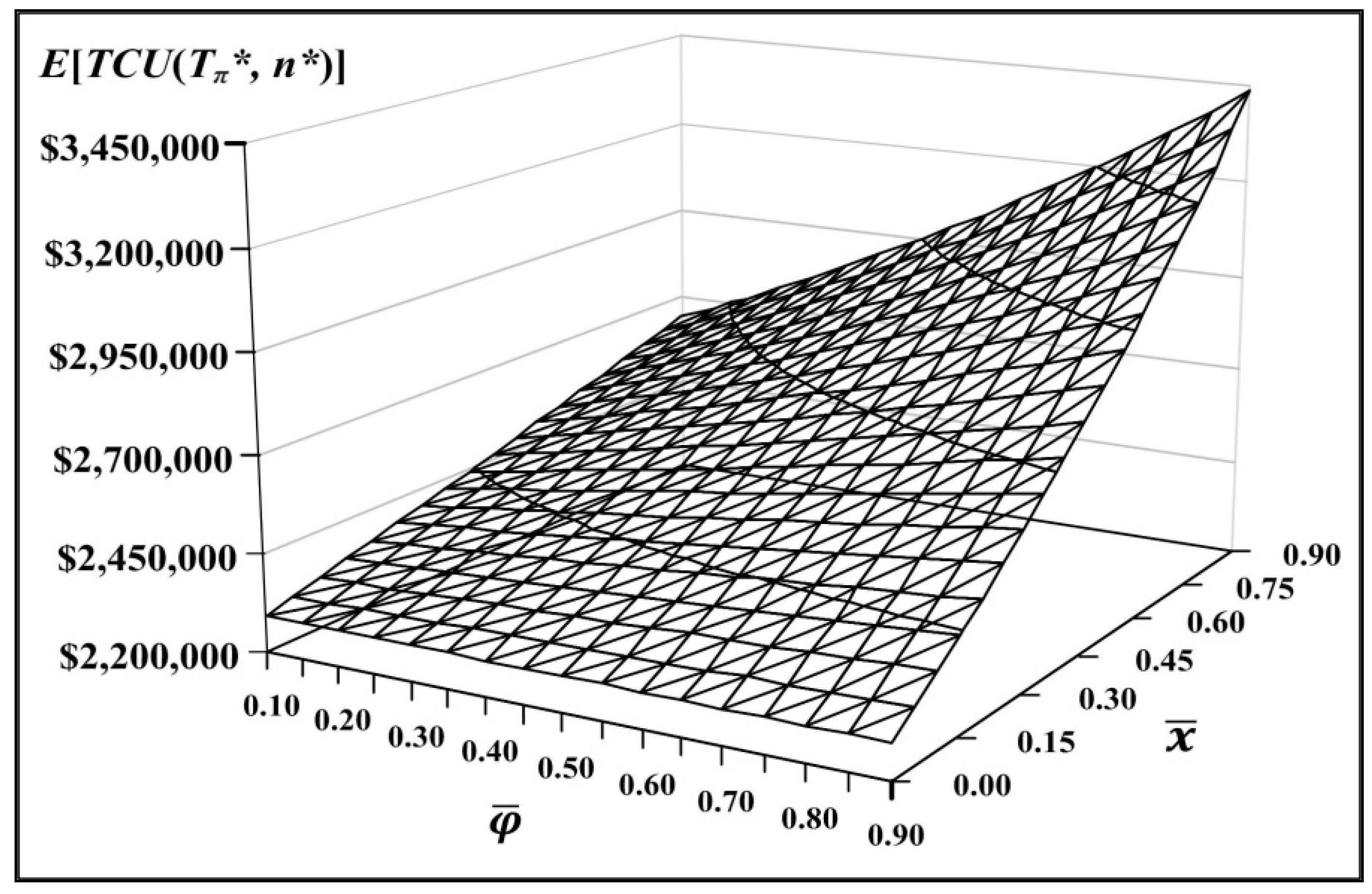
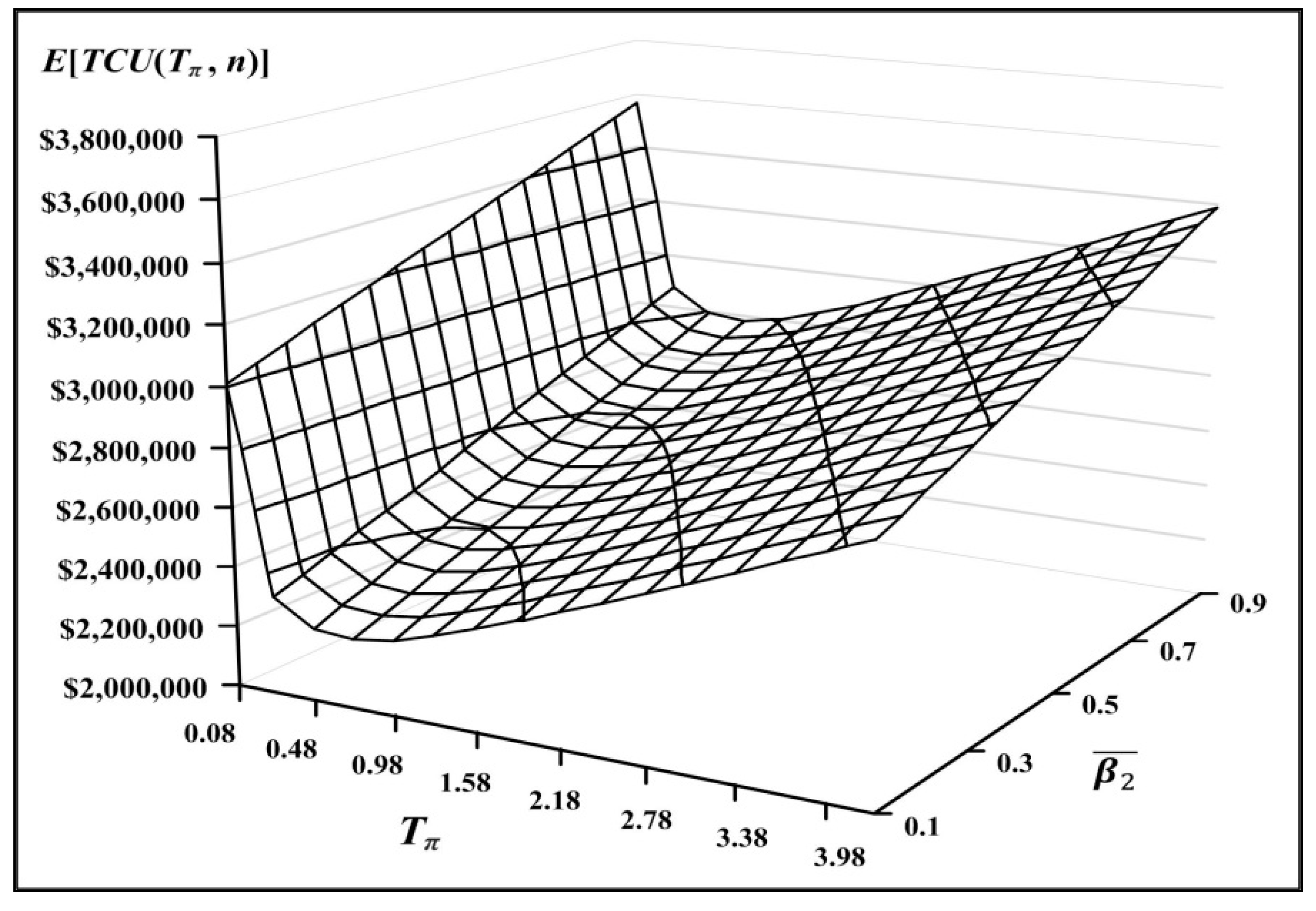
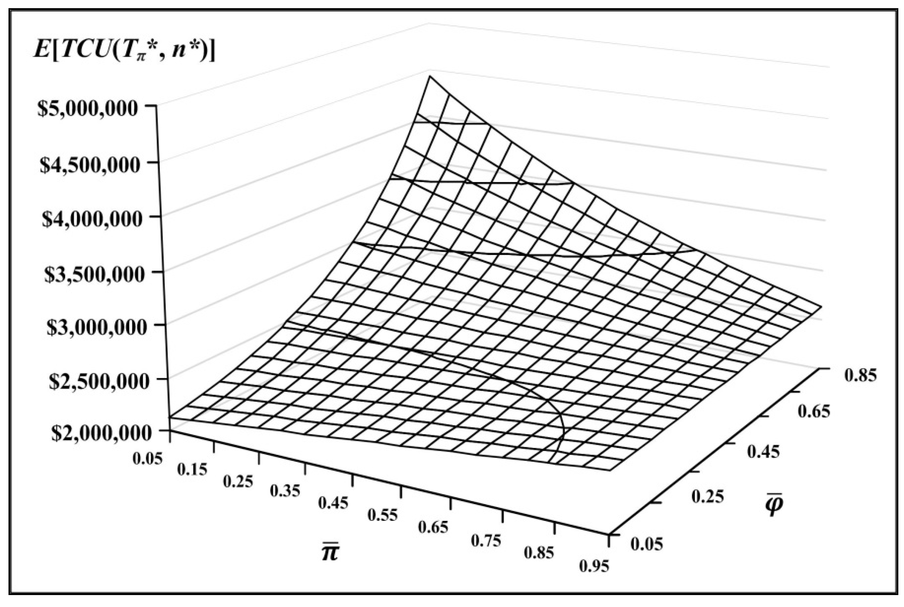
3.2. Joint Impacts from Combined System Factors
4. Conclusions
Author Contributions
Funding
Acknowledgments
Conflicts of Interest
Appendix A
Appendix B
Appendix C
Appendix D

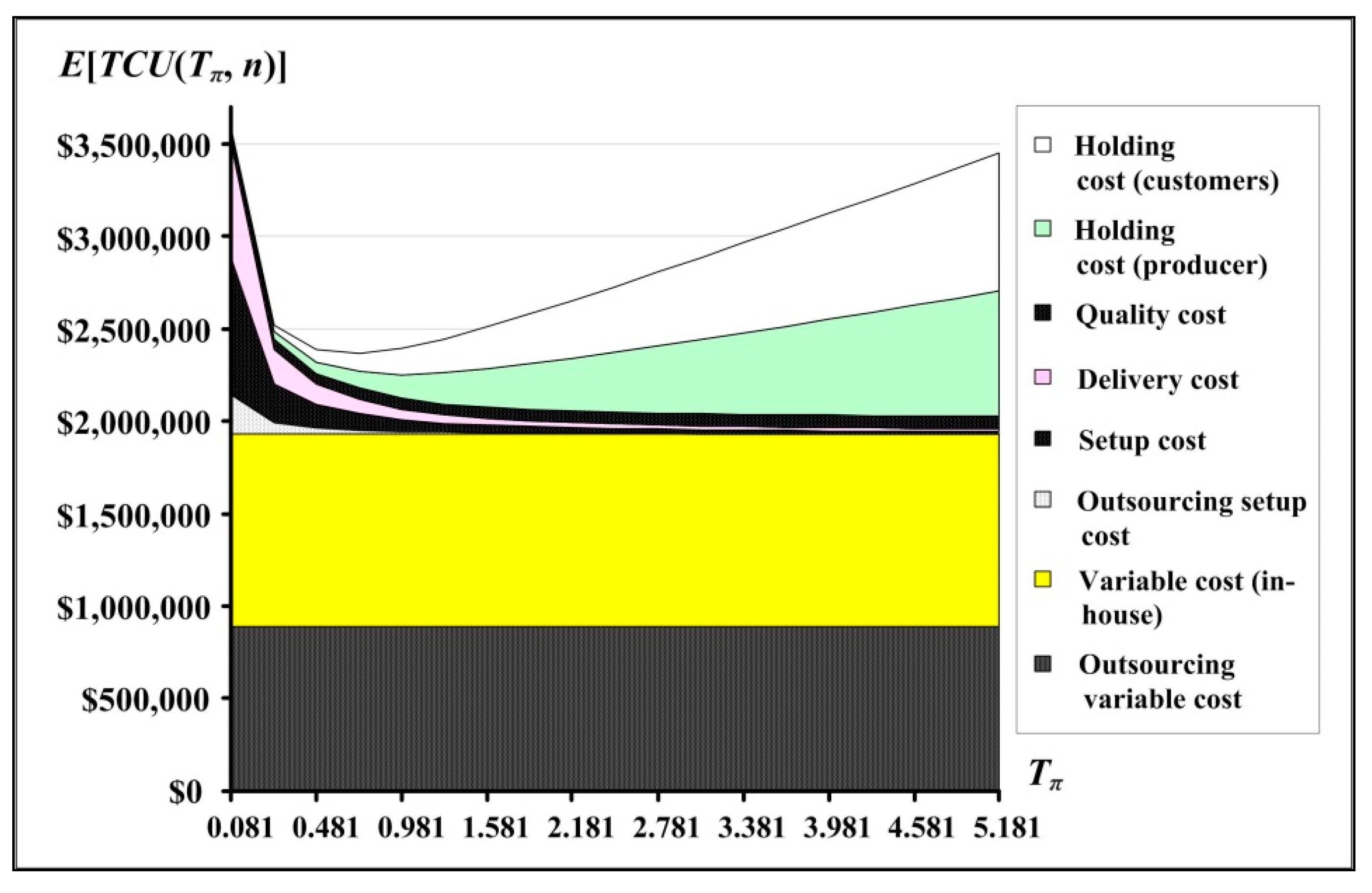
| n* | Tπ* | Annual System Cost E[TCU(Tπ*, n*)] (1) | Outsourcing Relating Cost (2) | % (2)/(1) | Quality Guarantee Cost (3) | % (3)/(1) | Delivery Cost (4) | % (4)/(1) | Customer Holding Cost (5) | % (5)/(1) | Other In-House Cost (6) | % (6)/(1) | |
|---|---|---|---|---|---|---|---|---|---|---|---|---|---|
| 0.00 | 3 | 0.5638 | $2,239,231 | $0 | 0% | $140,680 | 6.28% | $71,818 | 3.20% | $123,738 | 5.52% | $2,028,712 | 90.52% |
| 0.05 | 3 | 0.5684 | $2,286,723 | $144,275 | 6.31% | $130,833 | 5.72% | $71,272 | 3.12% | $123,358 | 5.39% | $1,816,985 | 79.46% |
| 0.10 | 3 | 0.5730 | $2,301,276 | $257,184 | 11.18% | $121,294 | 5.27% | $70,745 | 3.07% | $122,941 | 5.34% | $1,729,111 | 75.14% |
| 0.15 | 3 | 0.5775 | $2,315,912 | $369,772 | 15.97% | $112,062 | 4.84% | $70,237 | 3.03% | $122,486 | 5.29% | $1,641,354 | 70.87% |
| 0.20 | 3 | 0.5819 | $2,330,633 | $482,042 | 20.68% | $103,134 | 4.43% | $69,749 | 2.99% | $121,992 | 5.23% | $1,553,716 | 66.66% |
| 0.25 | 3 | 0.5861 | $2,345,440 | $593,995 | 25.33% | $94,508 | 4.03% | $69,280 | 2.95% | $121,458 | 5.18% | $1,466,199 | 62.51% |
| 0.30 | 3 | 0.5903 | $2,360,334 | $705,634 | 29.90% | $86,182 | 3.65% | $68,831 | 2.92% | $120,884 | 5.12% | $1,378,803 | 58.42% |
| 0.35 | 3 | 0.5943 | $2,375,317 | $816,961 | 34.39% | $78,154 | 3.29% | $68,402 | 2.88% | $120,268 | 5.06% | $1,291,532 | 54.37% |
| 0.40 | 3 | 0.5982 | $2,390,389 | $927,977 | 38.82% | $70,423 | 2.95% | $67,992 | 2.84% | $119,611 | 5.00% | $1,204,385 | 50.38% |
| 0.45 | 3 | 0.6019 | $2,405,551 | $1,038,685 | 43.18% | $62,985 | 2.62% | $67,603 | 2.81% | $118,912 | 4.94% | $1,117,365 | 46.45% |
| 0.50 | 3 | 0.6055 | $2,420,805 | $1,149,087 | 47.47% | $55,840 | 2.31% | $67,235 | 2.78% | $118,170 | 4.88% | $1,030,473 | 42.57% |
| 0.55 | 3 | 0.6089 | $2,436,150 | $1,259,185 | 51.69% | $48,984 | 2.01% | $66,886 | 2.75% | $117,386 | 4.82% | $943,708 | 38.74% |
| 0.60 | 3 | 0.6122 | $2,451,588 | $1,368,982 | 55.84% | $42,416 | 1.73% | $66,558 | 2.71% | $116,558 | 4.75% | $857,074 | 34.96% |
| 0.65 | 3 | 0.6152 | $2,467,120 | $1,478,478 | 59.93% | $36,135 | 1.46% | $66,251 | 2.69% | $115,688 | 4.69% | $770,569 | 31.23% |
| 0.70 | 3 | 0.6182 | $2,482,746 | $1,587,676 | 63.95% | $30,137 | 1.21% | $65,964 | 2.66% | $114,775 | 4.62% | $684,194 | 27.56% |
| 0.75 | 3 | 0.6209 | $2,498,466 | $1,696,577 | 67.90% | $24,421 | 0.98% | $65,698 | 2.63% | $113,819 | 4.56% | $597,950 | 23.93% |
| 0.80 | 3 | 0.6234 | $2,514,280 | $1,805,185 | 71.80% | $18,985 | 0.76% | $65,453 | 2.60% | $112,820 | 4.49% | $511,837 | 20.36% |
| 0.85 | 3 | 0.6257 | $2,530,190 | $1,913,500 | 75.63% | $13,827 | 0.55% | $65,228 | 2.58% | $111,780 | 4.42% | $425,854 | 16.83% |
| 0.90 | 3 | 0.6279 | $2,546,195 | $2,021,525 | 79.39% | $8,945 | 0.35% | $65,024 | 2.55% | $110,698 | 4.35% | $340,002 | 13.35% |
| 0.95 | 3 | 0.6298 | $2,562,294 | $2,129,261 | 83.10% | $4,336 | 0.17% | $64,841 | 2.53% | $109,576 | 4.28% | $254,279 | 9.92% |
| 1.00 | 3 | 0.6315 | $2,483,483 | $2,236,710 | 90.06% | $0 | 0% | $64,679 | 2.60% | $108,415 | 4.37% | $73,680 | 2.97% |
| n* | Tπ* | Sum of Manufacture –ing Uptime (in Year) | Sum of Rework Time (in Year) | Machine Idle Time Per Cycle (in Year) | Utilization (Uptime) (A) | Utilization (Rework Time) (B) | Total Utilization (A) + (B) | |
|---|---|---|---|---|---|---|---|---|
| 0.00 | 3 | 0.5638 | 0.1638 | 0.2070 | 0.1930 | 0.291 | 0.367 | 0.658 |
| 0.05 | 3 | 0.5684 | 0.1567 | 0.1980 | 0.2137 | 0.276 | 0.348 | 0.624 |
| 0.10 | 3 | 0.5730 | 0.1494 | 0.1887 | 0.2349 | 0.261 | 0.329 | 0.590 |
| 0.15 | 3 | 0.5775 | 0.1420 | 0.1793 | 0.2562 | 0.246 | 0.310 | 0.556 |
| 0.20 | 3 | 0.5819 | 0.1345 | 0.1698 | 0.2776 | 0.231 | 0.292 | 0.523 |
| 0.25 | 3 | 0.5861 | 0.1269 | 0.1600 | 0.2992 | 0.217 | 0.273 | 0.490 |
| 0.30 | 3 | 0.5903 | 0.1191 | 0.1502 | 0.3210 | 0.202 | 0.254 | 0.456 |
| 0.35 | 3 | 0.5943 | 0.1112 | 0.1401 | 0.3430 | 0.187 | 0.236 | 0.423 |
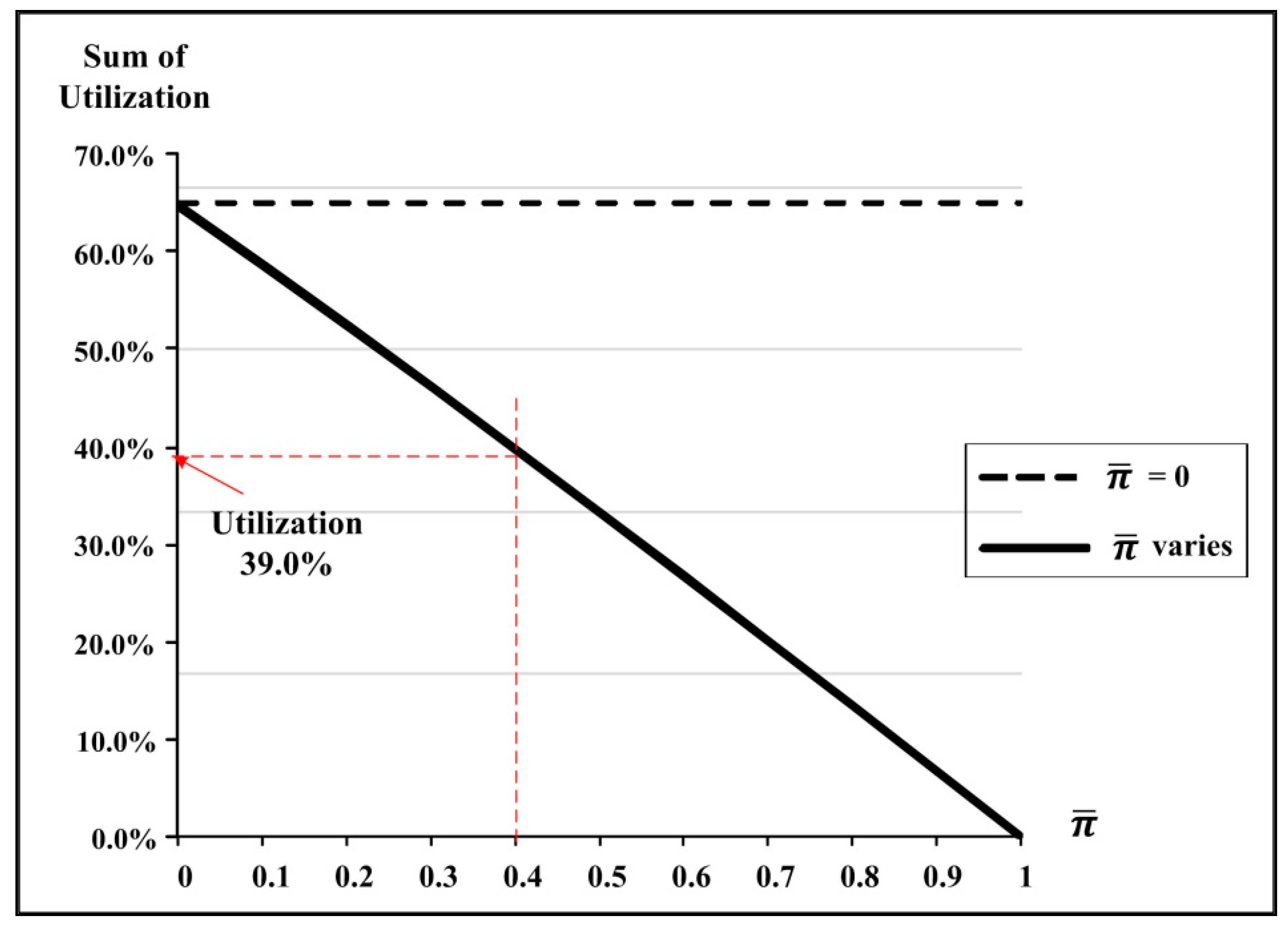
| 0.40 | 3 | 0.5982 | 0.1032 | 0.1300 | 0.3650 | 0.173 | 0.217 | 0.390 |
| 0.45 | 3 | 0.6019 | 0.0950 | 0.1197 | 0.3872 | 0.158 | 0.199 | 0.357 |
| 0.50 | 3 | 0.6055 | 0.0868 | 0.1093 | 0.4094 | 0.143 | 0.181 | 0.324 |
| 0.55 | 3 | 0.6089 | 0.0784 | 0.0987 | 0.4318 | 0.129 | 0.162 | 0.291 |
| 0.60 | 3 | 0.6122 | 0.0700 | 0.0881 | 0.4541 | 0.114 | 0.144 | 0.258 |
| 0.65 | 3 | 0.6152 | 0.0615 | 0.0773 | 0.4764 | 0.100 | 0.126 | 0.226 |
| 0.70 | 3 | 0.6182 | 0.0529 | 0.0665 | 0.4988 | 0.086 | 0.108 | 0.193 |
| 0.75 | 3 | 0.6209 | 0.0442 | 0.0556 | 0.5211 | 0.071 | 0.090 | 0.161 |
| 0.80 | 3 | 0.6234 | 0.0355 | 0.0446 | 0.5433 | 0.057 | 0.072 | 0.128 |
| 0.85 | 3 | 0.6257 | 0.0267 | 0.0335 | 0.5655 | 0.043 | 0.054 | 0.096 |
| 0.90 | 3 | 0.6279 | 0.0178 | 0.0224 | 0.5877 | 0.028 | 0.036 | 0.064 |
| 0.95 | 3 | 0.6298 | 0.0089 | 0.0112 | 0.6097 | 0.014 | 0.018 | 0.032 |
| 1.00 | 3 | 0.6315 | 0.0000 | 0.0000 | 0.6315 | 0.000 | 0.000 | 0.000 |
References
- Lee, S.M.; Clayton, E.R.; Taylor, B.W., III. A goal programming approach to multi-period production line scheduling. Comput. Oper. Res. 1978, 5, 205–211. [Google Scholar] [CrossRef]
- Rosenblatt, M.J. Fixed cycle, basic cycle and EOQ approaches to the multi-item single supplier inventory system. Int. J. Prod. Res. 1985, 23, 1131–1139. [Google Scholar] [CrossRef]
- Kohli, R.; Park, H. Coordinating buyer-seller transactions across multiple products. Manag. Sci. 1994, 40, 45–50. [Google Scholar] [CrossRef]
- Sambasivan, M.; Schmidt, C.P. A heuristic procedure for solving multi-plant, multi-item, multi-period capacitated lot-sizing problems. Asia-Pac. J. Oper. Res. 2002, 19, 87–105. [Google Scholar]
- Taleizadeh, A.A.; Widyadana, G.A.; Wee, H.M.; Biabani, J. Multi products single machine economic production quantity model with multiple batch size. Int. J. Ind. Eng. Comput. 2011, 2, 213–224. [Google Scholar] [CrossRef]
- Vujosevic, M.; Makajic-Nikolic, D.; Pavlovic, P. A new approach to determination of the most critical multi-state components in multi-state systems. J. Appl. Eng. Sci. 2017, 15, 401–405. [Google Scholar] [CrossRef] [Green Version]
- Chiu, Y.-S.P.; Lin, H.-D.; Wu, M.-F.; Chiu, S.W. Alternative fabrication scheme to study effects of rework of nonconforming products and delayed differentiation on a multiproduct supply- chain system. Int. J. Ind. Eng. Comput. 2018, 9, 235–248. [Google Scholar] [CrossRef]
- Chiu, S.W.; Kuo, J.-S.; Chiu, Y.-S.P.; Chang, H.-H. Production and distribution decisions for a multi-product system with component commonality, postponement strategy and quality assurance using a two-machine scheme. Jordan J. Mech. Ind. Eng. 2019, 13, 105–115. [Google Scholar]
- Bhuniya, S.; Sarkar, B.; Pareek, S. Multi-product production system with the reduced failure rate and the optimum energy consumption under variable demand. Mathematics 2019, 7, 465. [Google Scholar] [CrossRef] [Green Version]
- Chiu, S.W.; Huang, Y.-J.; Chiu, Y.-S.P.; Chiu, T. Satisfying multiproduct demand with a FPR-based inventory system featuring expedited rate and scraps. Int. J. Ind. Eng. Comput. 2019, 10, 443–452. [Google Scholar] [CrossRef]
- Prencipe, A. Technological competencies and product’s evolutionary dynamics a case study from the aero-engine industry. Res. Policy 1997, 25, 1261–1276. [Google Scholar] [CrossRef]
- Kouvelis, P.; Milner, J.M. Supply chain capacity and outsourcing decisions: The dynamic interplay of demand and supply uncertainty. IIE Trans. 2002, 34, 717–728. [Google Scholar] [CrossRef]
- Wee, H.-M.; Peng, S.-Y.; Wee, P.K.P. Modelling of outsourcing decisions in global supply chains—An empirical study on supplier management performance with different outsourcing strategies. Int. J. Prod. Res. 2010, 48, 2081–2094. [Google Scholar] [CrossRef]
- Chraibi, S.; Sauvage, T.; Sbihi, A.; Cragg, T. An exploratory model for outsourcing- purchasing activities based on a comparative study. Supply Chain Forum: Int. J. 2017, 18, 138–149. [Google Scholar] [CrossRef]
- Arya, A.; Mittendorf, B.; Sappington, D.E.M. The make-or-buy decision in the presence of a rival: Strategic outsourcing to a common supplier. Manag. Sci. 2008, 54, 1747–1758. [Google Scholar] [CrossRef] [Green Version]
- Chiu, Y.-S.P.; Liu, C.-J.; Hwang, M.-H. Optimal batch size considering partial outsourcing plan and rework. Jordan J. Mech. Ind. Eng. 2017, 11, 195–200. [Google Scholar]
- Mohammadi, M. The tradeoff between outsourcing and using more factories in a distributed flow shop system. Econ. Comput. Econ. Cybern. Stud. Res. 2017, 51, 279–295. [Google Scholar]
- Chiu, S.W.; Liu, C.-J.; Li, Y.-Y.; Chou, C.-L. Manufacturing lot size and product distribution problem with rework, outsourcing and discontinuous inventory distribution policy. Int. J. Eng. Model. 2017, 30, 49–61. [Google Scholar]
- Chiu, Y.-S.P.; Chiu, V.; Lin, H.-D.; Chang, H.-H. Meeting multiproduct demand with a hybrid inventory replenishment system featuring quality reassurance. Oper. Res. Persp. 2019, 6, 100112. [Google Scholar] [CrossRef]
- Dohi, T.; Kaio, N.; Osaki, S. Minimal repair policies for an economic manufacturing process. J. Qual. Maint. Eng. 1998, 4, 248–262. [Google Scholar] [CrossRef]
- Inderfurth, K.; Janiak, A.; Kovalyov, M.Y.; Werner, F. Batching work and rework processes with limited deterioration of reworkables. Comput. Oper. Res. 2006, 33, 1595–1605. [Google Scholar] [CrossRef] [Green Version]
- Makarova, I.; Shubenkova, K.; Mavrin, V.; Boyko, A. Ways to increase sustainability of the transportation system. J. Appl. Eng. Sci. 2017, 15, 89–98. [Google Scholar] [CrossRef] [Green Version]
- Rao, A.S.; Singh, A.K. Failure analysis of stainless steel lanyard wire rope. J. Appl. Res. Technol. 2018, 16, 35–40. [Google Scholar] [CrossRef] [Green Version]
- Khanna, A.; Kishore, A.; Sarkar, B.; Jaggi, C.K. Supply chain with customer-based two-level credit policies under an imperfect quality environment. Mathematics 2018, 6, 299. [Google Scholar] [CrossRef] [Green Version]
- Ben Fathallah, B.; Saidi, R.; Dakhli, C.; Belhadi, S.; Yallese, M.A. Mathematical modelling and optimization of surface quality and productivity in turning process of aisi 12l14 free-cutting steel. Int. J. Ind. Eng. Comput. 2019, 10, 557–576. [Google Scholar] [CrossRef]
- Banerjee, A.; Banerjee, S. Coordinated order-less inventory replenishment for a vendor and multiple buyers. Int. J. Technol. Manag. 1992, 7, 328–336. [Google Scholar]
- Viswanathan, S.; Piplani, R. Coordinating supply chain inventories through common replenishment epochs. Eur. J. Oper. Res. 2001, 129, 277–286. [Google Scholar] [CrossRef]
- Sancak, E.; Salmann, F.S. Multi-item dynamic lot-sizing with delayed transportation policy. Int. J. Prod. Econ. 2011, 131, 595–603. [Google Scholar] [CrossRef]
- Dey, B.K.; Sarkar, B.; Pareek, S. A two-echelon supply chain management with setup time and cost reduction, quality improvement and variable production rate. Mathematics 2019, 7, 328. [Google Scholar] [CrossRef] [Green Version]
- Chiu, Y.-S.P.; Jhan, J.-H.; Chiu, V.; Chiu, S.W. Fabrication cycle time and shipment decision for a multiproduct intra-supply chain system with external source and scrap. Int. J. Math. Eng. Manag. Sci. 2020, 5, 614–630. [Google Scholar] [CrossRef]
- Rossit, D.G.; Gonzalez, M.E.; Tohmé, F.; Frutos, M. Upstream logistic transport planning in the oil-industry: A case study. Int. J. Ind. Eng. Comput. 2020, 11, 221–234. [Google Scholar] [CrossRef]
- Imran, M.; Habib, M.S.; Hussain, A.; Ahmed, N.; Al-Ahmari, A.M. Inventory routing problem in supply chain of perishable products under cost uncertainty. Mathematics 2020, 8, 382. [Google Scholar] [CrossRef] [Green Version]
- Chiu, Y.-S.P.; Chiu, S.W.; Li, C.-Y.; Ting, C.-K. Incorporating multi-delivery policy and quality assurance into economic production lot size problem. J. Sci. Ind. Res. 2009, 68, 505–512. [Google Scholar]
- Rardin, R.L. Optimization in Operations Research; Prentice-Hall: Upper Saddle River, NJ, USA, 1998. [Google Scholar]
- Nahmias, S. Production & Operations Analysis; McGraw-Hill Co. Inc.: New York, NY, USA, 2009. [Google Scholar]


| Tπ | rotation cycle time; |
| Qi | batch size for product i, |
| Ki | in-house setup cost for product i, |
| Ci | unit in-house manufacturing cost for product i, |
| hi | unit holding cost of product i, |
| h1i | unit holding cost for reworked product i, |
| h2i | unit holding cost in the retailer side, |
| CSi | unit disposal cost, |
| t1iπ | uptime for product i, |
| t2iπ | rework time, |
| t3iπ | delivery time, |
| tniπ | fixed interval of time between deliveries, |
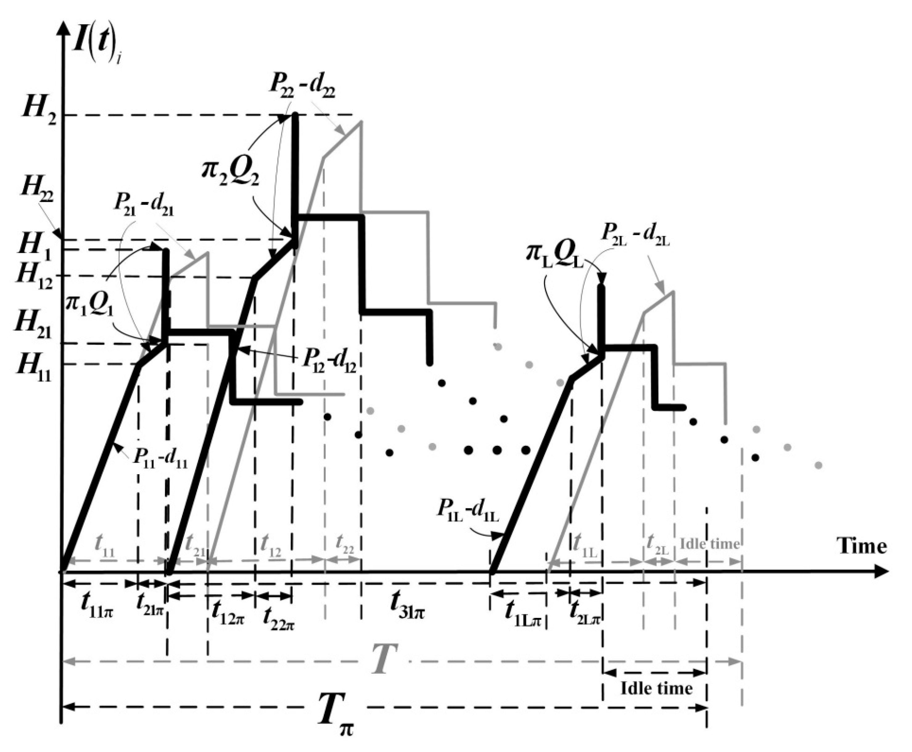
| H1i | inventory level when the uptime ends, |
| H2i | inventory level when the rework time ends, |
| Hi | maximum inventory level in the beginning of delivery time (after receipt of outsourced items), |
| N | number of shipments per cycle − another decision variable, |
| K1i | fixed delivery cost for product i, |
| CTi | unit delivery cost, |
| I(t)i | stock level of finished items at time t, |
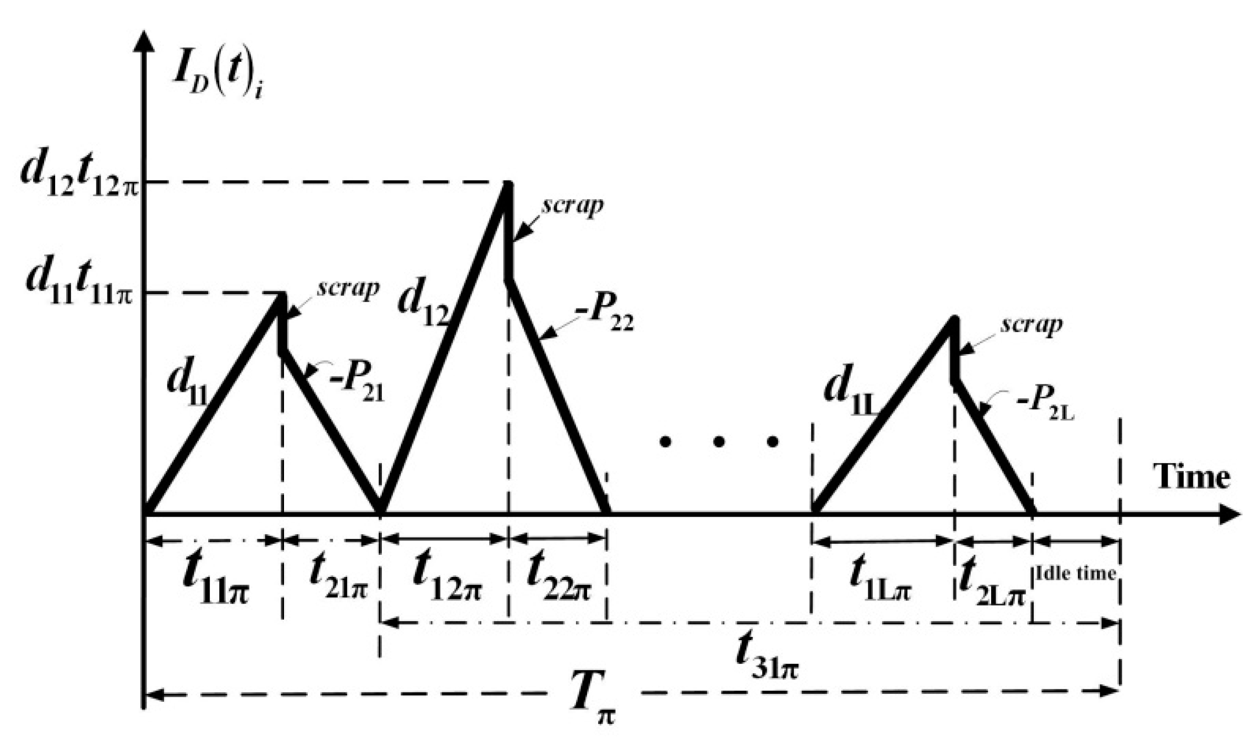
| ID(t)i | inventory level of defective items, |
| IS(t)i | inventory level of scrap, |
| Ic(t)i | stock level of product i in the retailer’s side at time t, |
| t1i | uptime for the product i in the proposed system without outsourcing plan, |
| t2i | rework time in a system without outsourcing, |
| t3i | delivery time in a system without outsourcing, |
| T | rotation cycle time a system without outsourcing, |
| TC(Tπ, n) | total cost per cycle, |
| E[TCU(Tπ, n)] | the long-run average system cost per unit time, |
| End Item No. | Ci | β2i | Cπi | Ki | β1i | Kπi | λi | πi | P1i | P2i | |
| 1 | 80 | 0.40 | 112.0 | 10,000 | −0.60 | 4000 | 3000 | 0.4 | 58,000 | 2900 | |
| 2 | 90 | 0.35 | 121.5 | 11,000 | −0.65 | 3850 | 3200 | 0.4 | 59,000 | 2950 | |
| 3 | 100 | 0.30 | 130.0 | 12,000 | −0.70 | 3600 | 3400 | 0.4 | 60,000 | 3000 | |
| 4 | 110 | 0.25 | 137.5 | 13,000 | −0.75 | 3250 | 3600 | 0.4 | 61,000 | 3050 | |
| 5 | 120 | 0.20 | 144.0 | 14,000 | −0.80 | 2800 | 3800 | 0.4 | 62,000 | 3100 | |
| End Item No. | xi | CRi | CSi | K1i | CTi | hi | h1i | h2i | θ1i | θ2i | φi |
| 1 | 5% | 50 | 20 | 2300 | 0.1 | 10 | 30 | 50 | 0.05 | 0.05 | 0.0975 |
| 2 | 10% | 55 | 25 | 2400 | 0.2 | 15 | 35 | 55 | 0.10 | 0.10 | 0.1900 |
| 3 | 15% | 60 | 30 | 2500 | 0.3 | 20 | 40 | 60 | 0.15 | 0.15 | 0.2775 |
| 4 | 20% | 65 | 35 | 2600 | 0.4 | 25 | 45 | 65 | 0.20 | 0.20 | 0.3600 |
| 5 | 25% | 70 | 40 | 2700 | 0.5 | 30 | 50 | 70 | 0.25 | 0.25 | 0.4375 |
Publisher’s Note: MDPI stays neutral with regard to jurisdictional claims in published maps and institutional affiliations. |
© 2020 by the authors. Licensee MDPI, Basel, Switzerland. This article is an open access article distributed under the terms and conditions of the Creative Commons Attribution (CC BY) license (http://creativecommons.org/licenses/by/4.0/).
Share and Cite
Chiu, Y.-S.P.; Chiu, V.; Yeh, T.-M.; Wu, H.-Y. Incorporating Outsourcing Strategy and Quality Assurance into a Multiproduct Manufacturer–Retailer Coordination Replenishing Decision. Mathematics 2020, 8, 2212. https://doi.org/10.3390/math8122212
Chiu Y-SP, Chiu V, Yeh T-M, Wu H-Y. Incorporating Outsourcing Strategy and Quality Assurance into a Multiproduct Manufacturer–Retailer Coordination Replenishing Decision. Mathematics. 2020; 8(12):2212. https://doi.org/10.3390/math8122212
Chicago/Turabian StyleChiu, Yuan-Shyi Peter, Victoria Chiu, Tsu-Ming Yeh, and Hua-Yao Wu. 2020. "Incorporating Outsourcing Strategy and Quality Assurance into a Multiproduct Manufacturer–Retailer Coordination Replenishing Decision" Mathematics 8, no. 12: 2212. https://doi.org/10.3390/math8122212