Article

Scheduling Optimization in Flowline Manufacturing Cell Considering Intercell Movement with Harmony Search Approach

School of Mechanical Engineering and Automation, Beihang University, Beijing 100191, China
*
Author to whom correspondence should be addressed.
Mathematics 2020, 8(12), 2225; https://doi.org/10.3390/math8122225
Submission received: 16 November 2020 / Revised: 7 December 2020 / Accepted: 10 December 2020 / Published: 14 December 2020

Abstract

:
Based on the non-permutation property of intercell scheduling in flowline manufacturing cells, a hybrid harmony search algorithm is proposed to solve the problem with the makespan criterion. On the basis of the basic harmony search algorithm, the three key elements of memory consideration, pitch adjustment and random selection are discretized and improved to adapt to the operation-based encoding. To compare the performance, different scale cases are generated in both the overall solution and the two-stage solution with the proposed algorithm, the hybrid particle swarm optimization algorithm and the hybrid genetic algorithm. The relative deviation is taken as the performance index. The compared results show that a better solution can be obtained with the proposed algorithm in both the overall solution and the two-stage solution, verifying the superior performance of the proposed algorithm.

1. Introduction

Based on the important idea of management and manufacturing in group technology (GT), cell manufacturing (CM) mainly carries out cell production by grouping similar parts (tasks) and process equipment (machines). In each production cell, several part families are processed on the machines of the cell, and each manufacturing cell works together to form a cell manufacturing system (CMS) [1]. Each cell produces a series of specific products according to the part family. These part families are generally formed according to the processes, machines, tools, etc. In addition to reducing the cost of setup time, the main advantage of CMS is to simplify material flow. Moreover, the professional skills of operators are improved, repetitive work is reduced and production time is shortened, and reports show that material flow and production costs can be reduced. Flowline manufacturing cell scheduling is the application and scheduling of flow shop production mode in the cell manufacturing environment, that is, the task family of each production cell and the tasks within the family are processed through all machines of the cell according to a certain production technology, and a reasonable processing sequence is arranged to make one or some performance achieve the optimal. The common performance indicators include the minimum maximum completion time (makespan) [2], total tardiness [3] and mean flow time [4].
The realization of CMS is divided into three stages: cell formation, cell layout and cell scheduling. As the design stages of CMS, cell formation is to group jobs and machines, and cell layout solves the location layout problem of cells and production machines. As the production planning stage of CMS, cell scheduling plays an important role, mainly deciding the scheduling problem of jobs intra- and intercells.
An important goal of cell manufacturing is to form independent cells. Unfortunately, in many real manufacturing systems, it is impossible for completely autonomous manufacturing cells to exist [5]. On the contrary, it is inevitable to process jobs across cells. The statistics of 32 companies in the United States show that 25.8% to 34.3% of the operations need to be processed in foreign cells [6]. More than 50% of all processing routes need intercell transfers in the Chinese manufacturing industry [7]. In these CMS, parts that need to be processed in multiple cells are known as exceptional elements, while the machines that are used by the parts are called bottleneck machines. Besides the fact that exceptional elements may be a result of the cell formation process, there are also some other factors, such as painting and thermal processing, that have to be conducted by a single machine for parts from multiple cells, due to the low utilization rate of equipment, machine immobility, toxicity or high investment of processing process; thus, a separate equipment is needed for processing [8]. Moreover, exceptional elements are not only produced in the design and application of CMS, but also exist in the whole process of CMS running. Changes in product design, function and production quality can gradually lead to specific parts being processed in machines located in different cells [9]. At the operation level, the change of workload between cells, such as transferring operations to machines with low utilization of foreign processing cells, can significantly improve workshop performance [10]. Similarly, the transportation of intercells can reduce severe machine failures and prevent production defects [11].
Compared with the existing literature, the main contributions of this paper include three aspects:
  • The intercell scheduling problem is solved with non-permutation flow shop cells, aiming to minimize makespan.
  • A hybrid harmony search algorithm (HHS) is proposed. The three key elements of memory consideration, pitch adjustment and random selection are improved to adapt to the operation-based encoding. Moreover, first in first out (FIFO) rules are integrated into the two-stage solution to deal with the intercell scheduling problem.
  • Compare the performance of the two existing solutions of intercell scheduling, the global solution and the two-stage solution.
The remainder part of this paper is organized as follows: Section 2 reviews the flowline manufacturing cell scheduling and harmony search algorithms. The problem is described in Section 3. Section 4 introduces the proposed improved harmony search algorithm. The analysis of the experimental results are reported in Section 5. Finally, Section 6 provides conclusions.

2. Literature Review

A flowline manufacturing cell is a common production layout in the manufacturing industry. The scheduling of flowline manufacturing cells has been studied by many scholars internationally. Neufeld et al. [12] summarized the flow shop group scheduling in detail. Baker [13] studied the two-machine flow shop, considering the time lags or sequence-independent setup time. Wemmerlov and Vakharia [14] developed two heuristic programs to solve the part family scheduling of flowline manufacturing cells with three or more machines. Skorin-Kapov and Vakharia [15] developed six tabu search heuristics. And Sridhar and Rajendran [16] developed a genetic algorithm to minimize makespan for the part scheduling in the flowline manufacturing cell. Logendran et al. [17] and Schaller [18] studied the performance comparison of some hybrid heuristic algorithms for scheduling in the flowline manufacturing cell. Reddy and Narendran [19] proposed a heuristic algorithm for scheduling with sequence-dependent setup time to improve the machine utilization in the flowline manufacturing cell. Logendran et al. [20] developed an LN-PT method to minimize the makespan for group scheduling in flexible flow shop, considering single and multiple setup times on the machine. Logendran et al. [21] proposed a tabu search algorithm to solve the group scheduling problem in flexible flow shop considering sequence dependence. Gupta and Schaller [22] proposed a branch and bound algorithm, which can solve the medium scale problems of flowline manufacturing cells with sequence-independent setup time. Hendizadeh et al. [23] proposed a tabu search meta heuristic algorithm to minimize makespan. Venkataramanaian [24] developed a simulated annealing-based algorithm to solve three objectives (minimum weighted makespan, total flow time and idle time). Zandieh et al. [25] proposed three meta heuristics based on tabu search, simulated annealing and genetic algorithm, and applied them to group scheduling problem with a sequence-dependent setup time. Ying et al. [26] solved the permutation and non-permutation scheduling problems in flowline manufacturing cells considering sequence dependent family setup time. Salmasi et al. [27] proposed a mathematical programming model to minimize the total flow time to solve the group scheduling problem in flow shop.
Although there are a lot of articles on cell formation and cell scheduling, few studies consider the intercell scheduling problem. In theory, the bottleneck can be eliminated by configuring multiple bottleneck machines (which can be moved among cells), or the exceptional tasks (which need to be processed by other cells) can be outsourced. However, neither kind of measure, based on the consideration of manufacturing cost, budget and manufacturing cell space constraints, is realistic. Therefore, in a typical CMS environment, it is very difficult to form independent manufacturing cells. There will always be some bottleneck machines or exceptional tasks that will cause the existence of intercells, so intercell scheduling is inevitable. Yang and Liao [28] studied the group scheduling on two cells with intercell movement, and used branch and bound algorithm and heuristic algorithm to minimize the average flow time. However, this method is limited to two cells, and each part has only one operation. Therefore, Solimanpur et al. [29] proposed a two-stage heuristic algorithm SVS to solve the cell scheduling problem with intercell characteristics. Tavakkoli-Moghaddam et al. [30] considered the multi criteria cost function and the sequence dependent setup time, using the discrete search method to sort the cells and the jobs in the cell simultaneously. Mosbah and Dao [31] proposed an Extended Great Deluge (EGD) method to minimize makespan and a multi-criteria objective function. Solimanpur and Elmi [32] proposed a mixed integer linear programming model for the cell scheduling problem with the goal of minimizing makespan, which was solved by the tabu search algorithm. Neufeld [33] solved the intercell scheduling problem in flowline manufacturing cells, considering material flow and non-permutation scheduling. Li et al. [34] presented a pheromone-based approach (PBA), using multi-agent, aiming to solve the problem of scheduling with flexible processing routes, and exceptional parts, which need to visit machines located in multiple job shop cells.
Harmony search (HS) is a new intelligent optimization algorithm. By repeatedly adjusting the solution variables in the memory, the function value converges with the increase of iterations. The algorithm has the advantages of being a simple concept, having fewer adjustable parameters and being easy to implement. Compared with the basic genetic algorithm (GA), HS has two advantages: one advantage is to make full use of the existing harmony information in the harmony memory, though information on only two parents is used in GA; the other advantage is that HS considers each piece of individual information separately, but GA can only design the whole structure of one individual.
The simulated annealing algorithm is similar to the simulation of physical annealing, the genetic algorithm is similar to the simulation of biological evolution, and the particle swarm optimization algorithm is similar to the simulation of bird swarm, while the HS algorithm simulates the principle of music performance. The HS algorithm is a meta heuristic algorithm proposed by GEEM [35]. It is a population-based metaheuristic algorithm. It is inspired by the music creation process. The purpose of the HS algorithm is to let each music player find a better harmony state. Because of its simplicity and ease of application, HS has been successfully used to deal with a large number of optimization problems [36,37,38,39,40,41,42,43,44,45,46,47].
HS is also successfully used to solve the production scheduling problem. For the just in time (JIT) constrained single machine earliness/tardiness scheduling problem, Liu and Zhou [48] proposed a hybrid harmony search algorithm to minimize the total earliness/tardiness penalty. Zammori et al. [49] considered more realistic factors in single machine scheduling, proposing a two-stage solution: in the first stage, the optimal repair times were calculated to maximize the availability of the machine; in the second stage, an improved HS algorithm was used to obtain the approximate optimal maintenance sequence. Zhao et al. [50] proposed a hybrid harmony search algorithm with efficient job scheduling strategy for permutation of the flow shop scheduling problem. Li et al. [51] proposed a hybrid HS algorithm to solve the multi-objective flow shop scheduling problem. To minimize the total flow time, Gao et al. [52] proposed a discrete harmony search algorithm to solve the no-wait flow shop scheduling problem. Yuan et al. [53] applied the HS algorithm to solve the FJSP problem with the goal of minimizing makespan. Maroosi et al. [54] proposed a parallel and distributed HS framework based on the membrane system to solve the FJSP problem. Gao et al. [55] proposed a Pareto-based grouping HS algorithm to solve the FJSP problem, aiming to minimize makespan and earliness/tardiness penalty.
According to the above review, it can be found that, firstly, there are two solutions to the intercell problem: one is to decompose it into two subproblems, represented by Zeng et al. [56], and the other is based on the literature [57] to solve the problem as a whole; however, no one has ever compared the performance of the two solutions. Secondly, although there are many papers about the harmony search algorithm solving production scheduling, few scholars use it to solve intercell scheduling. Thirdly, when harmony search is used to solve discrete production scheduling, it is necessary to discretize the harmony search process; in this process, traditional and efficient encoding methods, such as operation encoding-based methods, simple and effective heuristic rules are rarely used. Therefore, this paper will solve the flowline manufacturing cell considering intercell move based on the above three aspects.

3. Problem Statement and Formulation

Flow shop is a common form of production layout in manufacturing industry. It can be described as: each job in the job set J = {1,j,…,N} has the corresponding route, and is processed in turn by the machines in the machine set E = {1,m,…M}. The aim of scheduling function is to find the optimal path for the job to pass through each machine. It is called a permutation flow shop scheduling (PFS) problem when n jobs are processed in the same order on m machines. It is called a non-permutation flow shop scheduling (NPFS) problem when n jobs are processed in a different order on m machines. Due to the complexity of non-permutation scheduling problems, most studies about flow shop scheduling problems only considered permutation flow shop scheduling. However, permutation scheduling is not suitable for the cell scheduling problem. One of the reasons is the existence of intercell processes, which makes the job transport between different cells belong to the cell set C = {1,k,…K}, with as a result that the processing sequence of jobs on each machine cannot be exactly the same. The other reason is that the intercell machine can only process a part of one job in the job set, which is incompatible with the characteristics of the permutation scheduling problem. Therefore, this paper will focus on the flowline manufacturing cell with non-permutation scheduling characteristics. In order to facilitate the description of the problem, the following indexes are used.
This paper takes aim at minimizing makespan of a flowline manufacturing cell system. The objective function is shown in formula (1):
Min max(Cji),
There are some related constraints in the practical intercell production scheduling problem. The specific mathematical expression is as follows:
x j i m ( x j i m + P j i m ) ( 1 z m m ) t j k k , j , i , m , k ,
where j’ and j all belong to the job set J, i’ and i, are attached to corresponding jobs j’ and j, respectively and m and m’ stand for different machines, belonging to machine set E. Formula (2) ensures that further processing can be done when the previous process is finished and the corresponding job has been sent to the corresponding cell.
x j i m y j i t j = 1 N i = 1 O j t = t t + P j i m x j i m y j i t = 0 , j , i , t , m ,
where, as explained in Table 1, the variable t in yjit stands for the start time of operation oji, and the meaning of t’ is the same as t, but the range of t’ is [t, t + Pjim]. The meaning of other variables is the same as in Formula (2). Formula (3) ensures that the same machine can only process one operation at a time.

4. The Improved Harmony Search Algorithm

4.1. An Overview of the Harmony Search Algorithm

Each solution in the HS algorithm can be called a harmony and can be expressed by a harmony vector. The initial solution of the harmony vector is generated randomly and stored in harmony memory. Then, a new candidate harmony is generated in these existed harmony vectors through three rules, including memory consideration, pitch adjustment and random selection. After that, the value of the new candidate solution is compared with that of the worst solution in HM. Subsequently, it is determined whether the memory is updated or not with the compared result. In other words, the memory will be updated when the value of the new candidate solution is better than that of the worst solution in HM. The above optimization process is repeated until meeting a specific termination condition. The procedure of the basic HS algorithm is shown in Algorithm 1.
HS is a very simple real-code optimization algorithm that can be easily used to solve continuous and discrete optimization problems [58].
Initialization is executed in step (3). The harmony vector is generally represented as an n-dimension real-valued vector, where each dimension denotes a decision variable of the optimization problem considered.
Step (4) focuses on improvising a new harmony, which contains the following three rules:
(1) As shown in step (6) and (7), if r1 < HMCR(Harmony Memory Consideration Rate), the variable in Xnew is selected from the harmony memory by selecting a row randomly.
(2) As shown in steps (8)–(10), if r2 < PAR, the more precise solution will be explored by fine-tuning to find the potential optimal solution.
(3) As shown in step (12), a random variable will be generated within the range.
Step (15) is about updating the HM. The memory will be updated when the value of the new candidate solution is better than that of the worst solution in HM.
Steps (4)–(15) are repeated until the termination condition is met.
In order to solve the intercell scheduling problem, the basic HS algorithm needs to be improved. The flow chart of the HHS algorithm is shown in Figure 1. To verify the proposed algorithm, it is applied to both the overall solution and the two-stage solution. Hereafter, the experiments are developed and compared. Thus, the improved harmony search algorithm will be introduced thoroughly in Section 4.2 and Section 4.3, from both solution as a whole and two-stage. The improved HS algorithm is achieved with five main steps as follows.
Algorithm 1. The procedure of the basic HS algorithm.
(1). Begin
(2). Set the parameters HMS, HMCR, PAR, BW, NI.
(3). Initialize the HM and calculate the objective function value of each harmony vector.
(4). Improvise a new harmony Xnew as follows:
(5). for(v = 1 to n)do
(6).  If(r1 < HMCR)then
(7).   Xnew(v) = Xrow(v),where row∈(1, 2, …, HMS)
(8).   If(r2 < PAR)then
(9).    Xnew(v) = Xnew(v) ± r3 × BW, where r1,r2,r3∈(0,1)
(10).   endif
(11).  else
(12).    Xnew(v) = LBv + r × (UBv − LBv), where r∈(0,1)
(13).  endif
(14). endfor
(15). Update the HM as Xw = Xnew, if f(Xnew) < f(Xw)
(16). If NI is completed, return the best harmony vector XB in the HM; otherwise, go back to step (4)
Where HMS, HMCR, PAR, BW and NI stand for the Harmony Memory Size, Harmony Memory Consideration Rate, Pitch Adjustment Rate, Bandwidth of Pitch Adjustment and Number of Iterations, respectively. v is the variable symbol and n is the number of the variable. UBv and LBv represent the upper limit and lower limit of variable v, respectively. The r1, r2, r3 and r are random numbers generated between (0,1). Xrow stands for the harmony vector randomly selected from the harmony memory. Xnew, Xw and XB stand for the new, the worst and the best harmony vector, respectively.
Step 1. Initialization of each parameter.
HMS: Harmony Memory Size, the size of harmony memory.
HMCR: Harmony Memory Consideration Rate, the probability of taking a harmony from the existing harmony memory.
PAR: Pitch Adjustment Rate, the probability of fine tuning for the harmony selected.
BW: Tone fine tuning bandwidth, the magnitude of the pitch adjustment.
NI: number of iterations.
Step 2. Initialization of the harmony memory.
From the solution space of X, the number of HMS harmony (understood as population) is randomly generated on the basis of the operation-based encoding and put into harmony memory, and the corresponding fitness value f(x) is recorded.
Step 3. Create a new harmony.
Basic HS is designed for continuous function at first, a harmony variable is generated randomly according to step (9) and step (12) in Algorithm 1. However, this is not suitable for discrete problems. According to the scheduling problem, a new strategy is proposed in this paper.
A random number r1 is generated between (0,1) and compared with HMCR. If r1 < HMCR, a harmony variable is selected from the harmony memory, namely, a job j is randomly selected from the job range [1, N] and this position is the same as it is in the harmony memory. Otherwise, a harmony variable is generated randomly, that is to say, a job number j is selected randomly from the job range [1, N], which is not in Xnew, and then put in the blank position.
If the harmony variable is obtained from the harmony memory, it is necessary to judge whether to pitch adjust or not. A random number r2 is generated between (0,1). If r2 < PAR, a new harmony variable can be obtained by pitch adjustment with BW; namely, when the random number r2 is less than 0.5, all operations are moved to the right by one bit. Otherwise, all operations are shifted to the left by one bit.
Step 4. Update harmony memory.
Evaluating Xnew, that is, f(Xnew). If it is better than f(Xw), which is the worst function value in HM, Xnew is used to replace the harmony XW in HM.
Step 5. Checking whether the algorithm meets the termination condition.
Repeat step 3 and step 4 until the number of creations (iterations) reaches NI.

4.2. Solve As a Whole

(1)
Initialization
(1) Parameter initialization. HMS = 30, HMCR = 0.9, PAR = 0.2 (for parameter settings, please refer to the calibration experiment in Section 5.2).
(2) The harmony memory initialization. The NEH method proposed by Nawaz et al. [59] is one of the most effective heuristic methods to solve the flow shop scheduling problem. NEH method has two main steps. First, the operations are arranged in descending order according to their processing time. Second, the operation sequence is determined by evaluating the scheduling performance according to the initial sequence of the first step. Assuming that the processing sequence of the first k operation has been determined, the sequence of the k+1 operation is inserted into the k+1 intervals in the current sequence, in which the sequence with the optimal scheduling result is retained as the current sequence and enters the next generation. Repeat this step for the remaining operations until all processes have been arranged.
(2)
Encoding and Decoding
Operation-based encoding has been widely used in the literature to solve the production scheduling problem; each arrangement is a feasible solution, and it is easy to decode to reduce the complexity of the algorithm. Therefore, this paper adopts this method as the expression of the solution.
(3)
The structure and adjustment of the new solution
In order to illustrate the solving process, a simple example is given.
As shown in Table 2, the case contains three cells, which are represented by three different color wireframes, namely green, blue and purple. There are 10 jobs, P1–P10, and 6 machines, M1-M6. Each job and each machine belongs to a specific unit. The process route row stands for the processing sequence of each job. For example, the process route of P1 is 1, 4 and 2, which means that P1 will be processed by the machine 1, 4 and 2 in turn. The last row stands for the cell number to which the corresponding job belongs. The last column represents the cell number to which the corresponding machine belongs. Namely, the jobs P1, P2 and P3 and machines M1 and M2 belong to cell 1, the jobs P4, P5 and P6 and machines M3 and M4 belong to cell 2, the jobs P7, P8, P9 and P10 and machines M5 and M6 belong to cell 3. Each cell contains a part, which has certain operation needs to be processed by the intercell, as shown in red font in Table 2. For example, the second process of P1 needs to be processed on machine 4 of foreign cell 2, and then returned to cell 1 for processing on machine 2; the first process of P5 needs to be processed on machine 2 of foreign cell 1; the last operation of P9 needs to be processed on machine 4 of foreign cell 2 after the completion of the first two operations.
Because operation-based encoding is used in the algorithm, the method of generating a new harmony in basic HS is not suitable to generate a feasible solution. Therefore, we propose a new generation method to modify the original three rules, as shown in Figure 2.
  • Memory consideration: when the random number r1 is less than HMCR, a line Xrow is randomly selected from the memory, and a job j is randomly selected from the job range [1, N]. The job j in Xrow is placed in the same position index in Xnew. If there are operations on this position, randomly select the idle position in the remaining position.
  • Pitch adjustment: when the random number r2 is less than PAR, the existing elements in Xnew are adjusted by a cyclic shift. When the random number is less than 0.5, all operations are moved to the right by one bit. When the random number is greater than 0.5, all operations are shifted to the left by one bit. The number of bits moved is the parameter BW.
  • Random selection: a part number j is selected randomly from the part range [1, N]. If it is not in Xnew, the blank positions are selected randomly and put in the number of operations in the same quantity.
(4)
Update harmony memory
Take makespan as objective function value to calculate fitness, if the new harmony vector Xnew scheduling result is better than the worst Xw in the current harmony memory, then Xnew will replace the harmony Xw in HM.
(5)
Inspection termination criteria
Check whether the termination criteria are met. If not, repeat steps (3) and (4) until the maximum number of iterations is reached.
The final scheduling Gantt chart based on Table 2 is shown in Figure 3. The values inside the rectangle in all the following Gantt charts stand for the operations of the jobs. For example, the number 102 represents the second operation of the first job. In addition, different jobs are represented with different colors, while different operations of the same job are represented with the same color. The upper numbers on both sides of rectangle represent the start and end time of the operation. The red wireframe stands for the position of the intercell operation.

4.3. Two-Stage Solution

According to Zeng et al., the problem is divided into two sub-problems, intracell scheduling and intercell scheduling. The so-called intracell scheduling means that the jobs in other cells are not considered except for the jobs in the current cell, while the machines in other cells are available. In this sub-problem, the scheduling among cells is independent of each other. Then, the intercell scheduling is carried out according to the result of each cell obtained from the intracell scheduling, which mainly solves the processing conflict problem between different cell jobs on the same machine at the same time.
(1)
Encoding and initialization
Taking cells as interval, the operations in each cell are encoded according to the coding principle based on the operation as shown in Figure 4, and the way of initialization refers to the NEH method in the overall solution. In order to better compare the performance of the two methods, the same parameter settings are used as in the overall solution.
(2)
The construction and adjustment of the new solution
This part is the same as that in Section 4.2. The new solution can obtain the target value through intracell and intercell scheduling.
(3)
Intracell scheduling
According to the new obtained solution, intracell scheduling is carried out. For the above case, the scheduling result of each cell is shown in the Figure 5, Figure 6 and Figure 7, respectively.
(4)
Intercell scheduling
After the intracell scheduling of each cell, the processing sequence on each device can be obtained. The core problem of intercell scheduling is to solve the processing sequence of different jobs on the same equipment, especially to solve the conflict between the intercell operation and the operation in the current cell.
When there are conflicts, the heuristic rule is one of the common solutions. There are many kinds of heuristic rules. In this paper, the common first in first out (FIFO) rule is used to deal with the conflict between intercell operation and the operation in current cell. The FIFO rule is described in Figure 8, which is a description of the intercell operation processed afterward (a) and before (b) current cell operation.
Sintracell and Eintracell represent the start and end time of the job of intracell, respectively. Sintercell and Eintercell are the start and end time of the job of intercell, respectively.
As shown in the Figure 8a, when Sintercell ≥ Sintracell and Eintracell > Sintercell or Sintercell ≥ Sintracell and Eintracell ≥ Eintercell, the operation in current cell is processed first. In this case, intercell operation jintercell is processed after jintracell, the affected subsequent operation of jintercell, and in turn, jintracell needs to move back.
As shown in the Figure 8b, when Eintracell ≥ Eintercell and Eintercell > Sintracell or Sintracell > Sintercell and Eintercell > Eintracell, the intercell operation is processed first. In this case, operation jintracell is processed after jintercell, the affected subsequent operation need to move back in turn.
It can be seen from Figure 5 and Figure 6 that there is a conflict between operation 102 and operation 402 on the same machine. According to FIFO rule, operation 102 is processed after operation 402, the result of which is shown in Figure 9. Operations 602 and 503 move backwards by the same distance in the sequence, as shown in Figure 10, and the moving distance is represented by black wire frame. Similarly, it can be seen from Figure 5 and Figure 6 that there is a conflict between operation 202 and intercell operation 501 on the same machine. According to the FIFO rule, operation 202 should be moved to the appropriate position, as shown in Figure 11. For each cell, the process of searching for conflicts is repeated several times until no new conflicts occur.
(5)
Update harmony memory
This part is the same as that in Section 4.2.
(6)
Inspection termination criteria
Repeat steps (2)–(5) for each cell until the termination criteria is met. The final scheduling Gantt chart is shown in Figure 12.

5. Test Cases

5.1. Experimental Design

At present, there are no available standard cases about intercells, so random cases are generated to verify the performance of the algorithm. According to the existing literature, the number of cells in the cell manufacturing system is usually small, with an average of 5.9 cells, and each cell has an average of 6 machines [29]. Therefore, the used number of the cell, machines in the cell and job processed by each cell in the paper is shown as Table 3. The processing time of each operation obeys the uniform distribution of [1,10].
The performance index of the algorithm is the relative deviation (RD) defined by Formula (4):
RD = (BiB)/B × 100%,
where the value Bi gained by each algorithm for each problem is compared to B, and B stands for the best solution found by all algorithms.

5.2. Calibration of Algorithmic Parameters

It is very important to set a suitable parameter in the intelligent algorithm. A better solution can be obtained with suitable parameters. According to the previous research results, the range of parameters HMS, HMCR and PAR in the HHS algorithm can be taken as [10,50], [0.8,1] and [0.05,0.25], respectively. In cross experiment, three parameters are equivalent to three factors, and each factor contains five levels, as shown in Table 4.
Based on Table 4, the orthogonal table of L25(53) is designed. Then, the objective function is calculated with the parameters in Table 5 for the case 3 × 5 × 8. Moreover, the obtained data are also recorded here.
Since the Taguchi method has the advantages of less experimental time and having a good effect, it is used in this paper to carry out orthogonal analysis. The obtained main effect of average value and signal-to-noise ratio is shown in Figure 13. It can be seen that in the case of 3 × 5 × 8, HMS, HMCR and PAR are 20 or 50, 0.8 and 0.2, respectively. Nine groups are randomly selected to repeat the same orthogonal test, and the final parameters were determined as 50, 0.8 and 0.2, respectively. Each case is iterated for 2500 generations, and the minimum value is taken after 20 cycles.

5.3. Experimental Result and Analyses

At present, there are two solutions to solve the intercell scheduling problem: the overall solution and the two-stage solution. A new strategy is proposed for the HHS algorithm for non-permutation flowline intercell scheduling. To verify the performances of the proposed strategy, the experiments are developed for cases in randomly generating different scales, comparing with commonly used efficient intelligent optimization algorithms: hybrid genetic algorithm (HGA) [60] and hybrid particle swarm optimization (HPSO) [61]. All calculations are performed using MATLAB R2017a software. The results of each algorithm for both solutions, overall and two-stage, are shown in Table 6.
In the table, SHHS, SHGA and SHPSO are the two-stage solutions for the proposed algorithms, HGA and HPSO. OHHS, OHGA and OHPSO are for the overall solutions for the proposed algorithms, HGA and HPSO.
In order to facilitate the analysis, the above results are displayed in the form of a figure, and the case is divided into four parts for easy to view, as shown in Figure 14a–d. From the point of view of overall and two-stage solutions, the makespan values of SHHS, SHGA and SHPSO algorithms in most cases are significantly better than OHHS, OHGA and OHPSO algorithms in the overall mode. From the point of view of each solution in Table 6, the average relative deviation of the proposed HHS at 0.02 and 0.04 are obviously better than the genetic algorithm and a little better than the particle swarm optimization algorithm.
In order to further study the performance of the two solutions, the computational time is studied. Taking SHHS and OHHS as examples, the calculation time is shown in Figure 15. It can be seen that under the same hardware conditions, which is a personal computer with an Intel(R) 4 CPU, 2.60 GHz and 8 GB of RAM, the calculation time of HHS in the two-stage solution mode is significantly higher than that in the overall solution mode. From the perspective of algorithm flow, this is mainly because in SHHS, it is not only necessary to schedule each cell in turn, but also to detect the operation conflict on the machine where the intercell operation is located. If there is a conflict, the intercell operation or the corresponding operation in the current cell will be moved according to the rules. In most cases, the moved operation will cause other operations in the intracell scheduling result are affected directly or indirectly and need to move in this way many times until there is no conflict. Intercell scheduling is similar to neighborhood search, so it can get a better solution.
From the view of algorithm, the HHS algorithm has the advantages of simple concept, less adjustable parameters and easy implementation. Besides, compared with HPSO and HGA, it has two advantages: one is to make full use of the existing harmony information in the harmony memory; the other is that HHS considers each piece of individual information separately. From the point of the solution way, the solution process of the overall scheduling is similar to the ordinary flow shop scheduling, which only need one scheduling. Whereas in the two-stage solution, it includes intracell scheduling and intercell scheduling two steps, the solving process of which is equivalent to the number of times of intracell scheduling and multiple rescheduling, so it takes a long time.

6. Conclusions

In this paper, a hybrid harmony search algorithm is proposed to solve the intercell scheduling problem of non-permutation flowline manufacturing cells with the makespan criterion. In order to adopt operation-based encoding, the three key parts of the basic harmony search algorithm are improved accordingly, including memory consideration, pitch adjustment and random generation. To confirm the proposed algorithm, the performance is compared with the commonly used particle swarm optimization algorithm and genetic algorithm by randomly generating different scale cases. The results show that the proposed algorithm can obtain better solution in the existing overall and two-stage solutions of intercell scheduling. Moreover, the results of each algorithm in the two-stage solution mode are better than those in the corresponding overall solution mode. Compared with the overall scheduling process, the two-stage solution is equivalent to the number of cells in the intracell scheduling and multiple rescheduling, leading to longer time.

Author Contributions

Conceptualization, J.Y.; Data curation, Z.H.; Investigation, Z.H.; Methodology, Z.H.; Resources, J.Y.; Supervision, J.Y.; Validation, J.Y.; Visualization, Z.H.; Writing—original draft, Z.H.; Writing—review and editing, J.Y. All authors have read and agreed to the published version of the manuscript.

Funding

This research received no external funding.

Conflicts of Interest

The authors declare that they have no known competing financial interests or personal relationships that could have influenced the work reported in this paper.

References

  1. Irani, S.A. Introduction to Cellular Manufacturing Systems. In Handbook of Cellular Manufacturing Systems; John Wiley & Sons, Inc.: Hoboken, NJ, USA, 1999. [Google Scholar]
  2. Laha, D.; Chakraborty, U.K. A constructive heuristic for minimizing makespan in no-wait flow shop scheduling. Int. J. Adv. Manuf. Tech. 2009, 41, 97–109. [Google Scholar] [CrossRef]
  3. Rahimi-Vahed, A.R.; Javadi, B.; Rabbani, M. A multi-objective scatter search for a bi-criteria no-wait flow shop scheduling problem. Eng. Optimiz. 2008, 40, 331–346. [Google Scholar] [CrossRef]
  4. Masood, A.; Mei, Y.; Chen, G.; Zhang, M. Many-objective genetic programming for job-shop scheduling. In Proceedings of the 2016 IEEE Congress on Evolutionary Computation (CEC), Vancouver, BC, Canada, 24–29 July 2016; pp. 209–216. [Google Scholar]
  5. Wang, S.; Sarker, B.R. Locating cells with bottleneck machines in cellular manufacturing systems. Int. J. Prod. Res. 2002, 40, 403–424. [Google Scholar] [CrossRef]
  6. Wemmerlöv, U.; Hyer, N.L. Cellular manufacturing in the US industry: A survey of users. Int. J. Prod. Res. 1989, 27, 1511–1530. [Google Scholar] [CrossRef]
  7. Li, D.; Li, M.; Meng, X.; Tian, Y. A hyperheuristic approach for intercell scheduling with single processing machines and batch processing machines. IEEE Trans. Syst. Man Cybern. Syst. 2015, 45, 315–325. [Google Scholar] [CrossRef]
  8. Johnson, D.J.; Wemmerlöv, U. Why does cell implementation stop? Factors influencing cell penetration in manufacturing plants. Prod. Oper. Manag. 2004, 13, 272–289. [Google Scholar]
  9. Tian, Y.; Li, D.; Zhou, P.; Wang, L. Coordinated scheduling of intercell production and intercell transportation in the equipment manufacturing industry. Eng. Optimiz. 2016, 48, 2046–2063. [Google Scholar] [CrossRef]
  10. Ang, C.L.; Willey, P.C.T. A comparative study of the performance of pure and hybrid group technology manufacturing systems using computer simulation techniques. Int. J. Prod. Res. 1984, 22, 193–233. [Google Scholar] [CrossRef]
  11. Elleuch, M.; Bach, H.B.; Masmoudi, F.; Maalej, A.Y. Analysis of cellular manufacturing systems in the presence of machine breakdowns: Effects of intercellular transfer. J. Manuf. Technol. Manag. 2008, 19, 235–252. [Google Scholar] [CrossRef]
  12. Neufeld, J.S.; Gupta, J.N.D.; Buscher, U. A comprehensive review of flowshop group scheduling literature. Comput. Oper. Res. 2016, 70, 56–74. [Google Scholar]
  13. Baker, K.R. Scheduling groups of jobs in the two-machine flow shop. Math. Comput. Model. 1990, 13, 29–36. [Google Scholar] [CrossRef]
  14. Wemmerlov, U.; Vakharia, A.J. Job and family scheduling of a flow-line manufacturing cell: A simulation study. IIE Trans. 1991, 23, 383–393. [Google Scholar] [CrossRef]
  15. Skorin-Kapov, J.; Vakharia, A.J. Scheduling a flow-line manufacturing cell: A tabu search approach. Int. J. Prod. Res. 1993, 31, 1721–1734. [Google Scholar] [CrossRef]
  16. Sridhar, J.; Rajendran, C. A genetic algorithm for family and job scheduling in a flowline-base manufacturing cell. Comput. Ind. Eng. 2003, 27, 469–472. [Google Scholar] [CrossRef]
  17. Logendran, R.; Mai, L.; Talkington, D. Combined heuristics for bi-Level group scheduling problems. Int. J. Prod. Econ. 1995, 38, 133–145. [Google Scholar] [CrossRef]
  18. Schaller, J. A comparison of heuristics for family and job scheduling in a flow-line manufacturing cell. Int. J. Prod. Res. 2000, 38, 287–308. [Google Scholar] [CrossRef]
  19. Reddy, V.; Narendran, T.T. Heuristics for scheduling sequence-dependent set-up jobs in flow line cells. Int. J. Prod. Res. 2003, 41, 193–206. [Google Scholar] [CrossRef]
  20. Logendran, R.; Carson, S.; Hanson, E. Group scheduling in flexible flow shops. Int. J. Prod. Econ. 2005, 96, 143–155. [Google Scholar] [CrossRef]
  21. Logendran, R.; DeSzoeke, P.; Barnard, F. Sequence-dependent group scheduling problems in flexible flow shops. Int. J. Prod. Econ. 2005, 102, 66–86. [Google Scholar] [CrossRef]
  22. Gupta, J.N.D.; Schaller, J.E. Minimizing flow time in a flow-line manufacturing cell with family setup times. J. Oper. Res. Soc. 2006, 57, 163–176. [Google Scholar] [CrossRef]
  23. Hendizadeh, S.; Faramarzi, H.; Mansouri, S.A.; Gupta, J.N.D. Meta-heuristics for scheduling a flowline manufacturing cell with sequence dependent family setup times. Int. J. Prod. Econ. 2008, 111, 593–605. [Google Scholar] [CrossRef]
  24. Venkataramanaiah, S. Scheduling in cellular manufacturing systems: A heuristic approach. Int. J. Prod. Res. 2008, 46, 429–449. [Google Scholar] [CrossRef]
  25. Zandieh, M.; Dorri, B.; Khamseh, A.R. Robust metaheuristics for group scheduling with sequence dependent setup times in hybrid flexible flow shops. Int. J. Adv. Manuf. Tech. 2009, 43, 767–778. [Google Scholar] [CrossRef]
  26. Ying, K.C.; Gupta, J.N.D.; Lin, S.W.; Lee, Z.J. Permutation and non-permutation schedules for the flowline manufacturing cell with sequence dependent family setups. Int. J. Prod. Res. 2010, 48, 2169–2284. [Google Scholar] [CrossRef]
  27. Salmasi, N.; Logendran, R.; Skandari, M. Total flow time minimization in a flow shop sequence-dependent group scheduling problem. Comput. Oper. Res. 2010, 37, 199–212. [Google Scholar] [CrossRef]
  28. Yang, W.H.; Liao, C.J. Group scheduling on two cells with intercell movement. Comput. Oper. Res. 1996, 23, 997–1006. [Google Scholar] [CrossRef]
  29. Solimanpur, M.; Vrat, P.; Shankar, R. A heuristic to minimize makespan of cell scheduling problem. Int. J. Prod. Econ. 2004, 88, 231–241. [Google Scholar] [CrossRef]
  30. Tavakkoli-Moghaddam, R.; Javadian, N.; Khorrami, A.; Gholipour-Kanani, Y. Design of a scatter search method for a novel multi-criteria group scheduling problem in a cellular manufacturing system. Expert. Syst. Appl. 2010, 37, 2661–2669. [Google Scholar] [CrossRef]
  31. Mosbah, A.B.; Dao, T.M. Optimimization of group scheduling using simulation with the meta-heuristic extended great deluge (EGD) approach. In Proceedings of the 2010 IEEE International Conference on Industrial Engineering and Engineering Management, Macao, China, 7–10 December 2010; pp. 275–280. [Google Scholar]
  32. Solimanpur, M.; Elmi, A. A tabu search approach for cell scheduling problem with makespan criterion. Int. J. Prod. Econ. 2013, 141, 639–645. [Google Scholar] [CrossRef]
  33. Neufeld, J.S.; Teucher, F.F.; Buscher, U. Scheduling flowline manufacturing cells with inter-cellular moves: Non-permutation schedules and material flows in the cell scheduling problem. Int. J. Prod. Res. 2020, 58, 6568–6584. [Google Scholar] [CrossRef]
  34. Li, D.; Wang, Y.; Xiao, G.; Tang, J. Dynamic parts scheduling in multiple job shop cells considering intercell moves and flexible routes. Comput. Oper. Res. 2013, 40, 1207–1223. [Google Scholar] [CrossRef]
  35. Geem, Z.W.; Kim, J.H.; Loganathan, G.V. A new heuristic optimization algorithm: Harmony search. Simul. Trans. Soc. Model. Simul. Int. 2001, 76, 60–68. [Google Scholar]
  36. Nazari-Heris, M.A.; Babaei, F.; Mohammadi-Ivatloo, B.; Asadi, S. Improved harmony search algorithm for the solution of non-linear non-convex shortterm hydrothermal scheduling. Energy 2018, 151, 226–237. [Google Scholar] [CrossRef]
  37. Moon, Y.Y.; Geem, Z.W.; Han, G.T. Vanishing point detection for selfdriving car using harmony search algorithm. Swarm. Evol. Comput. 2018, 41, 111–119. [Google Scholar] [CrossRef]
  38. Keshtegar, B.; Hao, P.; Wang, Y.; Li, Y. Optimum design of aircraft panels based on adaptive dynamic harmony search. Thin. Wall. Struct. 2017, 118, 37–45. [Google Scholar] [CrossRef]
  39. Kim, Y.H.; Yoon, Y.; Geem, Z.W. A comparison study of harmony search and genetic algorithm for the max-cut problem. Swarm. Evol. Comput. 2019, 44, 130–135. [Google Scholar] [CrossRef]
  40. Alaa, A.; Alsewari, A.A.; Alamri, H.S.; Zamli, K.Z. Comprehensive review of the development of the harmony search algorithm and its applications. IEEE Access 2019, 7, 14233–14245. [Google Scholar]
  41. Keshtegar, B.; Mohamed, E.A.B.S. Modified response surface method basis harmony search to predict the burst pressure of corroded pipelines. Eng. Fail. Anal. 2018, 89, 177–199. [Google Scholar] [CrossRef]
  42. Awadallah, M.A.; Al-Betar, M.A.; Khader, A.T.; Bolaji, A.L.; Alkoffash, M. Hybridization of harmony search with hill climbing for highly constrained nurse rostering problem. Neural. Comput. Appl. 2017, 28, 463–482. [Google Scholar] [CrossRef]
  43. Al-Betar, M.A.; Awadallah, M.A.; Khader, A.T.; Bolaji, A.L.A.; Almomani, A. Economic load dispatch problems with valve-point loading using natural updated harmony search. Neural Comput. Appl. 2016, 10, 767–781. [Google Scholar] [CrossRef]
  44. Kang, S.; Chae, J. Harmony search for the layout design of an unequal area facility. Expert. Syst. Appl. 2017, 79, 269–281. [Google Scholar] [CrossRef]
  45. Awadallah, M.; Khader, A.; Al-Betar, M.; Woon, P. Office-space-allocation problem using harmony search algorithm. In Neural Information Processing; Huang, T., Zeng, Z., Li, C., Leung, C., Eds.; Lecture Notes in Computer Science; Springer: Berlin/Heidelberg, Germany, 2012; Volume 7664, pp. 365–374. [Google Scholar]
  46. Choi, Y.H.; Lee, H.M.; Yoo, D.G.; Kim, J.H. Self-adaptive multi-objective harmony search for optimal design of water distribution networks. Eng. Optimiz. 2017, 49, 1957–1977. [Google Scholar] [CrossRef]
  47. Shaffiei, Z.A.; Abas, Z.A.; Yunos, N.M.; Hamzah, A.S.S.S.A.; Abidin, Z.Z.; Eng, C.K. Constrained self-adaptive harmony search algorithm with 2-opt swapping for driver scheduling problem of university shuttle bus. Arab. J. Sci. Eng. 2018, 44, 3681–3698. [Google Scholar] [CrossRef]
  48. Liu, L.; Zhou, H. Hybridization of harmony search with variable neighborhood search for restrictive single-machine earliness/tardiness problem. Inform. Sci. 2013, 226, 68–92. [Google Scholar] [CrossRef]
  49. Zammori, F.; Braglia, M.; Castellano, D. Harmony search algorithm for single-machine scheduling problem with planned maintenance. Comput. Ind. Eng. 2014, 76, 333–346. [Google Scholar] [CrossRef]
  50. Zhao, F.; Liu, Y.; Zhang, Y.; Ma, W.; Zhang, C. A hybrid harmony search algorithm with efficient job sequencescheme and variable neighborhood search for the permutation flow shop scheduling problems. Eng. Appl. Artif. Intell. 2017, 65, 178–199. [Google Scholar] [CrossRef]
  51. Li, Y.; Li, X.; Gupta, J.N. Solving the multi-objective flowline manufacturing cell scheduling problem by hybrid harmony search. Expert. Syst. Appl. 2015, 42, 1409–1417. [Google Scholar] [CrossRef]
  52. Gao, K.Z.; Pan, Q.K.; Li, J.Q. Discrete Harmony Search Algorithm for the No-Wait Flow Shop Scheduling Problem with Total Flow Time Criterion; Springer: Berlin/Heidelberg, Germany, 2011; pp. 683–692. [Google Scholar]
  53. Yuan, Y.; Xu, H.; Yang, J. A hybrid harmony search algorithm for the flexible job shop scheduling problem. Appl. Soft. Comput. 2013, 13, 3259–3272. [Google Scholar] [CrossRef]
  54. Maroosi, A.; Muniyandi, R.C.; Sundararajan, E.; Zin, A.M. A parallel membrane inspired harmonysearch for optimization problems: A case study based on a flexible job shop scheduling problem. Appl. Soft. Comput. 2016, 49, 120–136. [Google Scholar] [CrossRef]
  55. Gao, K.Z.; Suganthan, P.N.; Pan, Q.K.; Chua, T.J.; Cai, T.X.; Chong, C.S. Pareto-based grouping discrete harmony search algorithm for multi-objective flexible job shop scheduling. Inform. Sci. 2014, 289, 76–90. [Google Scholar] [CrossRef]
  56. Zeng, C.; Tang, J.; Yan, C. Job-shop cell-scheduling problem with inter-cell moves and automated guided vehicles. J. Intell. Manuf. 2015, 26, 845–859. [Google Scholar] [CrossRef]
  57. Tang, J.; Wang, X.; Kaku, I.; Yung, K.L. Optimization of parts scheduling in multiple cells considering intercell move using scatter search approach. J. Intell. Manuf. 2010, 21, 525–537. [Google Scholar] [CrossRef]
  58. Tuo, S.; Geem, Z.W.; Yoon, J.H. A New Method for Analyzing the Performance of the Harmony Search Algorithm. Mathematics 2020, 8, 1421. [Google Scholar] [CrossRef]
  59. Nawaz, M.; Enscore, E.E.; Ham, I. A heuristic algorithm for the m-machine, n-job flow-shop sequencing problem. Omega Int. J. Manag. Sci. 1983, 11, 91–95. [Google Scholar] [CrossRef]
  60. Wang, L.; Zhang, L.; Zheng, D.Z. An effective hybrid genetic algorithm for flow shop scheduling with limited buffers. Comput. Oper. Res. 2006, 33, 2960–2971. [Google Scholar] [CrossRef]
  61. Liu, B.; Wang, L.; Jin, Y.H. An effective hybrid PSO-based algorithm for flow shop scheduling with limited buffers. Comput. Oper. Res. 2008, 35, 2791–2806. [Google Scholar] [CrossRef] [Green Version]
Figure 1. Flow chart of the HHS.
Mathematics 08 02225 g001
Figure 2. Three modified rules.
Mathematics 08 02225 g002
Figure 3. The Gantt chart of the HHS algorithm for the overall solution.
Mathematics 08 02225 g003
Figure 4. Operation-based encoding in each cell.
Mathematics 08 02225 g004
Figure 5. Intracell scheduling in cell 1.
Mathematics 08 02225 g005
Figure 6. Intracell scheduling in cell 2.
Mathematics 08 02225 g006
Figure 7. Intracell scheduling in cell 3.
Mathematics 08 02225 g007
Figure 8. The first in first out (FIFO) rule. (a) Description of intercell operation processed afterward current cell operation; (b) Description of intercell operation is processed forward current cell operation. Here, Mathematics 08 02225 i001 
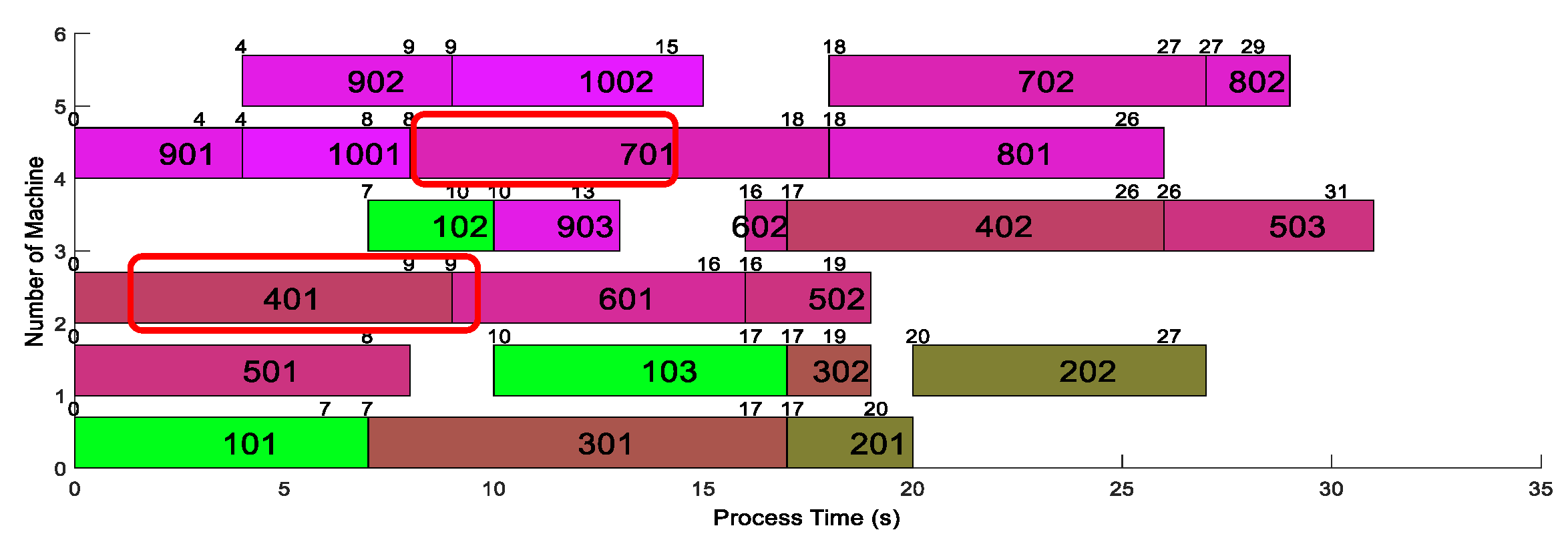
represents intercell job, denoted by jintercell, Mathematics 08 02225 i002 means current cell job, denoted by jintracell, S is the start processing time of the job in the result of intracell scheduling and E denotes the end time of job processing in the result of intracell scheduling.
Mathematics 08 02225 g008
Figure 9. The adjustment of intercell operation.
Mathematics 08 02225 g009
Figure 10. The adjustment of intracell operation.
Mathematics 08 02225 g010
Figure 11. Repeated adjustment for each cell until no new conflicts occur.
Mathematics 08 02225 g011
Figure 12. The Gantt chart of the two-stage solution.
Mathematics 08 02225 g012
Figure 13. Main effects plot. (a) Description of main effects plot for means; (b) Description of main effects plot for the SN ratios.
Mathematics 08 02225 g013
Figure 14. Comparison of the algorithms for cases of different sizes. (a) for cases 3 × 5 × 8 to 3 × 8 × 30. (b) for cases 4 × 5 × 8 to 4 × 8 × 30. (c) for cases 5 × 5 × 8 to 5 × 8 × 30. (d) for cases 6 × 5 × 8 to 6 × 8 × 30.
Mathematics 08 02225 g014aMathematics 08 02225 g014b
Figure 15. Comparison of SHHS and OHHS algorithms in terms of time consumption.
Mathematics 08 02225 g015
Table 1. Indices of variables used in problem statement and formulation.
Variables Meanings
J job set
E machine set
C cell set
M number of machines
N number of parts
K number of cells
m the index for machines m = 1,…M
j the index for jobs j = 1,…,N
k the index for cells k = 1,…K
i the sequence number of operations
oji the index for operations oji = 1,…Oj
Oj total operation number of jobs
Pjim the processing time of operation oji on machine m
tjkk the transportation time of job j from cell k to k
Cji the completion time of operation oji
xjim=1, if operation oji is required processing on machine m; 0, otherwise
yjit=1, if the start time of oji is t; 0, otherwise
zmm=1, if the equipment m and m’ is in the same cell; 0, otherwise
RD relative deviation
Bi the value gained by each algorithm for each problem
B the best solution found by all algorithms
Table 2. A sample example.
MachinesJobsCell of Machine
P1P2P3P4P5P6P7P8P9P10
M17310 1
M2772 8 1
M3 937 2
M43 951 3 2
M5 108443
M6 92563
process route1,4,21,21,23,42,3,43,45,65,65,6,45,6
cell of job1112223333
The unit of processing time of the jobs is second.
Table 3. The range of random cases.
CellsMachines in Each CellParts in Each Cell
358
4612
5720
6830
Table 4. Factors and their levels.
FactorLevel
12345
HMS1020304050
HMCR0.80.850.90.951
PAR0.050.10.150.20.25
Table 5. The orthogonal array L25(53) and experimental results of 3 × 5 × 8.
TestFactor
HMSHMCRPARValue
1100.800.05111
2100.850.10108
3100.900.15111
4100.950.20104
5101.000.25110
6200.800.10108
7200.850.15105
8200.900.20109
9200.950.25110
10201.000.05107
11300.800.15112
12300.850.20112
13300.900.25108
14300.950.05109
15301.000.10111
16400.800.20104
17400.850.25110
18400.900.05109
19400.950.10111
20401.000.15108
21500.800.25104
22500.850.05109
23500.900.10108
24500.950.15108
25501.000.20110
Table 6. Experimental result.
Instance
(c × m × p)
Two-Stage SolutionOverall Solution
SHHSSHGASHPSOOHHSOHGAOHPSO
ValueRDValueRDValueRDValueRDValueRDValueRD
3 × 5 × 81070.001150.071110.041100.031180.101140.07
3 × 5 × 121480.001770.201600.081570.061620.091510.02
3 × 5 × 202350.002580.102430.032460.052480.062390.02
3 × 5 × 303520.014040.153500.003550.013990.143530.01
3 × 6 × 81230.031230.031210.011220.021240.031200.00
3 × 6 × 121510.001870.241650.091700.131750.161560.03
3 × 6 × 202610.002770.072600.002600.002870.102610.00
3 × 6 × 303850.004210.103840.003910.024550.183910.02
3 × 7 × 81320.021480.151310.021300.011390.081290.00
3 × 7 × 121730.051910.161640.001820.112010.231730.05
3 × 7 × 202860.003010.052860.002960.033210.122960.03
3 × 7 × 304180.004580.104280.024240.014940.184340.04
3 × 8 × 81300.001580.221360.051460.121420.091390.07
3 × 8 × 121860.002180.171880.012040.102210.192020.09
3 × 8 × 203200.003610.133210.003270.023580.123260.02
3 × 8 × 304560.004800.054570.004670.024620.014660.02
4 × 5 × 81120.041190.101090.011120.041120.041080.00
4 × 5 × 121590.071570.051520.021560.051550.041490.00
4 × 5 × 202300.002710.182360.032440.062810.222500.09
4 × 5 × 303440.003770.103590.053430.004010.173580.04
4 × 6 × 81210.121380.281080.001260.171300.201140.06
4 × 6 × 121740.071750.071630.001770.091730.061660.02
4 × 6 × 202630.002930.112720.032670.022930.112760.05
4 × 6 × 303780.004220.123800.013940.044600.223960.05
4 × 7 × 81360.051300.001300.001370.051470.131310.01
4 × 7 × 121810.032010.151750.001960.122060.181900.09
4 × 7 × 203040.033340.133210.082960.003310.123130.06
4 × 7 × 304020.004880.214140.034270.064670.164390.09
4 × 8 × 81380.001660.201420.031500.091490.081460.06
4 × 8 × 121850.002270.231960.062150.162270.232050.11
4 × 8 × 203170.003550.123190.013290.043550.123270.03
4 × 8 × 304460.005060.134470.004650.045160.164640.04
5 × 5 × 81190.061260.131140.021170.041150.031120.00
5 × 5 × 121560.031710.131510.001590.051610.071540.02
5 × 5 × 202420.002860.182480.022570.062750.142630.09
5 × 5 × 303540.003960.123540.003630.034130.173630.03
5 × 6 × 81260.041260.041210.001290.071370.131250.03
5 × 6 × 121650.001820.101710.041670.011920.161730.05
5 × 6 × 202670.002940.102780.042730.023110.162830.06
5 × 6 × 303890.014420.154070.063850.004290.114030.05
5 × 7 × 81410.041470.081380.011390.021450.071360.00
5 × 7 × 121990.082180.182120.151850.002200.191980.07
5 × 7 × 202960.013350.152920.003060.053140.083020.03
5 × 7 × 304430.014580.054500.034380.004630.064450.02
5 × 8 × 81490.031820.261440.001550.081670.161500.04
5 × 8 × 122030.002360.162120.042100.032330.152190.08
5 × 8 × 203180.033540.153350.083090.003630.173260.06
5 × 8 × 304690.014960.074750.024650.005140.114710.01
6 × 5 × 81090.001270.171180.081190.091170.071100.01
6 × 5 × 121520.001840.211530.011620.071830.201610.06
6 × 5 × 202460.002690.092580.052530.032940.202650.08
6 × 5 × 303660.004050.113780.033670.003970.083790.04
6 × 6 × 81300.001540.181310.011310.011370.051320.02
6 × 6 × 121730.002000.161840.061750.011990.151860.08
6 × 6 × 202840.002990.062850.012830.003240.142840.00
6 × 6 × 304060.004330.074080.004100.014660.154120.01
6 × 7 × 81400.001510.081410.011420.011520.091430.02
6 × 7 × 121990.022140.102050.051950.002210.132010.03
6 × 7 × 202970.003370.133020.023040.023350.133090.04
6 × 7 × 304380.015020.154560.054350.004920.134530.04
6 × 8 × 81520.001740.141590.051520.001670.101590.05
6 × 8 × 122090.022300.122050.002230.092390.172200.07
6 × 8 × 203370.073530.123580.143150.003410.083360.07
6 × 8 × 304890.035030.065000.054750.005130.084860.02
averge 0.02 0.13 0.03 0.04 0.14 0.05
The red font means the best value found by all algorithms for each instance.
Publisher’s Note: MDPI stays neutral with regard to jurisdictional claims in published maps and institutional affiliations.

