Interference among Multiple Vibronic Modes in Two-Dimensional Electronic Spectroscopy

Abstract

Vibronic coupling between electronic and vibrational states in molecules plays a critical role in most photo-induced phenomena. Many key details about a molecule’s vibronic coupling are hidden in linear spectroscopic measurements, and therefore nonlinear optical spectroscopy methods such as two-dimensional electronic spectroscopy (2D ES) have become more broadly adopted. A single vibrational mode of a molecule leads to a Franck–Condon progression of peaks in a 2D spectrum. Each peak oscillates as a function of the waiting time, and Fourier transformation can produce a spectral slice known as a ‘beating map’ at the oscillation frequency. The single vibrational mode produces a characteristic peak structure in the beating map. Studies of single modes have limited utility, however, because most molecules have numerous vibrational modes that couple to the electronic transition. Interactions or interference among the modes may lead to complicated peak patterns in each beating map. Here, we use lineshape-function theory to simulate 2D ES arising from a system having multiple vibrational modes. The simulations reveal that the peaks in each beating map are affected by all of the vibrational modes and therefore do not isolate a single mode, which was anticipated.

1. Introduction

Scientists have several distinct interpretations of the term “vibronic coupling” [1,2]. The textbook molecular understanding [3] is that the electronic ($\left|\psi \right.〉$) and vibrational ($\left|\varphi \right.〉$) degrees of freedom in a molecule are separated to construct total molecular eigenfunctions having product-state form, $\left|\Phi \right.〉=\left|\psi \right.〉\otimes \left|\varphi \right.〉$. This leads to the ubiquitous displaced harmonic oscillator model and its accompanying Franck–Condon progression of peaks in linear absorption and fluorescence spectra [4]. In the conjugate view, vibronic coupling leads to the ultrafast modulation of a molecule’s electronic energy gap, $E_{\mathrm{eg}}\left(t\right)$. Using these complementary views, researchers have shown that vibronic coupling plays a key role in numerous photophysical, photochemical, and photobiological phenomena. Examples include singlet exciton fission [5,6], oxygenic photosynthesis [7], light-harvesting in biological [8,9,10,11,12] and synthetic [13,14,15] systems, and nonadiabatic transformations [16,17,18,19]. These studies have relied upon transient absorption and other four-wave mixing spectroscopy techniques.

Two-dimensional electronic spectroscopy (2D ES) is the ultimate four-wave mixing spectroscopy method because it can provide maximum resolution of the underlying nonlinear optical signal pathways [20,21,22,23]. In the most prevalent implementation of 2D ES measurements, three femtosecond laser pulses focus on a sample, from which they produce a four-wave mixing signal, which is a laser beam emitted by the sample that is subsequently detected by a spectrometer [24]. Heterodyning with a weak local-oscillator reference pulse allows researchers to extract both amplitude and phase information from the intensity-level measurement via the spectral interferometry method [25]. 2D ES is analogous to many more common methods from 2D nuclear magnetic resonance [26], and indeed the two techniques have similar interpretations regarding diagonal and cross peaks. Furthermore, 2D ES is equivalent to spectrally resolved transient absorption spectroscopy with the additional benefit of resolution of excitation frequencies [27]. In contrast to spectrally resolved transient absorption spectroscopy, however, 2D ES does not suffer from a time-frequency bandwidth constraint because the excitation frequency resolution arises from varying the time interval between the two pump pulses and a subsequent Fourier transformation.

The study of vibronic coupling using 2D ES dates back to some of the earliest 2D ES method-development research efforts of the late 1990s and early 2000s [28,29,30,31]. Since that time, numerous research groups have continued to pursue theoretical and experimental studies [32,33,34,35,36,37,38,39,40]. The result of these research efforts is that 2D ES measurements can be conducted with ultrabroad bandwidths adequate to resolve the complete manifold of vibronic peaks, allowing 2D ES to begin to be used as a mechanistic tool for photochemical reactions [41].

2D ES signals can be described theoretically using a perturbative treatment of the nonlinear optical signal [20]. In this method, the electronic system has a linear coupling to a manifold of harmonic oscillators to represent the surrounding solvent. The solvent causes dynamic fluctuations of the system’s electronic energy gap, and these fluctuations are captured mathematically by a lineshape function, $g\left(t\right)$, which is inserted into each third-order response function, $R^{\left(3\right)}({\tau }_1,{\tau }_2,{\tau }_3)$, to model the nonlinear optical signal that is measured in the laboratory. The lineshape function modulates the electronic transition during the three time intervals—${\tau }_1$, ${\tau }_2$, and ${\tau }_3$—between the laser pulse interactions. This general approach has been used to model a variety of four-wave mixing signals including transient absorption and two-pulse photon echo, among others [42]. Indeed many 2D ES studies have used this theoretical approach [32,43,44,45,46]. Despite this large body of literature, the interaction among multiple vibronic modes in 2D ES measurements has been observed [7,12,47,48,49], but not studied in detail. Therefore, in this contribution, we examine explicitly how multiple vibrational modes influence any given beating map constructed from a sequence of 2D spectra, in a context without the many possible nuclear modes and extensive coupling interactions that often obscure this relationship in laboratory measurements. The findings reveal that beating maps—although created by isolating the oscillations at a specific frequency during the waiting time interval—are indeed influenced by all of the vibrational modes of the system.

2. Results and Discussion

2.1. Theory: 2D ES Simulations

We aim to model the optical response of a molecular system due to excitation by light, which usually takes the form of laser pulses in the case of 2D ES. We therefore use a two-level electronic system as depicted in Figure 1 to describe the sample molecule, with the initial system in the ground state, $|g\rangle$. Franck–Condon excitation enables electronic transitions between $|g\rangle$ and the displaced excited state, $|e\rangle$, which are separated by a (thermally-averaged) energy gap with a frequency of ${\omega }_{eg}$. Solving for the first-order optical response function produces the linear spectrum resulting from excitation of the system, which can be conveniently described by the lineshape of the spectrum [20]. The absorption and fluorescence spectra, respectively, are given by,

$${\sigma }_{\mathrm{abs}}\left(\omega \right)=\frac{1}{\pi }\mathrm{Re}\left[{\int }_0^{\infty }{\mathrm{e}}^{i(\omega -{\omega }_{eg})t-\mathrm{g}\left(t\right)}dt\right],$$

(1)

$${\sigma }_{\mathrm{fluor}}\left(\omega \right)=\frac{1}{\pi }\mathrm{Re}\left[{\int }_0^{\infty }{\mathrm{e}}^{i(\omega -{\omega }_{eg}+2\lambda )t-{\mathrm{g}}^{*}\left(t\right)}dt\right],$$

(2)

where $i=\sqrt{-1}$. Here, $g\left(t\right)$ is the function for the line-broadening component of the lineshape, and $\lambda$ is a coupling strength parameter, sometimes referred to as the reorganization energy [50]. In Equation (2), the factor $2\lambda$ produces a redshift of the fluorescence peak with respect to the absorption peak, also known as the Stokes shift [20].

To simulate a 2D electronic spectrum, we calculate the third-order nonlinear optical response as a function of the three time intervals, ${\tau }_1$, ${\tau }_2$, and ${\tau }_3$. From the second-order cumulant expansion, we obtain the conventional third-order response functions,

$$\begin{array}{cc}\hfill R_1^{\left(3\right)}({\tau }_1,{\tau }_2,{\tau }_3)& ={\mathrm{e}}^{-i{\omega }_{eg}({\tau }_1+{\tau }_3)}\times {\mathrm{e}}^{-g\left({\tau }_1\right)-g^{*}\left({\tau }_2\right)-g^{*}\left({\tau }_3\right)+g({\tau }_1+{\tau }_2)+g^{*}({\tau }_2+{\tau }_3)-g({\tau }_1+{\tau }_2+{\tau }_3)},\hfill \\ \hfill R_2^{\left(3\right)}({\tau }_1,{\tau }_2,{\tau }_3)& ={\mathrm{e}}^{i{\omega }_{eg}({\tau }_1-{\tau }_3)}\times {\mathrm{e}}^{-g^{*}\left({\tau }_1\right)+g\left({\tau }_2\right)-g^{*}\left({\tau }_3\right)-g^{*}({\tau }_1+{\tau }_2)-g({\tau }_2+{\tau }_3)+g^{*}({\tau }_1+{\tau }_2+{\tau }_3)},\hfill \\ \hfill R_3^{\left(3\right)}({\tau }_1,{\tau }_2,{\tau }_3)& ={\mathrm{e}}^{i{\omega }_{eg}({\tau }_1-{\tau }_3)}\times {\mathrm{e}}^{-g^{*}\left({\tau }_1\right)+g^{*}\left({\tau }_2\right)-g\left({\tau }_3\right)-g^{*}({\tau }_1+{\tau }_2)-g^{*}({\tau }_2+{\tau }_3)+g^{*}({\tau }_1+{\tau }_2+{\tau }_3)},\hfill \\ \hfill R_4^{\left(3\right)}({\tau }_1,{\tau }_2,{\tau }_3)& ={\mathrm{e}}^{-i{\omega }_{eg}({\tau }_1+{\tau }_3)}\times {\mathrm{e}}^{-g\left({\tau }_1\right)-g\left({\tau }_2\right)-g\left({\tau }_3\right)+g({\tau }_1+{\tau }_2)+g({\tau }_2+{\tau }_3)-g({\tau }_1+{\tau }_2+{\tau }_3)}.\hfill \end{array}$$

(3)

Both the linear and nonlinear response functions include the lineshape function, $g\left(t\right)$, which takes the general expression [20],

$$g\left(t\right)=\frac{2\lambda k_{B}T}{\hslash }{\int }_0^t{\int }_0^{{\tau }_2}{M}^{\prime }\left({\tau }_1\right)d{\tau }_{2}d{\tau }_1-i\lambda {\int }_0^t\left[1-M^{″}\left(\tau \right)\right]d\tau .$$

(4)

$M\left(t\right)$ represents the electronic frequency correlation function, an analytic expression for incorporation into the nonlinear response functions.

The correlation functions represent the model system and incorporate the necessary components for vibronic coupling. The electronic transitions induced by optical excitation also involve transitions between the many vibrational (sub-)levels within each electronic level—vibronic coupling refers to this coupled relationship between electronic transitions and nuclear vibrational motion. We apply the Brownian oscillator model for the correlation function to incorporate the vibrational modes of both the molecular sample and its surrounding solvent. In this context, a nuclear vibration within a molecule acts as a coherent harmonic mode, which can be modeled as an underdamped Brownian oscillator [20,51]. We use the following correlation function for an underdamped oscillator with frequency ${\omega }_0$:

$$M_{\mathrm{vib}}\left(t\right)={\mathrm{e}}^{-\gamma t/2}\left[\cos \left({\overline{\omega }}_{0}t\right)+\left(\frac{\gamma }{2{\overline{\omega }}_0}\right)\sin \left({\overline{\omega }}_{0}t\right)\right].$$

(5)

Here, $\gamma$ is a vibrational relaxation rate parameter. Relaxation yields the reduced vibrational frequency, ${\overline{\omega }}_0$, of the original nuclear mode with frequency ${\omega }_0$:

$${\overline{\omega }}_0=\sqrt{{\omega }_0^2-{\gamma }^2/4}.$$

(6)

In practice, the solvent surrounding the sample molecule also contributes nuclear vibrations that influence the total spectroscopic response. Transfer of vibrational energy from the primary nuclear mode to the vibrations of the surrounding solvent promotes relaxation and dephasing of the nuclear oscillation. To incorporate these effects on the optical response, we model the solvent as a group of low-frequency, overdamped Brownian oscillators [20,50]:

$$M_{\mathrm{solv}}\left(t\right)={\mathrm{e}}^{-{\gamma }_{\mathrm{s}}t/2}\left(1+\frac{{\gamma }_{\mathrm{s}}t}{2}\right).$$

(7)

In this correlation function, the parameter ${\gamma }_{\mathrm{s}}$ represents the vibrational relaxation due to coupling to the solvent. Therefore, evaluating Equation (4) with the correlation functions for the nuclear modes (5) and solvent oscillations (7) yields their corresponding lineshape functions [50]:

$$\begin{array}{cc}\hfill g_{\mathrm{vib}}\left(t\right)& =\frac{\lambda {\mathrm{e}}^{-\gamma t/2}}{\beta \hslash {\overline{\omega }}_0{\left({\gamma }^2+4{\overline{\omega }}_0^2\right)}^2}[4{\mathrm{e}}^{\gamma t/2}{\overline{\omega }}_0\left(2{\gamma }^2(\gamma t-3)+8{\overline{\omega }}_0^2(\gamma t+1)+i\beta \hslash \gamma ({\gamma }^2+4{\overline{\omega }}_0^2)\right)\hfill \\ \hfill & +4{\overline{\omega }}_0\left(6{\gamma }^2-8{\overline{\omega }}_0^2-i\beta \hslash \gamma ({\gamma }^2+4{\overline{\omega }}_0^2)\right)\cos \left({\overline{\omega }}_{0}t\right)\hfill \\ \hfill & +\left(4\gamma ({\gamma }^2-12{\overline{\omega }}_0^2)-i\beta \hslash ({\gamma }^4-16{\overline{\omega }}_0^4)\right)\sin \left({\overline{\omega }}_{0}t\right)],\hfill \end{array}$$

(8)

$$\begin{array}{cc}\hfill g_{\mathrm{solv}}\left(t\right)& =\frac{4{\lambda }_{\mathrm{s}}}{\beta \hslash {\gamma }_{\mathrm{s}}^2}\left({\mathrm{e}}^{-{\gamma }_{\mathrm{s}}t/2}({\gamma }_{\mathrm{s}}t+6)+2{\gamma }_{\mathrm{s}}t-6\right)+\frac{i{\lambda }_{\mathrm{s}}}{{\gamma }_{\mathrm{s}}}\left(4-{\mathrm{e}}^{{\gamma }_{\mathrm{s}}t/2}({\gamma }_{\mathrm{s}}t+4)\right),\hfill \end{array}$$

(9)

where we have set $\beta =1/\left(k_{B}T\right)$ consistent with convention. These lineshape functions arise from a displaced harmonic oscillator model in which the frequencies of the ground and excited electronic states are identical and the Condon approximation is used. Furthermore, the model itself is widely used but has some physical flaws discussed by others [31,52] that make it a tractable theoretical model but prevent it from being used to make direct comparison to measured spectra. Lastly, the total lineshape function is the sum of the lineshapes for the discrete nuclear modes, indexed by n, and the solvent:

$$g\left(t\right)=\sum _n{g}_{\mathrm{vib},n}\left(t\right)+g_{\mathrm{solv}}\left(t\right).$$

(10)

The complete lineshape function $g\left(t\right)$ is used to evaluate the desired spectrum for the system. For example, the total $g\left(t\right)$ can be inserted into the third-order response functions from Equations (3) to compute the 2D spectrum. Evaluation over the ${\tau }_1$ and ${\tau }_3$ ranges followed by Fourier transformation produces the 2D spectrum across the ${\omega }_1$ (excitation frequency) and ${\omega }_3$ (detection frequency) axes, at a specific ${\tau }_2$ time that has elapsed since excitation of the sample with the pump laser pulses. A subsequent Fourier transform over a sequence of 2D spectra for varying ${\tau }_2$ values produces a 3D spectrum [53], and slicing through the 3D spectrum at a specific ${\omega }_2$ value produces a so-called ‘beating map’ of the oscillation amplitude and phase at this frequency [7,34,54]. Peaks arising in the beating maps indicate electronic transitions that induce oscillations at the ${\omega }_2$ frequency—therefore, selecting ${\omega }_2={\omega }_0$ means that, if peaks appear in the beating map, some will be spaced apart with a distance equivalent to ${\omega }_2$ corresponding to the frequency gap of vibrational transitions occurring in addition to the electronic transition. Prior studies of beating maps have not specifically examined the peak patterns that result when $n>1$ for the underdamped vibrational modes, likely because the anticipated result is that each beating map would isolate the contribution of the vibrations at that specified frequency. However, as seen in Figures 4 and 5 in Ref. [55] and in Figures 3 and S5 of Ref. [56], peaks do appear in beating maps at spacings other than the selected ${\omega }_2$ value. In this work, we examine this effect in detail by comparing beating maps computed using single-mode and multiple-mode systems that share vibrational frequencies.

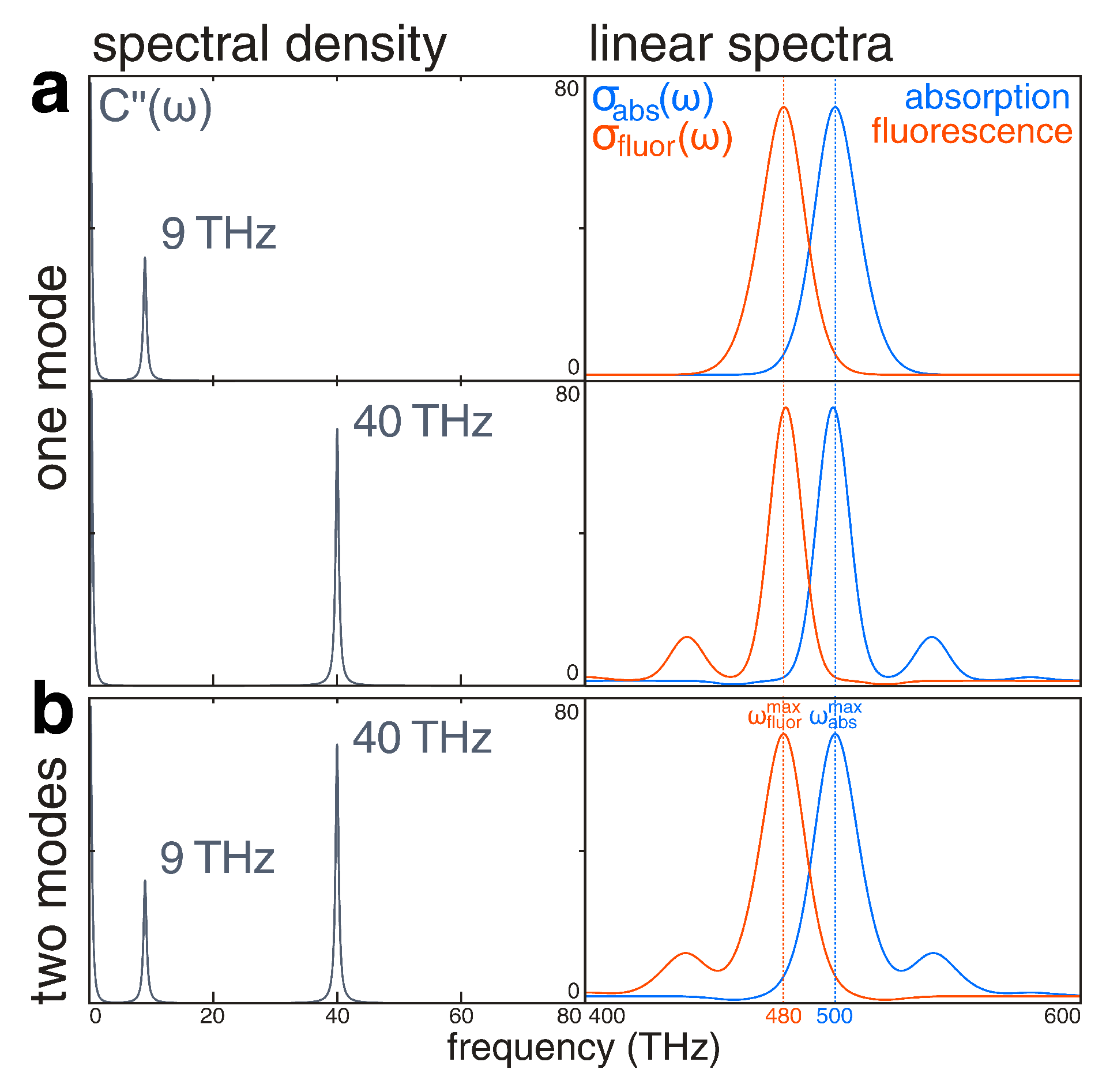
2.2. Linear Response: Spectral Density and Absorption and Fluorescence Spectra

We selected vibrational frequencies of 9 THz and 40 THz as nuclear modes, and examined the spectra produced by the individual modes and the combination of both modes using the theoretical methods described above. Importantly, we selected the mode frequencies to be neither factors nor multiples of each other to distinguish their spectral peaks: This avoids misidentification of any potential overtone peaks from one mode as peaks due to interference between two modes. We also implemented an energy gap between the ground and excited electronic states with frequency ${\omega }_{eg}=500$ THz, used a temperature high enough to satisfy the high-temperature limit [29], and applied consistent solvent parameters ${\lambda }_{\mathrm{s}}=$ 60 THz and ${\gamma }_{\mathrm{s}}=$ 2 THz to maintain the extent of homogeneous broadening and relaxation across all simulations [57].

First, we computed the linear response functions and produced 1D absorption and fluorescence spectra from the lineshapes in Equations (1) and (2). The spectral density, $C^{″}\left(\omega \right)$, is the 1D total correlation function in the frequency domain [20]. As shown in Figure 2, the amplitude of the spectral density is centered at the frequency of the nuclear mode(s), ${\omega }_0$, selected in each simulation. The Ohmic solvent contribution is visible at frequencies less than 5 THz. Figure 2 also shows the absorption and fluorescence spectra obtained from the 1D lineshapes for each simulation, with the maximum absorption frequency and the maximum fluorescence frequency separated by a Stokes shift of $2\lambda \equiv 20$ THz in all simulations, which we kept consistent through our choice of parameter values.

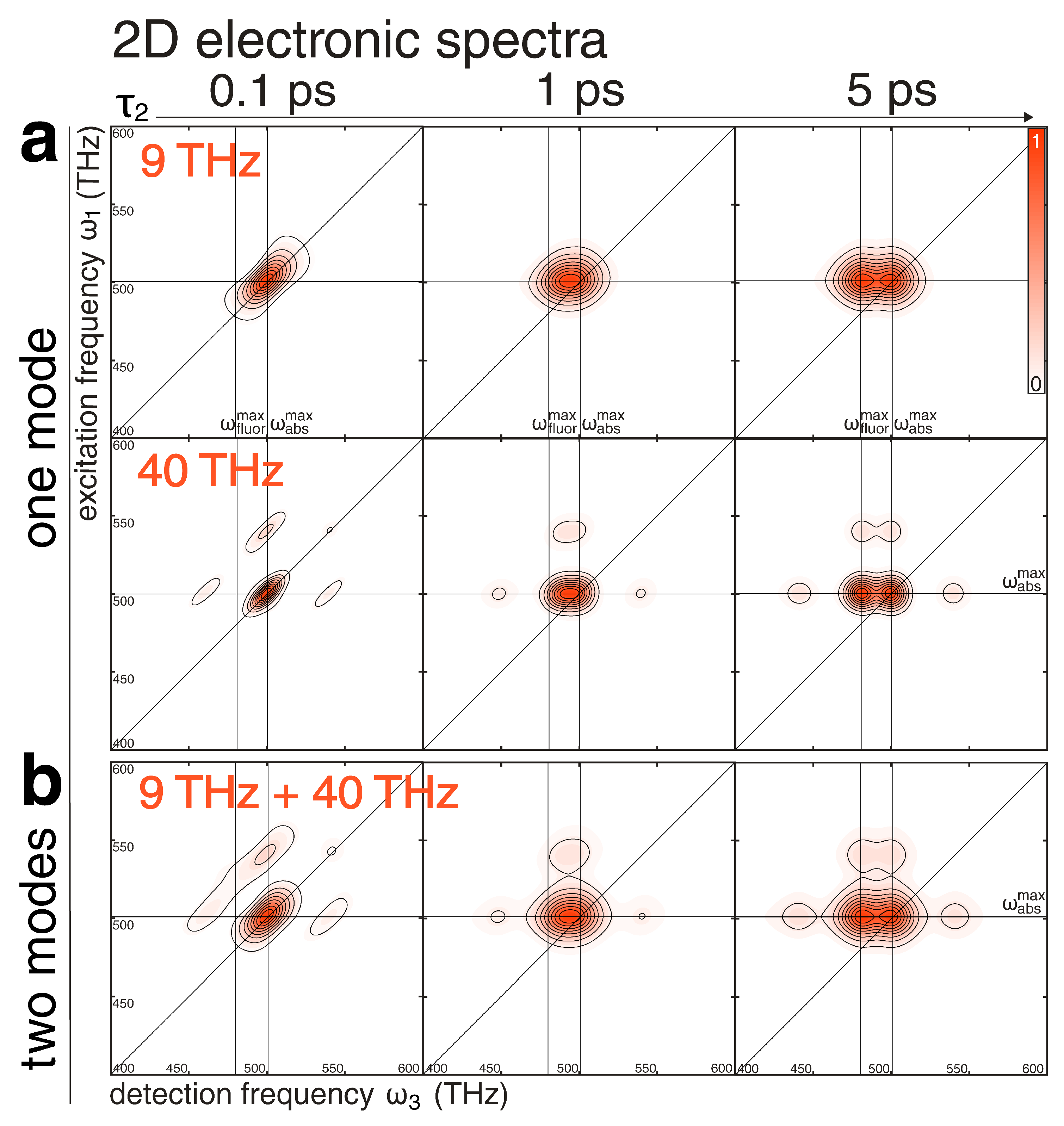
2.3. Nonlinear Response: 2D Electronic Spectra

Next, we present the 2D electronic spectra for the same single-mode and multi-mode systems described above, which are shown in Figure 3. As expected, at early ${\tau }_2$ time points (≲1 ps) after simulated pulsed excitation, the 2D spectra show a single positive peak that is elongated along the diagonal. The elongated, ellipse-shaped peak results from the line-broadening included in $g\left(t\right)$, and is a typical feature observed in experimental spectra at early times due to spectral diffusion [58]. By 1 ps, the diagonal line-broadening has diminished and the main peak has dispersed. As relaxation occurs, another peak composed of the stimulated emission signal splits from the main ground-state bleach peak, while moving from the maximum absorption frequency toward the maximum fluorescence frequency, which is redshifted from the maximum absorption by the Stokes shift. In all simulations, relaxation completes by 5 ps, as evidenced by the separation of the two peaks by the full Stokes shift with the ground-state bleach signal remaining at the maximum absorption frequency and the stimulated emission signal shifted to the maximum fluorescence frequency along the axis of detection (${\omega }_3$).

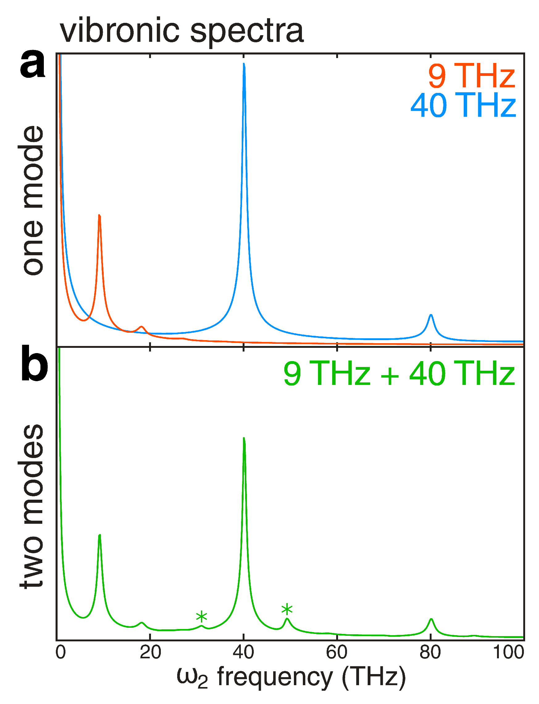
2.4. Vibronic Spectra and Beating Maps from 3D Electronic Spectra

Finally, we examine the spectroscopic signatures of vibronic coupling by assessing 1D vibronic spectra, and beating maps measured at the frequencies of the simulated nuclear modes. A vibronic spectrum is obtained by taking the sum of the 3D spectral data in the frequency domain along the ${\omega }_1$ and ${\omega }_3$ axes, which yields a plot of spectral amplitude versus ${\omega }_2$ frequency. As shown in Figure 4, a vibronic spectrum reveals the frequencies at which the vibrational wavepacket oscillates in the electronic states during time period ${\tau }_2$. Peaks indicate the frequencies at which vibrational transitions occur as a result of the optical excitation, with the peak intensities being determined by the coupling strength, $\lambda$. As expected, in simulations of one nuclear mode at 9 THz or 40 THz, the resulting vibronic spectra are dominated by a single main peak at the mode frequency ${\omega }_0$ (Figure 4a). Notably, both spectra simulated with one mode show a clear additional peak that is much smaller in amplitude and located at a frequency of $2{\omega }_0$. This peak corresponds to the overtone of the nuclear mode. When the system is simulated with two nuclear modes, the vibronic spectrum contains both primary peaks at their mode frequencies, the individual overtones, and combination-band peaks that were not present in the spectra of the individual modes (Figure 4b). The combination-band peaks have amplitudes on the same scale as the overtones and appear at 49 THz, corresponding to the sum of the two mode frequencies, and 31 THz, corresponding to their difference. The appearance of the combination-band peaks indicates that the vibrational wavepacket dynamics occur along both vibrational coordinates simultaneously, and that signatures of this complicated oscillatory motion should also appear in the 2D beating maps.

To further examine the origin of the combination-band peaks, we performed a series of simulations in which we held the parameters of the solvent and 40 THz mode constant but varied the coupling strength, $\lambda$, of the 9 THz mode. We quantified the relative intensity by extracting the intensity of the sum and difference frequency peaks in the 1D vibronic spectra and normalizing them to the intensity of the 40 THz peak. Based on a series of simulations in which $\lambda$ for the 9 THz mode varied from 0.4× to 1.8× its original value, we observed that a greater coupling strength enhances the intensity of the combination-band peaks. As follows, we surmise that increasing any component of the total coupling strength parameter will increase the intensity of any spectral signatures of vibronic coupling in the beating maps as well.

Next, we investigate the vibronic coupling in more detail by examining two-dimensional beating maps, which are slices of the 3D spectrum at selected ${\omega }_2$ frequencies where peaks arise from electronic transitions that involve vibrational transitions occurring at this ${\omega }_2$ frequency. Simulations of one nuclear mode display spectroscopic signal in the beating map magnitude (Figure 5a) measured at the ${\omega }_2$ frequency that matches the nuclear mode frequency, ${\omega }_0$. All the maps presented here show clear signatures of oscillations of the vibrational modes as a result of the optical excitation, indicating vibronic coupling between the electronic transition and the nuclear modes. Furthermore, the beating maps show unique spectroscopic signatures for the different individual modes. As expected, the peaks appear with spacings that correspond to their nuclear mode frequency: For the 40 THz mode, all the peaks are spaced 40 THz apart in the ${\omega }_3$ direction, and along the ${\omega }_1$ axis they are also 40 THz apart, while the two rows of peaks on either side of the frequency of maximum absorption are 40 THz away from this frequency, where a node is located. Similarly in the beating map of the 9 THz mode, a node is also found at approximately the frequency of maximum absorption along ${\omega }_1$, with the main peak located 9 THz above it. The beating maps from single-mode simulations reveal multiple broad peaks, which, comparing to the respective 2D spectra in Figure 3, indicate that the oscillations occur across the entirety of the peaks. Furthermore, the horizontal node at the excitation frequency corresponding to ${\omega }_{\mathrm{abs}}^{\max }$ indicates that peaks above and below this value oscillate out of phase.

In simulations of a system with two nuclear modes, the resulting beating maps (Figure 5b) also show clear evidence of vibronic coupling, yet are strikingly different from those of the same modes studied individually. Notably, two-mode beating maps seem to share some spectral features with the beating map of one individual nuclear mode, and some with the beating map of the other nuclear mode. The two-mode beating maps contain a combination of the peaks of their two individual modes, and this can be observed at ${\omega }_2$ frequencies equal to either of the two nuclear mode frequencies: The beating map of two modes at 9 THz and 40 THz (Figure 5b) shows significant oscillatory signal when examined at both ${\omega }_2=9$ THz and ${\omega }_2=40$ THz. In addition, both of these two-mode beating maps are noticeably different from the corresponding one-mode beating maps (Figure 5a), 9 THz at ${\omega }_2=9$ THz, and 40 THz at ${\omega }_2=40$ THz. Furthermore, we find peak spacings that correspond to both nuclear mode frequencies in the 9 THz + 40 THz beating maps. In the beating map measured at ${\omega }_2=9$ THz, the two peaks above the frequency of maximum absorption are 40 THz apart along the ${\omega }_1$ axis, and the displacement of the three peaks along the ${\omega }_3$ axis is 49 THz, corresponding to the combination of both modes. In the beating map at ${\omega }_2=40$ THz, we observe peak spacings of 31 THz, corresponding to the difference between the two modes, and 18 THz along the ${\omega }_1$ axis, and both 31 THz and 49 THz along the ${\omega }_3$ axis. Clearly, as observed in the vibronic spectra as combination-band peaks, there is also evidence of the oscillations of both modes present in the beating maps, measured at either frequency. Overall, these results indicate that the spectral features of multiple nuclear modes contribute additional signal arising from interference to the 2D electronic spectra.

An additional observation is that the beating maps from the same two-mode simulation vary distinctly when observed at the different ${\omega }_2$ frequencies of the two modes. Again demonstrated in Figure 5, the two-mode beating map with 9 THz and 40 THz modes, for example, is more similar to the one-mode beating map of the 9 THz mode when observed at ${\omega }_2=$ 9 THz, but retains more of the spectral signatures of the individual 40 THz mode beating map when observed at ${\omega }_2=$ 40 THz. This is logical based on the assumption that beating maps should isolate only the oscillations contributed by the specified ${\omega }_2$ frequency. However, the variance of the beating maps with multiple modes from the beating map of a single mode at the same ${\omega }_2$ frequency demonstrates that the oscillations corresponding to this frequency are not completely isolated—this indicates that interactions between different modes are also evident in beating maps.

To understand the origin of these interactions, we can re-examine the expressions for $g\left(t\right)$ and the response functions, from Equations (8) and (3). The response functions include many terms, but the terms most relevant to the interesting peaks in the beating maps are the oscillatory terms including cosine and sine functions [51], contributed from the expression for $g_{\mathrm{vib},\mathrm{n}}\left(t\right)$ as $\cos \left({\overline{\omega }}_{0,n}t\right)+\sin \left({\overline{\omega }}_{0,n}t\right)$. Because the response functions always involve the exponent of $g\left(t\right)$, when there are multiple modes present, this yields terms of the form ${\mathrm{e}}^{\cos \left({\overline{\omega }}_{0,a}t\right)\cos \left({\overline{\omega }}_{0,b}t\right)}$ for the cosine term, and the parallel expression for the sine term. Using standard trigonometric identities, these terms can be recast in terms of the sum and difference frequencies. For example, $2\cos \left({\overline{\omega }}_{0,a}t\right)\cos \left({\overline{\omega }}_{0,b}t\right)=\cos \left[({\overline{\omega }}_{0,a}-{\overline{\omega }}_{0,b})t\right]+\cos \left[({\overline{\omega }}_{0,a}+{\overline{\omega }}_{0,b})t\right]$. The presence of both the sum and difference of the two modes in the response functions leads directly to the generation of the combination bands in the vibronic spectra and to the interference and mixing between oscillatory signals observed in the beating maps of two nuclear modes. The occurrence of overtones and combination bands as a result of vibrational coherences between multiple fundamental modes is well-documented in vibrational spectroscopy [59,60]. Interactions between coupled vibrations have been demonstrated to produce combinations of the frequencies and new cross peaks in other nonlinear spectroscopies as well [61,62,63,64]. Overall, the various couplings and coherences can be revealed as additional signals and peak splittings in multidimensional spectroscopy techniques, such as the beating map measurements demonstrated here. The transformation of 2D spectra into beating maps provides more detailed information in multidimensional electronic spectroscopy, and reveals mixed oscillatory signals arising from all nuclear modes that are vibronically-coupled to electronic transitions.

Finally, it is worth envisioning extending these results using a more physically accurate model. In the lineshape-function model used here, the vibrational frequencies are the same in the ground and excited electronic states. In real molecules, however, the normal vibrational modes of the excited and ground states can be slightly different because the bonds have different force constants. This is known to affect the vibronic structure that is observable in linear absorption and fluorescence spectra [65,66]. Due to completeness, one can write a transformation matrix between the two normal-mode bases. Such a matrix is known as a Duschinksy rotation matrix [67]. This means, for example, that one could write a normal vibrational mode of the excited electronic state as a linear combination of some or all of the normal vibrational modes of the ground electronic state. This effect has been studied in the context of time-resolved four-wave mixing measurements previously [68], and it is intriguing to consider how this effect could be incorporated into the lineshape-function model and what effect it would have. The main expected difference is that each fundamental peak in the vibronic spectrum would become a doublet, one frequency for each electronic state. The relative intensities would be related to the coupling strengths. This increase in total number of peaks would then lead to additional interference terms. We anticipate that the Duschinksy effect could be incorporated into this model using an extended method developed by Tanimura and Mukamel [69] and recently used by our group to model Herzberg–Teller coupling in 2D ES beating maps [45].

3. Conclusions

In this article, we have simulated 2D electronic spectra and the beating maps resulting from a system with multiple nuclear modes. The interactions between nuclear modes in 2D ES have not been investigated in detail in previous work, although their spectral effects have been observed in laboratory measurements. We demonstrate that beating maps, showing oscillatory signals occurring at the frequency (${\omega }_2$) at which the map is measured, do not isolate purely the oscillations corresponding to the ${\omega }_2$ frequency as might be expected. Instead, if there are multiple modes, interference between their oscillatory signals arises in the beating maps as combinations of the spectral signatures from the individual modes. This ability to resolve signals of vibrational coherence and vibronic coupling through 2D ES beating maps is relevant to most molecular systems, which usually have numerous vibrational modes, and especially to many-atom materials like crystalline solids, which will continue to be of interest for applications in semiconductors, quantum computers, and photovoltaics. Further extensions of this model to include additional electronic states or doubly excited electronic states would be relevant for studies of electronic energy-transfer or many-body interactions, respectively. In such cases, beating maps can be especially useful for deciphering the coupling interactions that are possible between multiple electronic and vibrational transitions. The spectral interferences observed in this work will be important for interpreting measurements of these systems, especially as multidimensional spectroscopy is used to study a wider range of samples and more complicated excited-state processes in the near future.

References

1. Fulton, R.L. Vibronic Interactions. The Adiabatic Approximation. J. Chem. Phys. 1972, 56, 1210–1218. [Google Scholar] [CrossRef]
2. Azumi, T.; Matsuzaki, K. What Does the Term “Vibronic Coupling” Mean? Photochem. Photobiol. 1977, 25, 315–326. [Google Scholar] [CrossRef]
3. McQuarrie, D.A.; Simon, J.D. Physical Chemistry: A Molecular Approach; University Science Books: Mill Valley, CA, USA, 1997. [Google Scholar]
4. McHale, J.L. Molecular Spectroscopy, 2nd ed.; CRC Press: Boca Raton, FL, USA, 2017. [Google Scholar]
5. Bakulin, A.A.; Morgan, S.E.; Kehoe, T.B.; Wilson, M.W.B.; Chin, A.W.; Zigmantas, D.; Egorova, D.; Rao, A. Real-time observation of multiexcitonic states in ultrafast singlet fission using coherent 2D electronic spectroscopy. Nat. Chem. 2015, 8, 16–23. [Google Scholar] [CrossRef] [Green Version]
6. Breen, I.; Tempelaar, R.; Bizimana, L.A.; Kloss, B.; Reichman, D.R.; Turner, D.B. Triplet separation drives singlet fission after femtosecond correlated triplet pair production in rubrene. J. Am. Chem. Soc. 2017, 139, 11745–11751. [Google Scholar] [CrossRef] [PubMed]
7. Fuller, F.D.; Pan, J.; Gelzinis, A.; Butkus, V.; Senlik, S.S.; Wilcox, D.E.; Yocum, C.F.; Valkunas, L.; Abramavicius, D.; Ogilvie, J.P. Vibronic coherence in oxygenic photosynthesis. Nat. Chem. 2014, 6, 706–711. [Google Scholar] [CrossRef] [PubMed]
8. Womick, J.M.; Moran, A.M. Vibronic Enhancement of Exciton Sizes and Energy Transport in Photosynthetic Complexes. J. Phys. Chem. B 2011, 115, 1347–1356. [Google Scholar] [CrossRef] [PubMed]
9. Womick, J.M.; West, B.A.; Scherer, N.F.; Moran, A.M. Vibronic effects in the spectroscopy and dynamics of C-phycocyanin. J. Phys. B At. Mol. Opt. Phys. 2012, 45, 154016. [Google Scholar] [CrossRef]
10. Richards, G.H.; Wilk, K.E.; Curmi, P.M.G.; Quiney, H.M.; Davis, J.A. Coherent Vibronic Coupling in Light-Harvesting Complexes from Photosynthetic Marine Algae. J. Phys. Chem. Lett. 2012, 3, 272–277. [Google Scholar] [CrossRef]
11. Singh, V.P.; Westberg, M.; Wang, C.; Dahlberg, P.D.; Gellen, T.; Gardiner, A.T.; Cogdell, R.J.; Engel, G.S. Towards quantification of vibronic coupling in photosynthetic antenna complexes. J. Chem. Phys. 2015, 142, 212446. [Google Scholar] [CrossRef] [Green Version]
12. Thyrhaug, E.; Tempelaar, R.; Alcocer, M.J.P.; Zidek, K.; Bina, D.; Knoester, J.; Jansen, T.L.C.; Zigmantas, D. Identification and characterization of diverse coherences in the Fenna–Matthews–Olson complex. Nat. Chem. 2018, 10, 780–786. [Google Scholar] [CrossRef]
13. Song, Y.; Clafton, S.N.; Pensack, R.D.; Kee, T.W.; Scholes, G.D. Vibrational coherence probes the mechanism of ultrafast electron transfer in polymer–fullerene blends. Nat. Commun. 2014, 5, 4933. [Google Scholar] [CrossRef] [PubMed] [Green Version]
14. Lenngren, N.; Abdellah, M.A.; Zheng, K.; Al-Marri, M.J.; Zigmantas, D.; Zidek, K.; Pullerits, T. Hot electron and hole dynamics in thiol-capped CdSe quantum dots revealed by 2D electronic spectroscopy. Phys. Chem. Chem. Phys. 2016, 18, 26199–26204. [Google Scholar] [CrossRef] [PubMed] [Green Version]
15. De Sio, A.; Lienau, C. Vibronic coupling in organic semiconductors for photovoltaics. Phys. Chem. Chem. Phys. 2017, 19, 18813. [Google Scholar] [CrossRef] [PubMed]
16. Meyer, H.D. A classical model of vibronic coupling: The ultrafast non-radiative decay via a conical intersection. Chem. Phys. 1983, 82, 199–205. [Google Scholar] [CrossRef]
17. Vos, M.H.; Rappaport, F.; Lambry, J.C.; Breton, J.; Martin, J.L. Visualization of Coherent Nuclear Motion in a Membrane Protein by Femtosecond Spectroscopy. Nature 1993, 363, 320–325. [Google Scholar] [CrossRef]
18. Peters, W.K.; Smith, E.R.; Jonas, D.M. Femtosecond Pump-Probe Polarization Spectroscopy of Vibronic Dynamics at Conical Intersections and Funnels. In Conical Intersections: Theory, Computation and Experiment; Advanced Series in Physical Chemistry; Domcke, W., Yarkony, D.R., Köppel, H., Eds.; World Scientific: Singapore, 2011; Volume 17. [Google Scholar]
19. Johnson, P.J.M.; Halpin, A.; Morizumi, T.; Prokhorenko, V.I.; Ernst, O.P.; Miller, R.J.D. Local Vibrational Coherences Drive the Primary Photochemistry of Vision. Nat. Chem. 2015, 7, 980–986. [Google Scholar] [CrossRef]
20. Mukamel, S. Principles of Nonlinear Optical Spectroscopy; Oxford University Press: New York, NY, USA, 1995. [Google Scholar]
21. Hamm, P.; Zanni, M.T. Concepts and Methods of 2D Infrared Spectroscopy; Cambridge University Press: Cambridge, UK, 2011. [Google Scholar] [CrossRef]
22. Brańczyk, A.M.; Turner, D.B.; Scholes, G.D. Crossing disciplines—A view on two-dimensional optical spectroscopy. Ann. Phys. 2013, 526, 31–49. [Google Scholar] [CrossRef] [Green Version]
23. Wright, J.C. Analytical chemistry, multidimensional spectral signatures, and the future of coherent multidimensional spectroscopy. Chem. Phys. Lett. 2016, 662, 1–13. [Google Scholar] [CrossRef] [Green Version]
24. Fuller, F.D.; Ogilvie, J.P. Experimental Implementations of Two-Dimensional Fourier Transform Electronic Spectroscopy. Ann. Rev. Phys. Chem. 2015, 66, 667–690. [Google Scholar] [CrossRef]
25. Lepetit, L.; Cheriaux, G.; Joffre, M. Linear Techniques of Phase Measurement by Femtosecond Spectral Interferometry for Application in Spectroscopy. J. Opt. Soc. Am. B 1995, 12, 2467–2474. [Google Scholar] [CrossRef]
26. Jonas, D.M. Optical Analogs of 2D NMR. Science 2003, 300, 1515–1517. [Google Scholar] [CrossRef] [PubMed]
27. Lewis, K.L.M.; Ogilvie, J.P. Probing Photosynthetic Energy and Charge Transfer with Two-Dimensional Electronic Spectroscopy. J. Phys. Chem. Lett. 2012, 3, 503–510. [Google Scholar] [CrossRef] [PubMed]
28. Hybl, J.D.; Albrecht, A.W.; Gallagher Faeder, S.M.; Jonas, D.M. Two-Dimensional Electronic Spectroscopy. Chem. Phys. Lett. 1998, 297, 307–313. [Google Scholar] [CrossRef] [Green Version]
29. Gallagher Faeder, S.M.; Jonas, D.M. Two-Dimensional Electronic Correlation and Relaxation Spectra: Theory and Model Calculations. J. Phys. Chem. A 1999, 103, 10489–10505. [Google Scholar] [CrossRef]
30. Hybl, J.D.; Albrecht Ferro, A.; Jonas, D.M. Two-Dimensional Fourier Transform Electronic Spectroscopy. J. Chem. Phys. 2001, 115, 6606–6622. [Google Scholar] [CrossRef]
31. Hybl, J.D.; Yannick, C.; Jonas, D.M. Peak Shapes in Femtosecond 2D Correlation Spectroscopy. Chem. Phys. 2001, 266, 295–309. [Google Scholar] [CrossRef]
32. Nemeth, A.; Milota, F.; Mancal, T.; Lukes, V.; Kauffmann, H.F.; Sperling, J. Vibronic modulation of lineshapes in two-dimensional electronic spectra. Chem. Phys. Lett. 2008, 459, 94–99. [Google Scholar] [CrossRef]
33. Milota, F.; Sperling, J.; Nemeth, A.; Mancal, T.; Kauffmann, H.F. Two-dimensional electronic spectroscopy of molecular excitons. Acc. Chem. Res. 2009, 42, 1364–1374. [Google Scholar] [CrossRef]
34. Turner, D.B.; Dinshaw, R.; Lee, K.K.; Belsley, M.S.; Wilk, K.E.; Curmi, P.M.G.; Scholes, G.D. Quantitative investigations of quantum coherence for a light-harvesting protein at conditions simulating photosynthesis. Phys. Chem. Chem. Phys. 2012, 14, 4857–4874. [Google Scholar] [CrossRef] [Green Version]
35. Chenu, A.; Christensson, N.; Kauffmann, H.F.; Mancal, T. Enhancement of Vibronic and Ground-State Vibrational Coherences in 2D Spectra of Photosynthetic Complexes. Sci. Rep. 2013, 3, 2029. [Google Scholar] [CrossRef] [Green Version]
36. Egorova, D. Oscillations in two-dimensional photo-echo signals of excitonic and vibronic systems: Stick-spectrum analysis and its computational verification. J. Chem. Phys. 2014, 140, 034314. [Google Scholar] [CrossRef] [PubMed]
37. Halpin, A.; Johnson, P.J.M.; Tempelaar, R.; Murphy, R.S.; Knoester, J.; Jansen, T.L.C.; Miller, R. Two-dimensional spectroscopy of a molecular dimer unveils the effects of vibronic coupling on exciton coherences. Nat. Chem. 2014, 6, 196–201. [Google Scholar] [CrossRef] [PubMed]
38. Spokoyny, B.; Harel, E. Mapping the Vibronic Structure of a Molecule by Few-Cycle Continuum Two-Dimensional Spectroscopy in a Single Pulse. J. Phys. Chem. Lett. 2014, 5, 2808–2814. [Google Scholar] [CrossRef] [PubMed]
39. Albert, J.; Falge, M.; Gomez, S.; Sola, I.R.; Hildenbrand, H.; Engel, V. Communication: Vibrational and vibronic coherences in the two dimensional spectroscopy of coupled electron-nuclear motion. J. Chem. Phys. 2015, 143, 041102. [Google Scholar] [CrossRef] [PubMed] [Green Version]
40. Bizimana, L.A.; Brazard, J.; Carbery, W.P.; Gellen, T.; Turner, D.B. Resolving Molecular Vibronic Structure using High-Sensitivity Two-Dimensional Electronic Spectroscopy. J. Chem. Phys. 2015, 143, 164203. [Google Scholar] [CrossRef] [PubMed]
41. Carbery, W.P.; Pinto-Pacheco, B.; Buccella, D.; Turner, D.B. Resolving the Fluorescence Quenching Mechanism of an Oxazine Dye Using Ultrabroadband Two-Dimensional Electronic Spectroscopy. J. Phys. Chem. A 2019, 123, 5072–5080. [Google Scholar] [CrossRef] [PubMed]
42. Ohta, K.; Larsen, D.S.; Yang, M.; Fleming, G.R. Influence of intramolecular vibrations in third-order, time-domain resonant spectroscopies. II. Numerical calculations. J. Chem. Phys. 2001, 114, 8020–8039. [Google Scholar] [CrossRef]
43. Nemeth, A.; Milota, F.; Mancal, T.; Lukes, V.; Hauer, J.; Kauffmann, H.F.; Sperling, J. Vibrational wave packet induced oscillations in two-dimensional electronic spectra. I. Experiments. J. Chem. Phys. 2010, 132, 184514. [Google Scholar] [CrossRef] [Green Version]
44. Fidler, A.F.; Harel, E.; Engel, G.S. Dissecting Hidden Couplings Using Fifth-Order Three-Dimensional Electronic Spectroscopy. J. Phys. Chem. Lett. 2010, 1, 2876–2880. [Google Scholar] [CrossRef]
45. Bizimana, L.A.; Carbery, W.P.; Gellen, T.; Turner, D.B. Signatures of Herzberg–Teller coupling in three-dimensional electronic spectroscopy. J. Chem. Phys. 2017, 146, 084311. [Google Scholar] [CrossRef]
46. Bizimana, L.A.; Epstein, J.; Brazard, J.; Turner, D.B. Conformational Homogeneity in the Pr Isomer of Phytochrome Cph1. J. Phys. Chem. B 2017, 121, 2622–2630. [Google Scholar] [CrossRef] [PubMed]
47. Milota, F.; Prokhorenko, V.I.; Mancal, T.; von Berlepsch, H.; Bixner, O.; Kauffmann, H.F.; Hauer, J. Vibronic and Vibrational Coherences in Two-Dimensional Electronic Spectra of Supramolecular J-Aggregates. J. Phys. Chem. A 2013, 117, 6007–6014. [Google Scholar] [CrossRef] [PubMed]
48. Tempelaar, R.; Jansen, T.L.C.; Knoester, J. Vibrational Beatings Conceal Evidence of Electronic Coherence in the FMO Light-Harvesting Complex. J. Phys. Chem. B 2014, 118, 12865–12872. [Google Scholar] [CrossRef] [PubMed]
49. Policht, V.R.; Niedringhaus, A.; Ogilvie, J.P. Characterization of Vibrational Coherence in Monomeric Bacteriochlorophyll a by Two-Dimensional Electronic Spectroscopy. J. Phys. Chem. Lett. 2018, 9, 6631–6637. [Google Scholar] [CrossRef] [PubMed]
50. Butkus, V.; Valkunas, L.; Abramavicius, D. Molecular Vibrations-Induced Quantum Beats in Two-Dimensional Electronic Spectroscopy. J. Chem. Phys. 2012, 137, 044513. [Google Scholar] [CrossRef] [PubMed] [Green Version]
51. Mancal, T.; Nemeth, A.; Milota, F.; Lukes, V.; Hauer, J.; Kauffmann, H.F.; Sperling, J. Vibrational wave packet induced oscillations in two-dimensional electronic spectra. II. Theory. J. Chem. Phys. 2010, 132, 184515. [Google Scholar] [CrossRef] [Green Version]
52. Gallagher Faeder, S.M. A Two-Dimensional Fourier Transform Spectroscopic Study of the Non-Equilibrium Solvation Dynamics of IR144 in Methanol. Ph.D. Thesis, University of Colorado, Boulder, CO, USA, 1999. [Google Scholar]
53. Turner, D.B.; Stone, K.W.; Gundogdu, K.; Nelson, K.A. Three-Dimensional Electronic Spectroscopy of Excitons in GaAs Quantum Wells. J. Chem. Phys. 2009, 131, 144510. [Google Scholar] [CrossRef]
54. Bašinskaitė, E.; Butkus, V.; Abramavicius, D.; Valkunas, L. Vibronic models for nonlinear spectroscopy simulations. Photosynth. Res. 2014, 121, 95–106. [Google Scholar] [CrossRef]
55. Gellen, T.A.; Lem, J.; Turner, D.B. Probing Homogeneous Line Broadening in CdSe Nanocrystals using Multidimensional Electronic Spectroscopy. Nano Lett. 2017, 17, 2809–2815. [Google Scholar] [CrossRef]
56. Bizimana, L.A.; Farfan, C.A.; Brazard, J.; Turner, D.B. E to Z Photoisomerization of Phytochrome Cph1Δ Exceeds the Born–Oppenheimer Adiabatic Limit. J. Phys. Chem. Lett. 2019, 10, 3550–3556. [Google Scholar] [CrossRef]
57. Butkus, V.; Valkunas, L.; Abramavicius, D. Vibronic phenomena and exciton-vibrational interference in two-dimensional spectra of molecular aggregates. J. Chem. Phys. 2014, 140. [Google Scholar] [CrossRef] [PubMed] [Green Version]
58. Roberts, S.T.; Loparo, J.J.; Tokmakoff, A. Characterization of Spectral Diffusion from Two-Dimensional Line Shapes. J. Chem. Phys. 2006, 125, 084502. [Google Scholar] [CrossRef] [PubMed]
59. Efremov, E.V.; Ariese, F.; Mank, A.J.G.; Gooijer, C. Strong Overtones and Combination Bands in Ultraviolet Resonance Raman Spectroscopy. Anal. Chem. 2006, 78, 3152–3157. [Google Scholar] [CrossRef] [PubMed]
60. De Souza, B.; Farias, G.; Neese, F.; Izsák, R. Efficient simulation of overtones and combination bands in resonant Raman spectra. J. Chem. Phys. 2019, 150. [Google Scholar] [CrossRef] [PubMed]
61. Khalil, M.; Tokmakoff, A. Signatures of vibrational interactions in coherent two-dimensional infrared spectroscopy. Chem. Phys. 2001, 266, 213–230. [Google Scholar] [CrossRef]
62. Nee, M.J.; Baiz, C.R.; Anna, J.M.; McCanne, R.; Kubarych, K.J. Multilevel vibrational coherence transfer and wavepacket dynamics probed with multidimensional IR spectroscopy. J. Chem. Phys. 2008, 129. [Google Scholar] [CrossRef]
63. Liang, K.K.; Villaeys, A.A. Anharmonicity and mode-mode coupling effects analyzed by four-wave-mixing photon-echo spectroscopy. Phys. Rev. A 2010, 82. [Google Scholar] [CrossRef]
64. Gaynor, J.D.; Khalil, M. Signatures of vibronic coupling in two-dimensional electronic-vibrational and vibrational-electronic spectroscopies. J. Chem. Phys. 2017, 147. [Google Scholar] [CrossRef]
65. Santoro, F.; Improta, R.; Lami, A.; Bloino, J.; Barone, V. Effective method to compute Franck–Condon integrals for optical spectra of large molecules in solution. J. Chem. Phys. 2007, 126. [Google Scholar] [CrossRef]
66. Niu, Y.; Peng, Q.; Deng, C.; Gao, X.; Shuai, Z. Theory of Excited State Decays and Optical Spectra: Application to Polyatomic Molecules. J. Phys. Chem. A 2010, 114, 7817–7831. [Google Scholar] [CrossRef]
67. Duschinsky, F.Z.D. Der Elektronenspektren mehratomiger Moleküle. Acta Physicochim. URSS 1937, 7, 551–566. [Google Scholar]
68. Fuji, T.; Saito, T.; Kobayashi, T. Dynamical observation of Duschinksy rotation by sub-5-fs real-time spectroscopy. Chem. Phys. Lett. 2000, 332, 324–330. [Google Scholar] [CrossRef]
69. Tanimura, Y.; Mukamel, S. Real-time path-integral approach to quantum coherence and dephasing in nonadiabatic transitions and nonlinear optical response. Phys. Rev. E 1993, 47, 118–136. [Google Scholar] [CrossRef] [PubMed]
Figure 1. Two-level system of harmonic oscillators used to model a sample with electronic states | g and | e (green) in the presence of a solvent environment (blue). Excitation induces an electronic transition (red) between | g and | e , which are separated by a frequency gap of ω e g . Nuclear modes, or vibrational transitions (light green) with characteristic frequencies indicated by ω 0 , also occur. Vibronic coupling takes place as coupling between the vibrational transitions and the electronic transition.
Mathematics 08 00157 g001
Figure 2. Spectral density, C ( ω ) (left panels), and linear spectra from absorption and fluorescence lineshapes, σ abs ( ω ) and σ fluor ( ω ) (right panels), calculated with (a) one mode with frequency ω 0 = 9 THz or 40 THz and (b) two modes with frequencies ω 0 = 9 THz + 40 THz. In the linear spectra, the frequency of maximum absorption ( ω abs max ) and the frequency of maximum fluorescence ( ω fluor max ) are labeled.
Mathematics 08 00157 g002
Figure 3. 2D electronic spectra shown at τ 2 time points of 0.1 ps, 1 ps, and 5 ps from simulations of (a) one mode with frequency ω 0 = 9 THz or 40 THz and (b) two modes with frequencies ω 0 = 9 THz + 40 THz. The horizontal line indicates the frequency of maximum absorption ( ω abs max ), and the vertical lines indicate both the frequency of maximum absorption ( ω abs max ) and the frequency of maximum fluorescence ( ω fluor max ). The diagonal line indicates where ω 1 = ω 3 , or excitation frequency is equivalent to detection (or emission) frequency.
Mathematics 08 00157 g003
Figure 4. Vibronic spectra showing total amplitude over ω 2 frequencies, obtained from 3D electronic spectra that were Fourier-transformed into the frequency domain. Total vibronic spectra are shown from simulations of (a) one mode with frequency ω 0 = 9 THz (red) or 40 THz (blue), and (b) two modes with frequencies ω 0 = 9 THz + 40 THz (green), where asterisks label the combination-band peaks at 31 THz and 49 THz.
Mathematics 08 00157 g004
Figure 5. Beating maps (magnitude) shown at ω 2 = 9 THz or 40 THz. Beating maps were obtained from 3D electronic spectra simulated using (a) one mode with frequency ω 0 = 9 THz or 40 THz, and (b) two modes with frequencies ω 0 = 9 THz + 40 THz.
Mathematics 08 00157 g005