Two Approaches to the Construction of Perturbation Bounds for Continuous-Time Markov Chains

Abstract

This paper is largely a review. It considers two main methods used to study stability and to obtain appropriate quantitative estimates of perturbations of (inhomogeneous) Markov chains with continuous time and a finite or countable state space. An approach is described to the construction of perturbation estimates for the main five classes of such chains associated with queuing models. Several specific models are considered for which the limit characteristics and perturbation bounds for admissible “perturbed” processes are calculated.

1. Introduction

In this paper, some topics are considered that are related to the stability of both homogeneous and non-homogeneous continuous-time Markov chains with respect to the perturbation of their intensities (infinitesimal characteristics). It is assumed that the evolution of the system under consideration is described by a Markov chain with the known state space, and it is the infinitesimal matrix that is given inexactly. Different classes of admissible perturbations can be considered. The “perturbed” infinitesimal matrix can be arbitrary, and the small deviation of its norm from that of the original matrix is assumed or it can be assumed that the structure of the infinitesimal matrix is known and only its elements are “perturbed” within the same structure. Below we will give a detailed description of these cases. In some papers it is assumed that the perturbations have a special form and, for example, are expanded in a power series of a small parameter. This assumption seems to be too restrictive and unrealistic.

The study of stability of characteristics of stochastic models has been actively developing since the 1970s [1,2,3]. At that time, Zolotarev proposed to treat limit theorems of probability theory as special stability theorems. Zolotarev created the theoretical foundation of the key method used within this approach, namely, the theory of probability metrics [4]. This approach assumes that statements establishing the convergence must be accompanied by statements establishing the convergence rate. Zolotarev called the conditions of convergence that simultaneously serve as convergence rate estimates “natural.” This approach was developed in the works of Zolotarev, Kalashnikov, Kruglov, Senatov, Yu, Korolev, Yu, Khokhlov, and their colleagues in the framework of international seminars on stability problems for stochastic models. This seminar was founded by Zolotarev in the early 1970s and still continues to hold its regular (as a rule, annual) international sessions (see the series of the proceedings of the seminar published as Springer Lecture Notes starting from [5] or as issues of the Journal of Mathematical Sciences). In particular, this approach proved to be very productive for the study of random sums in queueing theory, renewal theory, and the theory of branching processes [6].

Since the 1980s, the problems related to the estimation of stability of Markov chains with respect to perturbations of their characteristics have been thoroughly studied by Kartashov for homogeneous discrete-time chains with general state space and, in parallel, by Zeifman for inhomogeneous continuous-time chains within the seminar mentioned above (see [7,8,9]). In particular, a general approach for inhomogeneous continuous-time chains was developed in [9]. That paper was published in the proceedings of the seminar “Stability Problems for Stochastic Models” and dealt with both uniform and strong cases.

Later birth-death processes were considered in [10], and general properties and estimates for inhomogeneous finite chains were considered in [11]. The paper [12] was specially devoted to estimates for general birth-death processes, with the queueing system $M_t\left|M_t\right|N$ considered as an example. It should be mentioned that these papers were not noticed by Western authors. For example, in [13], it was stated that there were no papers on the stability of the (simplest stationary!!) system $M\left|M\right|1$. For the first time, we used the term “perturbation bounds” instead of “stability” in the paper [14] on the referee’s prompt. The same situation takes place with Kartashov’s papers cited above. The methods proposed in those papers seem to be used by most authors of subsequent studies in estimations of perturbations of discrete-time chains. Possibly, poor acquaintance with the early papers of Kartashov and Zeifman can be explained by the differences in terminology mentioned above: in the original (and foundational) papers, the term “stability” was used (in the proceedings of the seminar with the consonant appellation “Stability Problems for Stochastic Models”).

The present paper deals only with continuous-time chains, so the subsequent remarks mainly regard such a case.

Note that, to obtain explicit and exact estimates of the perturbation bounds of a chain, it is required to have estimates of the rate of convergence of the chain to its limit characteristics in the form of explicit inequalities. Moreover, the sharper the convergence rate estimates are, the more accurate the perturbation bounds are. These bounds can be more easily obtained for finite homogeneous Markov chains. Therefore, most publications concern this situation only (see, e.g., [15,16,17,18,19,20]). Thus, two main approaches can be highlighted.

The first of them can be used for the case of weak ergodicity of a chain in the uniform operator topology. The first bounds in this direction were obtained in [9]. The principal progress related to the replacement of the constant S with $logS$ in the bound was implemented in [17] and continued in Mitrophanov’s papers [18,19,20] for the case of homogeneous chains and then in [14,21] and in the subsequent papers of these authors for the inhomogeneous chains. The contemporary state of affairs in this field and new applied problems related to the link between convergence rate and perturbation bounds in the “uniform” case were described in [22]. In some recent papers, uniform perturbation bounds of homogeneous Markov chains were studied by the techniques of stochastic differential equations (see, for instance, [23] and the references therein).

The second approach is used in the case where the uniform ergodicity is not assured, which is typical for the processes most interesting from a practical viewpoint. For example, birth-death processes used for modeling queueing systems, and real processes in biology, chemistry, and physics, as a rule, are not uniformly ergodic.

Following the ideas of Kartashov (see a detailed description in [24]), most authors use the probability methods to study ergodicity and perturbation bounds of stationary chains (with a finite, countable, or general state space) in various norms [13,25,26]. For a wide class of (mainly) stationary discrete-time chains, a close approach was considered in [27] and more recent papers [28,29,30,31,32,33,34,35,36,37,38].

In the works of the authors of the present paper, perturbation bounds for non-stationary finite or infinite continuous-time chains were studied by other methods.

The first papers dealing with non-stationary queueing models appeared in the 1970s (see [39,40], and the more recent paper [41]). Moreover, as far back as the year in which [42] was published, it was noted that it is principally possible to use the logarithmic matrix norm for the study of the convergence rate of continuous-time Markov chains. The corresponding general approach employing the theory of differential equations in Banach spaces was developed in a series of papers by the authors of the present paper(see a detailed description in [43,44]). In [9] (see also [10,11]), a method for the study of perturbation bounds for the vector of state probabilities of a continuous-time Markov chain with respect to the perturbations of infinitesimal characteristics of the chain in the total variation norm ($l_1$-norm) was proposed. The paper [12] contained a detailed study of the stability of essentially non-stationary birth-death processes with respect to conditionally small perturbations. Convergence rate estimates in terms of weight norms, and hence the corresponding bounds for new classes of Markov chains, were considered in [45,46,47,48].

In the present paper, both approaches are considered along with the classes of inhomogeneous Markov chains, for which at least one of these approaches yields reasonable perturbation bounds for basic probability characteristics.

The paper is organized as follows. In Section 2, basic notions and preliminary results are introduced. In Section 3, general theorems on perturbation bounds are considered. Section 4 contains convergence rate estimates and perturbation bounds for basic classes of the chains under consideration. Finally, in Section 5, some special queueing models are studied.

2. Basic Notions and Preliminaries

Let $X=X\left(t\right)$, $t\ge 0$, be, in general, an inhomogeneous continuous-time Markov chain with a finite or countable state space $E_S=0,1,\dots ,S$, $S\le \infty$. The transition probabilities for $X=X\left(t\right)$ will be denoted $p_{ij}(s,t)=Pr\left\{X\left(t\right)=j\left|X\left(s\right)=i\right.\right\}$, $i,j\ge 0,0\le s\le t$. Let $p_i\left(t\right)=Pr\left\{X\left(t\right)=i\right\}$ be the state probabilities of the chain and $\mathbf{p}\left(t\right)={\left(p_0\left(t\right),p_1\left(t\right),\dots \right)}^T$ be the corresponding vector of state probabilities. In what follows, it is assumed that

$$Pr\left\{X\left(t+h\right)=j|X\left(t\right)=i\right\}=$$

$$=\left\{\begin{array}{cc}{q}_{ij}\left(t\right)h+{\alpha }_{ij}\left(t,h\right),\hfill & \mathrm{if}j\ne i\hfill \\ 1-{\displaystyle \sum _{k\ne i}{q}_{ik}\left(t\right)h+{\alpha }_i\left(t,h\right)},\hfill & \mathrm{if}j=i\hfill \end{array}\right.$$

(1)

where all ${\alpha }_i(t,h)$ are $o\left(h\right)$ uniformly in i, that is, ${sup}_i\left|{\alpha }_i(t,h)\right|=o\left(h\right)$.

As usual, we assume that, if a chain is inhomogeneous, then all the infinitesimal characteristics (intensity functions) $q_{ij}\left(t\right)$ are integrable in t on any interval $[a,b]$, $0\le a\le b$.

Let $a_{ij}\left(t\right)=q_{ji}\left(t\right)$ for $j\ne i$ and $a_{ii}\left(t\right)=-{\sum }_{j\ne i}{a}_{ji}\left(t\right)=-{\sum }_{j\ne i}{q}_{ij}\left(t\right)$.

Further, to provide the possibility to obtain more evident estimates, we will assume that

$$|a_{ii}\left(t\right)|\le L<\infty$$

(2)

for almost all $t\ge 0$.

The state probabilities then satisfy the forward Kolmogorov system

$$\frac{d\mathbf{p}}{dt}=A\left(t\right)\mathbf{p}\left(t\right)$$

(3)

where $A\left(t\right)=Q^T\left(t\right)$, and $Q\left(t\right)$ is the infinitesimal matrix of the process.

Let $\parallel ·\parallel$ be the usual $l_1$-norm, i.e. $\parallel \mathbf{x}\parallel =\sum |x_i|$, and $\parallel B\parallel ={sup}_j{\sum }_i\left|b_{ij}\right|$ for $B={\left(b_{ij}\right)}_{i,j=0}^{\infty }$. Denote $\mathsf{\Omega }=\left\{\mathbf{x}:\mathbf{x}\in l_1^{+}\&\parallel \mathbf{x}\parallel =1\right\}$. Therefore,

$$\parallel A\left(t\right)\parallel =2\underset{k}{sup}\left|a_{kk}\left(t\right)\right|\le 2L$$

for almost all $t\ge 0$, and we can apply the results of [49] to Equation (3) in the space $l_1$. Namely, in [49] it was shown that the Cauchy problem for Equation (3) has a unique solution for an arbitrary initial condition. Moreover, if $\mathbf{p}\left(s\right)\in \mathsf{\Omega }$, then $\mathbf{p}\left(t\right)\in \mathsf{\Omega }$, for any $0\le s\le t$ and any initial condition $\mathbf{p}\left(s\right)$.

Let $p_0\left(t\right)=1-{\sum }_{i\ge 1}{p}_i\left(t\right)$.

Put $\mathbf{z}={\left(p_1,p_2,\dots \right)}^T$.

Therefore, from Equation (3), we obtain the equation

$$\frac{d\mathbf{z}}{dt}=B\left(t\right)\mathbf{z}\left(t\right)+\mathbf{f}\left(t\right),$$

(4)

where $\mathbf{f}={\left(a_{10},a_{20},\dots \right)}^T$,

$$B=\left(\begin{array}{ccccc}{a}_{11}-a_{10}& a_{12}-a_{10}& \dots & a_{1r}-a_{10}& \dots \\ a_{21}-a_{20}& a_{22}-a_{20}& \dots & a_{2r}-a_{20}& \dots \\ a_{31}-a_{30}& a_{32}-a_{30}& \dots & a_{3r}-a_{30}& \dots \\ \dots \\ a_{r1}-a_{r0}& a_{r2}-a_{r0}& \dots & a_{rr}-a_{r0}& \dots \\ \dots \dots \dots \end{array}\right),$$

(5)

where all expressions depend on t.

By $\overline{X}=\overline{X}\left(t\right)$, we will denote the “perturbed” Markov chain with the same state space, state probabilities ${\overline{p}}_i\left(t\right)$, transposed infinitesimal matrix $\overline{A}\left(t\right)={\left({\overline{a}}_{ij}\left(t\right)\right)}_{i,j=0}^{\infty }$, and so on, and the “perturbations” themselves, that is, the differences between the corresponding “perturbed” and original characteristics will be denoted by ${\widehat{a}}_{ij}\left(t\right)$, $\widehat{A}\left(t\right)$.

Let $E(t,k)=E\left\{X\left(t\right)\left|X\left(0\right)=k\right.\right\}$. Recall that a Markov chain $X\left(t\right)$ is weakly ergodic if $\parallel {\mathbf{p}}^{*}\left(t\right)-{\mathbf{p}}^{**}\left(t\right)\parallel \to 0$ as $t\to \infty$ for any initial condition, and it has the limiting mean $\varphi \left(t\right)$ if $\left|E\right(t,k)-\varphi (t\left)\right|\to 0$ as $t\to \infty$ for any k.

Now we briefly describe the main classes of the chains under consideration. The details concerning the first four classes can be found in [47,50].

Case 1.

Let $a_{ij}\left(t\right)=0$ for all $t\ge 0$ if $|i-j|>1$, and $a_{i,i+1}\left(t\right)={\mu }_{i+1}\left(t\right)$, $a_{i+1,i}\left(t\right)={\lambda }_i\left(t\right)$. This is an inhomogeneous birth-death process (BDP) with the intensities ${\lambda }_i\left(t\right)$ (of birth) and ${\mu }_{i+1}\left(t\right)$ (of death) correspondingly.

Case 2.

Now let $a_{ij}\left(t\right)=0$ for $i<j-1$, $a_{i+k,i}\left(t\right)=a_k\left(t\right)$ for $k\ge 1$, and $a_{i,i+1}\left(t\right)={\mu }_{i+1}\left(t\right)$. This chain describes, for instance, the number of customers in a queueing system in which the customers arrive in groups, but are served one by one (in this case, $a_k\left(t\right)$ is the arrival intensity of a group of k customers, and ${\mu }_i\left(t\right)$ is the service intensity of the ith customer). The simplest models of this type were considered in [51] (see also [47,50]).

Case 3.

Let $a_{ij}\left(t\right)=0$ for $i>j+1$, $a_{i,i+k}\left(t\right)=b_k\left(t\right)$, $k\ge 1$, and $a_{i+1,i}\left(t\right)={\lambda }_i\left(t\right)$. This situation occurs in modeling queueing systems with the arrivals of single customers and group service.

Case 4.

Let $a_{i+k,i}\left(t\right)=a_k\left(t\right)$, $a_{i,i+k}\left(t\right)=b_k\left(t\right)$ for $k\ge 1$. This process appears in the description of a system with group arrival and group service, for earlier studies see [46,52,53].

Case 5.

Consider a Markov chain with “catastrophes” used for modeling of some queueing systems (see, e.g., [14,54,55,56,57,58]). Here the intensities have a general form, whereas a single (although substantial) restriction consists in that the zero state is attainable from any other state, and the corresponding intensities $q_{k,0}\left(t\right)=a_{0,k}\left(t\right)$ for $k\ge 1$ are called the intensities of catastrophes.

Now consider the following example illustrating some specific features of the problem under consideration.

Example 1

([14]). Consider a homogeneous BDP (Class I) with the intensities ${\lambda }_k\left(t\right)=1$, ${\mu }_k\left(t\right)=4$ for all t and k and denote by A the corresponding transposed intensity matrix. Therefore, as is known (see, e.g., [59]), the BDP is strongly ergodic and stable in the corresponding norm. On the other hand, take a perturbed process with the transposed infinitesimal matrix $\overline{A}=A+\widehat{A}$, where ${\widehat{a}}_{00}=-\epsilon$, ${\widehat{a}}_{k0}=\frac{\epsilon }{k(k+1)}$ for $k\ge 1$, and ${\widehat{a}}_{ij}=0$ for the other $i,j$. The perturbed Markov chain $\overline{X}\left(t\right)$ (describing the “M|M|c queue with mass arrivals when empty” (see [54,58,60])) is then not ergodic, since, from the condition $\overline{A}\overline{\mathbf{p}}=0$, it follows that the coordinates of the stationary distribution (if it exists) must satisfy the condition $4{\overline{p}}_{k+1}={\overline{p}}_k+{\overline{p}}_0\frac{\epsilon }{k+1}\ge {\overline{p}}_0\frac{\epsilon }{k+1}$, which is impossible.

As has already been noted, the (upper) bounds of perturbations are closely connected with the (correspondingly, upper) estimates for the convergence rate (see also the two next sections). On the other side, it is also possible to construct important lower estimates of the rate of convergence provided that the influence of the initial conditions cannot fade too rapidly (see [61]). It turns out that it is principally impossible to construct lower bounds for perturbations. Indeed, if we consider the same BDP and, as a perturbed BDP, choose a BDP with the intensities ${\overline{\lambda }}_k\left(t\right)=1+\epsilon$, ${\overline{\mu }}_k\left(t\right)=4(1+\epsilon )$, then the stationary distribution for the perturbed process will be the same as that for the original BDP for any positive $\epsilon$.

3. General Theorems Concerning Perturbation Bounds

First consider uniform bounds that provide the first approach to perturbation estimation. This approach is applied to uniformly ergodic Markov chains and the study of stability of the state probability vector. The most important class of such processes is that of Markov chains on finite state space, both homogeneous and inhomogeneous.

Theorem 1.

Let the Markov chain $X\left(t\right)$ be exponentially weakly ergodic; that is, for any initial conditions ${\mathbf{p}}^{*}\left(s\right)\in \mathsf{\Omega }$, ${\mathbf{p}}^{**}\left(s\right)\in \mathsf{\Omega }$ and any $s\ge 0$, $t\ge s$, there holds the inequality

$$\parallel {\mathbf{p}}^{*}\left(t\right)-{\mathbf{p}}^{**}\left(t\right)\parallel \le 2c{e}^{-b(t-s)}.$$

(6)

Therefore, for the perturbations small enough ($\widehat{A}\left(t\right)\le \epsilon$ for almost all $t\ge 0$), the perturbed chain $\overline{X}\left(t\right)$ is also exponentially weakly ergodic, and the following perturbation bound takes place:

$$\underset{t\to \infty }{lim\; sup}\parallel \mathbf{p}\left(t\right)-\overline{\mathbf{p}}\left(t\right)\parallel \le \frac{\left(1+log(c/2)\right)\epsilon }{b}.$$

(7)

For the proof, we will use the approach proposed in [17] and modified in [21] for the inhomogeneous case, see also [14]. Let

$$\beta (t,s)=\underset{\parallel \mathbf{v}\parallel =1,\sum v_i=0}{sup}\parallel U\left(t\right)\mathbf{v}\parallel =\frac{1}{2}\underset{i,j}{sup}\sum _k|p_{ik}(t,s)-p_{jk}(t,s)|.$$

(8)

Therefore,

$$\parallel \mathbf{p}\left(t\right)-\overline{\mathbf{p}}\left(t\right)\parallel \le \beta (t,s)\parallel \mathbf{p}\left(s\right)-\overline{\mathbf{p}}\left(s\right)\parallel +{\int }_s^t\parallel \widehat{A}\left(u\right)\parallel \beta (u,s)du.$$

(9)

Moreover,

$$\beta (t,s)\le 1,\beta (t,s)\le \frac{c}{2}{e}^{-b(t-s)},0\le s\le t.$$

(10)

Hence,

$$\parallel \mathbf{p}\left(t\right)-\overline{\mathbf{p}}\left(t\right)\parallel \le$$

$$\left\{\begin{array}{cc}\parallel \mathbf{p}\left(s\right)-\overline{\mathbf{p}}\left(s\right)\parallel +(t-s)\epsilon ,\hfill & if0<t-s<\frac{1}{b}ln\frac{c}{2},\hfill \\ \frac{c}{2}{e}^{-b(t-s)}\parallel \mathbf{p}\left(s\right)-\overline{\mathbf{p}}\left(s\right)\parallel +\frac{1}{b}(ln\frac{c}{2}+1-c{e}^{-b(t-s)})\epsilon ,\hfill & ift-s\ge \frac{1}{b}ln\frac{c}{2}\hfill \end{array}\right.$$

(11)

whence, as $t\to \infty$, we obtain Equation (7).

Corollary 1.

If under the conditions of Theorem 1 the Markov chain $X\left(t\right)$ has a finite state space, then both Markov chains $X\left(t\right)$ and $\overline{X}\left(t\right)$ have limit expectations and

$$|\varphi \left(t\right)-\overline{\varphi }\left(t\right)|\le \frac{1}{b}S\left(1+log(c/2)\right)\epsilon .$$

(12)

Now consider the second approach. Namely, we turn to weighted bounds. Such estimates can be applied to a wide class of Markov chains which are exponentially ergodic in some weighted norms. Moreover, as a rule, these estimates also allow one to study stability characteristics of the mathematical expectation for countable Markov chains, both homogeneous and inhomogeneous. Here we use the approach proposed in [9] (see also the detailed description in [43,44]).

Let $1\le d_1\le d_2\le \dots$,

$$D=\left(\begin{array}{cccc}{d}_1& d_1& d_1& \dots \\ 0& d_2& d_2& \dots \\ 0& 0& d_3& \dots \\ & \dots & \dots & \dots \end{array}\right).$$

(13)

Let $l_{1D}=\left\{\mathbf{z}={(p_1,p_2,\dots )}^T{:\parallel \mathbf{z}\parallel }_{1D}\equiv \parallel D\mathbf{z}\parallel <\infty \right\}$. Therefore, ${\parallel B\parallel }_{1D}=\parallel DB{D}^{-1}\parallel$. In addition, let ${\parallel \mathbf{p}\parallel }_{1D}={\parallel \mathbf{z}\parallel }_{1D}$.

Below we will assume that the following conditions hold:

$${\parallel B\left(t\right)\parallel }_{1D}\le \mathfrak{B}<\infty ,{\parallel \mathbf{f}\left(t\right)\parallel }_{1D}\le \mathfrak{f}<\infty$$

(14)

for almost all $t\ge 0$.

Recall that $X\left(t\right)$ is a $1D$-exponentially weakly ergodic Markov chain if

$$\parallel {\mathbf{p}}^{*}\left(t\right)-{\mathbf{p}}^{**}{\left(t\right)\parallel }_{1D}\le M{e}^{-a\left(t-s\right)}{\parallel {\mathbf{p}}^{*}\left(s\right)-{\mathbf{p}}^{**}\left(s\right)\parallel }_{1D}.$$

(15)

for some $M>0$, $a>0$ and any $s,t$: $t\ge s\ge 0$, any initial conditions ${\mathbf{p}}^{*}\left(s\right)\in l_{1D}$, ${\mathbf{p}}^{**}\left(s\right)\in l_{1D}$.

If one can choose ${\mathbf{p}}^{**}\left(t\right)=\pi$, then the chain is $1D$-exponentially strongly ergodic.

Let

$$\parallel B\left(t\right)-\overline{B}{\left(t\right)\parallel }_{1D}\le \left|\mathfrak{B}-\overline{\mathfrak{B}}\right|,{\parallel \mathbf{f}\left(t\right)-\overline{\mathbf{f}}\left(t\right)\parallel }_{1D}\le \left|\mathfrak{f}-\overline{\mathfrak{f}}\right|.$$

(16)

for almost all $t\ge 0$.

Theorem 2.

If a Markov chain $X\left(t\right)$ is $1D$-exponentially weakly ergodic, then $\overline{X}\left(t\right)$ is also $1D$-exponentially weakly ergodic and the following perturbation estimate in the $1D$-norm holds:

$$\begin{array}{c}\hfill \underset{t\to \infty }{lim\; sup}{\parallel \mathbf{p}\left(t\right)-\overline{\mathbf{p}}\left(t\right)\parallel }_{1D}\le \frac{M\left(M\left|\mathfrak{B}-\overline{\mathfrak{B}}\right|\mathfrak{f}+a\left|\mathfrak{f}-\overline{\mathfrak{f}}\right|\right)}{a\left(a-M\left|\mathfrak{B}-\overline{\mathfrak{B}}\right|\right)}.\end{array}$$

(17)

If $W={inf}_{i\ge 1}\frac{d_i}{i}>0$, then both chains $X\left(t\right)$ and $\overline{X}\left(t\right)$ have limiting means and

$$\begin{array}{c}\hfill \underset{t\to \infty }{lim\; sup}|\varphi \left(t\right)-\overline{\varphi }\left(t\right)|\le \frac{M\left(M\left|\mathfrak{B}-\overline{\mathfrak{B}}\right|\mathfrak{f}+a\left|\mathfrak{f}-\overline{\mathfrak{f}}\right|\right)}{Wa\left(a-M\left|\mathfrak{B}-\overline{\mathfrak{B}}\right|\right)}.\end{array}$$

(18)

Proof. 

The detailed consideration can be found in [44]. Here we only outline the scheme of reasoning. Let $V(t,s)$ and $\overline{V}(t,s)$ be the Cauchy operators for Equation (4) and for the corresponding “perturbed” equation, respectively. Therefore,

$${\parallel V(t,s)\parallel }_{1D}\le M{e}^{-a(t-s)},{\parallel \overline{V}(t,s)\parallel }_{1D}\le M{e}^{-\left(a-M\left|\mathfrak{B}-\overline{\mathfrak{B}}\right|\right)(t-s)}$$

(19)

for all $t\ge s\ge 0$. Therefore, rewriting Equation (4) as

$$\frac{d\mathbf{z}}{dt}=\overline{B}\left(t\right)\mathbf{z}\left(t\right)+\mathbf{f}\left(t\right)+\left(B\left(t\right)-\overline{B}\left(t\right)\right)\mathbf{z}\left(t\right),$$

(20)

after some algebra, we obtain the following inequality in the $1D$-norm:

$$∥\mathbf{z}\left(t\right)-\overline{\mathbf{z}}\left(t\right)∥\le {\int }_0^t\parallel \overline{V}(t,\tau )\parallel \left(\parallel B\left(\tau \right)-\overline{B}\left(\tau \right)\parallel \parallel \mathbf{z}\left(\tau \right)\parallel +\parallel \mathbf{f}\left(\tau \right)-\overline{\mathbf{f}}\left(\tau \right)\parallel \right)d\tau \le$$

$$\le {\int }_0^{t}M{e}^{-\left(a-M\left|\mathfrak{B}-\overline{\mathfrak{B}}\right|\right)(t-\tau )}\left(\left|\mathfrak{B}-\overline{\mathfrak{B}}\right|\parallel \mathbf{z}\left(\tau \right)\parallel +\left|\mathfrak{f}-\overline{\mathfrak{f}}\right|\right)d\tau .$$

(21)

On the other hand, ${\parallel \mathbf{z}\left(t\right)\parallel }_{1D}\le M{e}^{-at}{\parallel \mathbf{z}\left(0\right)\parallel }_{1D}+\frac{M}{a}\mathfrak{f}$, for any $0\le s\le t$. Hence, under any initial condition $\mathbf{z}\left(0\right)\in l_{1D}$, we obtain the following inequalities for the $1D$-norm:

$$∥\mathbf{z}\left(t\right)-\overline{\mathbf{z}}\left(t\right)∥\le M\left(\left|\mathfrak{B}-\overline{\mathfrak{B}}\right|\frac{M}{a}\mathfrak{f}+\left|\mathfrak{f}-\overline{\mathfrak{f}}\right|\right){\int }_0^t{e}^{-\left(a-M\left|\mathfrak{B}-\overline{\mathfrak{B}}\right|\right)(t-\tau )}d\tau +$$

$$+M{\int }_0^t{e}^{-\left(a-M\left|\mathfrak{B}-\overline{\mathfrak{B}}\right|\right)(t-\tau )}\left|\mathfrak{B}-\overline{\mathfrak{B}}\right|M{e}^{-a\tau }\parallel \mathbf{z}\left(0\right)\parallel d\tau \le$$

$$\le \frac{M\left(M\left|\mathfrak{B}-\overline{\mathfrak{B}}\right|\mathfrak{f}+a\left|\mathfrak{f}-\overline{\mathfrak{f}}\right|\right)}{a\left(a-M\left|\mathfrak{B}-\overline{\mathfrak{B}}\right|\right)}+o\left(1\right).$$

(22)

Therefore, the first assertion of the theorem is proved.

Therefore, the second assertion follows from the inequality ${\parallel \mathbf{z}\parallel }_{1E}\le W^{-1}{\parallel \mathbf{z}\parallel }_{1D}$ (see, e.g., [62]) and the estimate expressed by Equation (22), where $l_{1E}=\left\{z={(p_1,p_2,\dots )}^T{:\parallel z\parallel }_{1E}\equiv \sum n\left|p_n\right|<\infty \right\}$ □.

Remark 1.

A number of consequences of this statement can be formulated, for example,

$$\underset{t\to \infty }{lim\; sup}\parallel \mathbf{p}\left(t\right)-\overline{\mathbf{p}}\left(t\right)\parallel \le \frac{4M\left(M\left|\mathfrak{B}-\overline{\mathfrak{B}}\right|\mathfrak{f}+a\left|\mathfrak{f}-\overline{\mathfrak{f}}\right|\right)}{ad\left(a-M\left|\mathfrak{B}-\overline{\mathfrak{B}}\right|\right)},$$

(23)

which follows from

$$\parallel {\mathbf{p}}^{*}-{\mathbf{p}}^{**}\parallel \le 2\parallel {\mathbf{z}}^{*}-{\mathbf{z}}^{**}\parallel \le \frac{4}{d}{\parallel {\mathbf{z}}^{*}-{\mathbf{z}}^{**}\parallel }_{1D}.$$

(24)

The respective perturbation bounds can be formulated for strongly ergodic (for instance, homogeneous) Markov chains (see [44]).

Remark 2.

As shown in [44], the bounds presented in Theorem 2 and its corollaries are sufficiently sharp. Namely, in [44], we considered the queue-length process for the simplest ordinary $M/M/1$ queue and proved that the bounds established in Theorem 2 have the proper order.

4. Convergence Rate Estimates and Perturbation Bounds for Main Classes

For Markov chains of Classes 1–4, an important role is played by the matrix $B^{**}\left(t\right)=DB\left(t\right)D^{-1}$. To begin with, write out this matrix for each of these classes.

For Class 1, this matrix has the form

$B^{**}\left(t\right)=$

$$=\left(\begin{array}{ccccccc}-\left({\lambda }_0+{\mu }_1\right)& \frac{d_1}{d_2}{\mu }_1& 0& \cdots & 0& \cdots & \cdots \\ \frac{d_2}{d_1}{\lambda }_1& -\left({\lambda }_1+{\mu }_2\right)& \frac{d_2}{d_3}{\mu }_2& \cdots & 0& \cdots & \cdots \\ \ddots & \ddots & \ddots & \ddots & \ddots & \cdots \\ 0& \cdots & \cdots & \frac{d_r}{d_{r-1}}{\lambda }_{r-1}& -\left({\lambda }_{r-1}+{\mu }_r\right)& \frac{d_r}{d_{r+1}}{\mu }_r& \cdots \\ \cdots & \cdots & \cdots & \cdots & \cdots & \cdots & \cdots \end{array}\right)$$

(25)

in the case of a countable state space ($S=\infty$);

$B^{**}\left(t\right)=$

$$=\left(\begin{array}{ccccc}-\left({\lambda }_0+{\mu }_1\right)& \frac{d_1}{d_2}{\mu }_1& 0& \cdots & 0\\ \frac{d_2}{d_1}{\lambda }_1& -\left({\lambda }_1+{\mu }_2\right)& \frac{d_2}{d_3}{\mu }_2& \cdots & 0\\ \ddots & \ddots & \ddots & \ddots & \ddots \\ 0& \cdots & \cdots & \frac{d_S}{d_{S-1}}{\lambda }_{S-1}& -\left({\lambda }_{S-1}+{\mu }_S\right)\end{array}\right)$$

(26)

in the case of a finite state space ($S<\infty$).

For Class 2, this matrix has the form

$$B^{**}\left(t\right)=\left(\begin{array}{ccccc}{a}_{11}& \frac{d_1}{d_2}{\mu }_1& 0& \cdots & 0\\ \frac{d_2}{d_1}{a}_1& a_{22}& \frac{d_2}{d_3}{\mu }_2& \cdots & 0\\ \frac{d_3}{d_1}{a}_2& \frac{d_3}{d_2}{a}_1& a_{33}& \frac{d_3}{d_4}{\mu }_3& \cdots & \\ \ddots & \ddots & \ddots & \ddots & \ddots \\ \ddots & \ddots & \ddots & \ddots & \ddots \end{array}\right)$$

(27)

in the case of a countable state space ($S=\infty$);

$B^{**}\left(t\right)=$

$$=\left(\begin{array}{ccccc}{a}_{11}-a_S& \frac{d_1}{d_2}{\mu }_1& 0& \cdots & 0\\ \frac{d_2}{d_1}\left(a_1-a_S\right)& a_{22}-a_{S-1}& \frac{d_2}{d_3}{\mu }_2& \cdots & 0\\ \ddots & \ddots & \ddots & \ddots & \ddots \\ \frac{d_S}{d_1}\left(a_{S-1}-a_S\right)& \cdots & \cdots & \frac{d_S}{d_S-1}\left(a_1-a_2\right)& a_{SS}-a_1\end{array}\right)$$

(28)

in the case of a finite state space ($S<\infty$).

For Class 3, this matrix has the form

$B^{**}\left(t\right)=$

$$=\left(\begin{array}{ccccc}-\left({\lambda }_0+b_1\right)& \frac{d_1}{d_2}\left(b_1-b_2\right)& \frac{d_1}{d_3}\left(b_2-b_3\right)& \cdots & \cdots \\ \frac{d_2}{d_1}{\lambda }_1& -\left({\lambda }_1+\sum _{i\le 2}{b}_i\right)& \frac{d_2}{d_3}\left(b_1-b_3\right)& \cdots & \cdots \\ \ddots & \ddots & \ddots & \ddots & \ddots \\ 0& \cdots & \cdots & \frac{d_r}{d_{r-1}}{\lambda }_{r-1}& -\left({\lambda }_{r-1}+\sum _{i\le r}{b}_i\right)\cdots \\ \ddots & \ddots & \ddots & \ddots & \ddots \end{array}\right)$$

(29)

in the case of a countable state space ($S=\infty$);

$B^{**}\left(t\right)=$

$$=\left(\begin{array}{ccccc}-\left({\lambda }_0+b_1\right)& \frac{d_1}{d_2}\left(b_1-b_2\right)& \frac{d_1}{d_3}\left(b_2-b_3\right)& \cdots & \frac{d_1}{d_S}\left(b_{S-1}-b_S\right)\\ \frac{d_2}{d_1}{\lambda }_1& -\left({\lambda }_1+\sum _{i\le 2}{b}_i\right)& \frac{d_2}{d_3}\left(b_1-b_3\right)& \cdots & \frac{d_2}{d_S}\left(b_{S-2}-b_S\right)\\ \ddots & \ddots & \ddots & \ddots & \ddots \\ 0& \cdots & \cdots & \frac{d_S}{d_{S-1}}{\lambda }_{S-1}& -\left({\lambda }_{S-1}+\sum _{i\le S}{b}_i\right)\end{array}\right)$$

(30)

in the case of a finite state space ($S<\infty$).

Finally, for Class 4, this matrix has the form

$$B^{**}=\left(\begin{array}{ccccc}{a}_{11}& \frac{d_1}{d_2}\left(b_1-b_2\right)& \frac{d_1}{d_3}\left(b_2-b_3\right)& \cdots & \cdots \\ \frac{d_2}{d_1}{a}_1& a_{22}& \frac{d_2}{d_3}\left(b_1-b_3\right)& \cdots & \cdots \\ \ddots & \ddots & \ddots & \ddots & \ddots \\ \frac{d_r}{d_1}{a}_{r-1}& \cdots & \cdots & \frac{d_r}{d_{r-1}}{a}_1& a_{rr}& \cdots \\ \cdots & \cdots & \cdots & \cdots & \cdots & \cdots \end{array}\right)$$

(31)

in the case of a countable state space ($S=\infty$);

$B^{**}\left(t\right)=$

$$=\left(\begin{array}{ccccc}{a}_{11}-a_S& \frac{d_1}{d_2}\left(b_1-b_2\right)& \frac{d_1}{d_3}\left(b_2-b_3\right)& \cdots & \frac{d_1}{d_S}\left(b_{S-1}-b_S\right)\\ \frac{d_2}{d_1}\left(a_1-a_S\right)& a_{22}-a_{S-1}& \frac{d_2}{d_3}\left(b_1-b_3\right)& \cdots & \frac{d_2}{d_S}\left(b_{S-2}-b_S\right)\\ \ddots & \ddots & \ddots & \ddots & \ddots \\ \frac{d_S}{d_1}\left(a_{S-1}-a_S\right)& \cdots & \cdots & \frac{d_S}{d_{S-1}}\left(a_1-a_2\right)& a_{SS}-a_1\end{array}\right)$$

(32)

in the case of a finite state space ($S<\infty$).

In the proofs of the following theorems, we use the notion of the logarithmic norm of a linear operator function and the related estimates of the norm of the Cauchy operator of a linear differential equation. The corresponding results are described in detail in our preceding works (see [47,62,63]). Here we restrict ourselves only to the necessary minimum.

Recall that the logarithmic norm of an operator function $B^{**}\left(t\right)$ is defined as the number

$$\gamma \left(B^{**}\left(t\right)\right)=\underset{h\to +0}{lim}{h}^{-1}\left(\parallel I+h{B}^{**}\left(t\right)\parallel -1\right).$$

Let $V(t,s)=V\left(t\right)V^{-1}\left(s\right)$ be the Cauchy operator of the differential equation

$$\frac{d\mathbf{w}}{dt}=B^{**}\left(t\right)\mathbf{w}.$$

Therefore, the estimate

$$\parallel V(t,s)\parallel \le e^{{\int }_s^t\gamma \left(B^{**}\left(u\right)\right)du}$$

holds. Moreover, if for each $t\ge 0$$B^{**}\left(t\right)$ maps $l_1$ into itself, then the logarithmic norm can be calculated by the formula

$$\gamma \left(B^{**}\left(t\right)\right)=\underset{1\le j\le S}{sup}\left(b_{jj}^{**}\left(t\right)+\sum _{i\ne j}\left|b_{ij}^{**}\left(t\right)\right|\right).$$

(33)

Now let

$${\alpha }_i\left(t\right)=-\left(b_{jj}^{**}\left(t\right)+\sum _{i\ne j}\left|b_{ij}^{**}\left(t\right)\right|\right),\alpha \left(t\right)=\underset{i\ge 1}{inf}{\alpha }_i\left(t\right).$$

(34)

Also note that, if in Classes 2–4 the intensities $a_k\left(t\right)$ and $b_k\left(t\right)$ do not increase in k for each t, then in all the cases the matrix $B^{**}\left(t\right)$ is essentially nonnegative (that is, its non-diagonal elements are nonnegative); therefore, in Equations (33) and (34), the signs of the absolute value can be omitted.

The following statement ([47]) Theorem 1 is given here for convenience.

Theorem 3.

Let, for some sequence $\{d_i,i\ge 1\}$ of positive numbers, the conditions $d_1=1$, $d={inf}_{i\ge 1}{d}_i>0$ and

$${\int }_0^{\infty }\alpha \left(t\right)dt=+\infty$$

(35)

hold. Therefore, the Markov chain $X\left(t\right)$ is weakly ergodic and for any initial condition $s\ge 0$, $\mathbf{w}\left(s\right)$, and for all $t\ge s$ the following estimate holds:

$$\begin{array}{c}\hfill \parallel \mathbf{w}\left(t\right)\parallel \le e^{-{\int }_s^t\alpha \left(u\right)du}\parallel \mathbf{w}\left(s\right)\parallel .\end{array}$$

(36)

Now let, instead of Equation (35), for all $0\le s\le t$, a stronger condition

$$e^{-{\int }_s^t\alpha \left(\tau \right)d\tau }\le M^{*}{e}^{-a^{*}(t-s)}$$

(37)

hold.

Theorem 4.

Let, under the conditions of Theorem 3, Inequality (37) hold. Therefore, the Markov chain $X\left(t\right)$ is $1D$-exponentially weakly ergodic, and for all $t\ge s\ge 0$ and ${\mathbf{p}}^{*}\left(s\right)\in l_{1D}$, ${\mathbf{p}}^{**}\left(s\right)\in l_{1D}$, Inequality (15) holds with $M=M^{*}$ and $a=a^{*}$.

Remark 3.

In the case of a homogeneous Markov chain, or if all intensities are periodic with one and the same period, conditions expressed by Equations (35) and (37) are equivalent.

Theorem 5.

Let the conditions of Theorem 4 hold. Therefore, the Markov chain $X\left(t\right)$ is $1D$-exponentially weakly ergodic. Under perturbations small enough (see Equation (16)), the perturbed chain $\overline{X}\left(t\right)$ is also $1D$-exponentially weakly ergodic, and the perturbation bound expressed by Equation (17) in the $1D$-norm holds. If, moreover, $W={inf}_{i\ge 1}\frac{d_i}{i}>0$, then both chains $X\left(t\right)$ and $\overline{X}\left(t\right)$ have limit expectations and the estimate expressed by Equation (18) holds for the perturbation of the mathematical expectation.

To obtain perturbation bounds in the natural norm, it suffices to use Inequality (24) mentioned above.

Corollary 2.

Under the conditions of Theorem 5, the following perturbation bound in the natural $l_1$- (total variation) norm holds:

$$\begin{array}{c}\hfill \underset{t\to \infty }{lim\; sup}\parallel \mathbf{p}\left(t\right)-\overline{\mathbf{p}}\left(t\right)\parallel \le \frac{4M\left(M\left|\mathfrak{B}-\overline{\mathfrak{B}}\right|\mathfrak{f}+a\left|\mathfrak{f}-\overline{\mathfrak{f}}\right|\right)}{ad\left(a-M\left|\mathfrak{B}-\overline{\mathfrak{B}}\right|\right)}.\end{array}$$

(38)

Note that it is convenient to use the results formulated above for the construction of perturbation bounds for Markov chains of the first four classes (see, e.g., [12,44,46,47]).

For chains of the fifth class, as a rule, it is convenient to use the approach based on uniform bounds as shown below. These models were considered, e.g., in [14,64,65].

Let

$${\beta }_{*}\left(t\right)=\underset{k}{inf}{a}_{0k}\left(t\right).$$

(39)

Theorem 6.

Let the intensities of catastrophes be essential, that is

$${\int }_0^{\infty }{\beta }_{*}\left(t\right)dt=+\infty .$$

(40)

Therefore, the chain $X\left(t\right)$ is weakly ergodic in the uniform operator topology and for any initial conditions ${\mathbf{p}}^{*}\left(0\right),{\mathbf{p}}^{**}\left(0\right)$, and any $0\le s\le t$, the following convergence rate estimate holds:

$$\begin{array}{c}\hfill ∥{\mathbf{p}}^{*}\left(t\right)-{\mathbf{p}}^{**}\left(t\right)∥\le 2e^{-\underset{s}{\overset{t}{\int }}{\beta }_{*}\left(\tau \right)d\tau }.\end{array}$$

(41)

To prove this theorem, we will use the same technique as in [14]. Rewrite the forward Kolmogorov system expressed by Equation (3) in the form

$$\frac{d\mathbf{p}}{dt}=A^{*}\left(t\right)\mathbf{p}+\mathbf{g}\left(t\right),t\ge 0.$$

(42)

Here $\mathbf{g}\left(t\right)={\left({\beta }_{*}\left(t\right),0,0,\cdots \right)}^T$, $A^{*}\left(t\right)={\left(a_{ij}^{*}\left(t\right)\right)}_{i,j=0}^{\infty }$, and

$$a_{ij}^{*}\left(t\right)=\left\{\begin{array}{cc}{a}_{0j}\left(t\right)-{\beta }_{*}\left(t\right),\hfill & \mathrm{if}i=0,\hfill \\ a_{ij}\left(t\right),\hfill & \mathrm{otherwise}.\hfill \end{array}\right.$$

(43)

The solution to this equation can be written as

$$\mathbf{p}\left(t\right)=U^{*}\left(t,0\right)\mathbf{p}\left(0\right)+{\int }_0^t{U}^{*}\left(t,\tau \right)\mathbf{g}\left(\tau \right)d\tau$$

(44)

where $U^{*}\left(t,s\right)$ is the Cauchy operator of the differential equation

$$\frac{d\mathbf{z}}{dt}=A^{*}\left(t\right)\mathbf{z}.$$

(45)

Note that the matrix $A^{*}\left(t\right)$ is essentially nonnegative for all $t\ge 0$. Its logarithmic norm is equal to

$$\gamma \left(A^{*}\left(t\right)\right)=\underset{i}{sup}\left(a_{ii}^{*}\left(t\right)+\sum _{j\ne i}{a}_{ji}^{*}\left(t\right)\right)=-{\beta }_{*}\left(t\right).$$

(46)

Hence,

$$\begin{array}{c}\hfill ∥{\mathbf{p}}^{*}\left(t\right)-{\mathbf{p}}^{**}\left(t\right)∥\le e^{-\underset{s}{\overset{t}{\int }}{\beta }_{*}\left(\tau \right)d\tau }∥{\mathbf{p}}^{*}\left(s\right)-{\mathbf{p}}^{**}\left(s\right)∥\le 2e^{-\underset{s}{\overset{t}{\int }}{\beta }_{*}\left(\tau \right)d\tau }.\end{array}$$

(47)

Theorem 7.

Let, instead of Equation (40), the stronger condition

$$e^{-{\int }_s^t{\beta }_{*}\left(\tau \right)d\tau }\le c^{*}{e}^{-b^{*}(t-s)}$$

(48)

hold. Therefore, the chain $X\left(t\right)$ is weakly exponentially ergodic in the uniform operator topology, and if the perturbations are small enough, that is, $\parallel \widehat{A}\left(t\right)\parallel \le \epsilon$ for almost all $t\ge 0$, then the perturbed chain $\overline{X}\left(t\right)$ is also exponentially weakly ergodic, and the perturbation bound expressed by Equation (7) holds with $c=c^{*}$ and $b=b^{*}$.

5. Examples

First note that many examples of perturbation bounds for queueing systems have been considered in [11,12,14,44,46,66,67].

Here, to compare both approaches, we will mostly deal with the queueing system $M_t|M_t\left|N\right|N$ with losses and 1-periodic intensities. In the preceding papers on this model, other problems were considered. For example, in [68], the asymptotics of the rate of convergence to the stationary mode as $N\to \infty$, was studied, whereas the paper [69] dealt with the asymptotics of the convergence parameter under various limit relations between the intensities and the dimensionality of the model. In [66,67], perturbation bounds were considered under additional assumptions.

Let $N\ge 1$ be the number of servers in the system. Assume that the customers arrival intensity $\lambda \left(t\right)$ and the service intensity of a server $\mu \left(t\right)$ are 1-periodic nonnegative functions integrable on the interval $[0,1]$. Therefore, the number of customers in the system (queue length) $X\left(t\right)$ is a finite Markov chain of Class 1, that is, a BDP with the intensities ${\lambda }_{k-1}\left(t\right)=\lambda \left(t\right)$, ${\mu }_k\left(t\right)=k\mu \left(t\right)$ for $k=1,\cdots ,N$.

It should be especially noted that the process $X\left(t\right)$ is weakly ergodic (obviously exponentially and uniformly ergodic, since the intensities are periodic and the state space is finite) if and only if

$${\int }_0^1\left(\lambda \left(t\right)+\mu \left(t\right)\right)dt>0$$

(49)

(see, e.g., [70]).

For definiteness, assume that ${\int }_0^1\mu \left(t\right)dt>0.$

Apply the approach described in Theorems 3 and 4.

Let all $d_k=1$. Therefore,

$$B^{**}\left(t\right)=\left(\begin{array}{ccccc}-\left(\lambda +\mu \right)& \mu & 0& \cdots & 0\\ \lambda & -\left(\lambda +2\mu \right)& 2\mu & \cdots & 0\\ \ddots & \ddots & \ddots & \ddots & \ddots \\ 0& \cdots & \cdots & \lambda & -\left(\lambda +N\mu \right)\end{array}\right),$$

(50)

and in Equation (34) we have ${\alpha }_i\left(t\right)=\mu \left(t\right)$ for all i; hence, $\alpha \left(t\right)=\mu \left(t\right)$.

Therefore, Theorem 3 yields the estimate

$$\parallel {\mathbf{p}}^{*}\left(t\right)-{\mathbf{p}}^{**}{\left(t\right)\parallel }_{1D}\le e^{-{\int }_s^t\mu \left(\tau \right)d\tau }{\parallel {\mathbf{p}}^{*}\left(s\right)-{\mathbf{p}}^{**}\left(s\right)\parallel }_{1D}.$$

(51)

To find the constants in the estimates, let ${\mu }^{*}={\int }_0^1\mu \left(\tau \right)d\tau$ and consider

$${\int }_0^t\mu \left(\tau \right)d\tau ={\mu }^{*}t+{\int }_0^{\left\{t\right\}}\left(\mu \left(\tau \right)-{\mu }^{*}\right)d\tau .$$

(52)

Find the bound for the second summand in Equation (52). Assuming $u=\left\{t\right\}$, we obtain

$$\left|{\int }_0^u\left(\mu \left(\tau \right)-{\mu }^{*}\right)d\tau \right|\le K^{*}=\underset{u\in [0,1]}{sup}{\int }_0^u\left(\mu \left(\tau \right)-{\mu }^{*}\right)d\tau .$$

(53)

Therefore,

$$e^{-{\int }_s^t\mu \left(\tau \right)d\tau }\le e^{K^{*}}{e}^{-{\mu }^{*}\left(t-s\right)}.$$

(54)

Therefore, for the queueing system $M_t|M_t\left|N\right|N$, the conditions of Theorem 5 and Corollary 2

$$d=1,M=M^{*}=e^{K^{*}},a=a^{*}={\mu }^{*},W=\frac{1}{N}.$$

(55)

These statements imply the following perturbation bounds:

$$\begin{array}{c}\hfill \underset{t\to \infty }{lim\; sup}\parallel \mathbf{p}\left(t\right)-\overline{\mathbf{p}}\left(t\right)\parallel \le \frac{4e^{K^{*}}\left(e^{K^{*}}\left|\mathfrak{B}-\overline{\mathfrak{B}}\right|\mathfrak{f}+{\mu }^{*}\left|\mathfrak{f}-\overline{\mathfrak{f}}\right|\right)}{{\mu }^{*}\left({\mu }^{*}-e^{K^{*}}\left|\mathfrak{B}-\overline{\mathfrak{B}}\right|\right)}\end{array}$$

(56)

for the vector od=f state probabilities, and

$$\begin{array}{c}\hfill \underset{t\to \infty }{lim\; sup}|\varphi \left(t\right)-\overline{\varphi }\left(t\right)|\le \frac{N{e}^{K^{*}}\left(e^{K^{*}}\left|\mathfrak{B}-\overline{\mathfrak{B}}\right|\mathfrak{f}+{\mu }^{*}\left|\mathfrak{f}-\overline{\mathfrak{f}}\right|\right)}{{\mu }^{*}\left({\mu }^{*}-e^{K^{*}}\left|\mathfrak{B}-\overline{\mathfrak{B}}\right|\right)},\end{array}$$

(57)

for limit expectations.

Moreover, for these bounds to be consistent, additional information is required concerning the form of the perturbed intensity matrix. The simplest bounds can be obtained, if it is assumed that the perturbed Markov chain is also a BDP with the same state space and the birth and death intensities ${\lambda }_{k-1}\left(t\right)$ and ${\mu }_k\left(t\right)$, respectively. Therefore, if the birth and death intensities themselves do not exceed $\epsilon$ for almost all $t\ge 0$, then $|\mathfrak{f}-\overline{\mathfrak{f}}|\le \epsilon$ and $|\mathfrak{B}-\overline{\mathfrak{B}}|\le 5\epsilon$, so that the bounds expressed by Equations (56) and (57) have the form

$$\begin{array}{c}\hfill \underset{t\to \infty }{lim\; sup}\parallel \mathbf{p}\left(t\right)-\overline{\mathbf{p}}\left(t\right)\parallel \le \frac{4e^{K^{*}}\left(5L{e}^{K^{*}}+{\mu }^{*}\right)\epsilon }{{\mu }^{*}\left({\mu }^{*}-5\epsilon e^{K^{*}}\right)}\end{array}$$

(58)

for the vectors of state probabilities, and

$$\begin{array}{c}\hfill \underset{t\to \infty }{lim\; sup}|\varphi \left(t\right)-\overline{\varphi }\left(t\right)|\le \frac{4N{e}^{K^{*}}\left(5L{e}^{K^{*}}+{\mu }^{*}\right)\epsilon }{{\mu }^{*}\left({\mu }^{*}-5\epsilon e^{K^{*}}\right)}\end{array}$$

(59)

for the limit expectations.

On the other hand, Theorem 7 can be applied as well. To construct the bounds for the corresponding parameters, Equation (24) and the fact that ${\parallel D\parallel }_1=N$ is exploited. Therefore, Theorem 7 is valid for the queueing system $M_t|M_t\left|N\right|N$ with the following values of the parameters:

$$c=c^{*}=4N{e}^{K^{*}},b=b^{*}={\mu }^{*}.$$

(60)

According to this theorem, we obtain the estimate

$$\underset{t\to \infty }{lim\; sup}\parallel \mathbf{p}\left(t\right)-\overline{\mathbf{p}}\left(t\right)\parallel \le \frac{\left(1+K^{*}+log\left(2N\right)\right)\epsilon }{{\mu }^{*}}.$$

(61)

Moreover, the Markov chains $X\left(t\right)$ and $\overline{X}\left(t\right)$ have limit expectations and

$$|\varphi \left(t\right)-\overline{\varphi }\left(t\right)|\le \frac{N\left(1+K^{*}+log\left(2N\right)\right)\epsilon }{{\mu }^{*}}.$$

(62)

It is worth noting that, for the estimates expressed by Equations (61) and (62) to hold, only the condition of the smallness of perturbations is required, and no additional information concerning the structure of the intensity matrix is required.

Thus, in the example with the finite state space under consideration, uniform bounds turn out to be more exact.

Now consider a more special example. Let $N=299$, $\lambda \left(t\right)=200(1+sin2\pi \omega t)$, $\mu \left(t\right)=1$.

In Figure 1, Figure 2, Figure 3, Figure 4 and Figure 5, there are plots of the expected number of customers in the system for some of most probable states with $\omega =1$; in Figure 6 and Figure 7, there are plots of the expected number of customers with $\omega =0.5$.

On the other hand, as has already been noted, for the Markov chains of Classes 1–4 with countable state space, no uniform bounds could be constructed.

Consider the construction of bounds on the example of a rather simple model, which, however, does not belong to the most well-studied Class 1 (that is, which is not a BDP).

Let a queueing system be given in which the customers can appear separately or in pairs with the corresponding intensities $a_1\left(t\right)=\lambda \left(t\right)$ and $a_2\left(t\right)=0.5\lambda \left(t\right)$, but are served one by one on one of two servers with constant intensities ${\mu }_k\left(t\right)=min(k,2)\mu$, where $\lambda \left(t\right)$ is a 1-periodic function integrable on the interval $[0,1]$. Therefore, the number of customers in this system belongs to Class 2, and the corresponding matrix $B^{**}\left(t\right)$ has the form

$$B^{**}\left(t\right)=\left(\begin{array}{ccccc}{a}_{11}& \frac{d_1}{d_2}\mu & 0& \cdots & 0\\ \frac{d_2}{d_1}\lambda & a_{22}& \frac{d_2}{d_3}2\mu & \cdots & 0\\ \frac{d_3}{d_1}0.5\lambda & \frac{d_3}{d_2}\lambda & a_{33}& \frac{d_3}{d_4}2\mu & \cdots \\ 0& \ddots & \ddots & \ddots & \ddots \\ \ddots & \ddots & \ddots & \ddots & \ddots \end{array}\right)$$

(63)

where $a_{11}\left(t\right)=-\left(1.5\lambda \left(t\right)+\mu \right)$, $a_{kk}\left(t\right)=-\left(1.5\lambda \left(t\right)+2\mu \right)$, if $k\ge 2$. This matrix is essentially nonnegative, such that, in the expression for the logarithmic norm, the signs of the absolute value can be omitted. Let $d_1=1$, $d_{k+1}=\delta d_k$, and $\delta >1$. For this purpose, consider the expressions from Equation (34). We have

$${\alpha }_1\left(t\right)=\mu -\lambda \left(t\right)\left(0.5{\delta }^2+\delta -1.5\right),$$

$${\alpha }_2\left(t\right)=\mu \left(2-{\delta }^{-1}\right)-\lambda \left(t\right)\left(0.5{\delta }^2+\delta -1.5\right),$$

$${\alpha }_k\left(t\right)=2\mu \left(1-{\delta }^{-1}\right)-\lambda \left(t\right)\left(0.5{\delta }^2+\delta -1.5\right),k\ge 3.$$

Therefore, for $\delta \le 2$, we obtain

$$\begin{array}{c}\hfill \alpha \left(t\right)=\underset{i\ge 1}{inf}{\alpha }_i\left(t\right)=2\mu \left(1-{\delta }^{-1}\right)-\lambda \left(t\right)\left(0.5{\delta }^2+\delta -1.5\right)=\\ \hfill =\left(\delta -1\right)\left(\frac{2\mu }{\delta }-0.5\lambda \left(t\right)\left(\delta +3\right)\right),\end{array}$$

(64)

and the condition

$${\alpha }^{*}={\int }_0^1\left(\delta -1\right)\left(\frac{2\mu }{\delta }-0.5\lambda \left(t\right)\left(\delta +3\right)\right)dt=\frac{\delta -1}{2}\left(\frac{4\mu }{\delta }-{\lambda }^{*}\left(\delta +3\right)\right)>0$$

(65)

will a fortiori hold if $\mu >{\lambda }^{*}$ with a corresponding choice of $\delta \in (1,2]$.

The further reasoning is almost the same as in the preceding example: instead of Equation (54), we obtain

$$e^{-{\int }_s^t\alpha \left(\tau \right)d\tau }\le e^{K^{*}}{e}^{-{\alpha }^{*}\left(t-s\right)}$$

(66)

where now

$$K^{*}=\underset{u\in [0,1]}{sup}{\int }_0^u\left(\alpha \left(\tau \right)-{\alpha }^{*}\right)d\tau .$$

(67)

Hence, the conditions of Theorem 5 and Corollary 2 for the number of customers in the system under consideration hold for

$$d=1,M=M^{*}=e^{K^{*}},a=a^{*}={\alpha }^{*},W=\underset{k\ge 1}{inf}\frac{{\delta }^{k-1}}{k}.$$

(68)

To construct meaningful perturbation bounds, it is necessarily required to have additional information concerning the form of the perturbed intensity matrix. Therefore, Example 1 in Section 2 shows that, if a possibility of the arrival of an arbitrary number of customers (“mass arrival” in the terminology of [58]) to an empty queue is assumed, then an arbitrarily small (in the uniform norm) perturbation of the intensity matrix can “spoil” all the characteristics of the process. For example, satisfactory bounds can be constructed if we know that the intensity matrix of the perturbed system has the same form; that is, the customers can appear either separately or in pairs and are served one by one. Therefore, if the perturbations of the intensities themselves do not exceed $\epsilon$ for almost all $t\ge 0$, then $|\mathfrak{f}-\overline{\mathfrak{f}}|\le 5\epsilon$ and $|\mathfrak{B}-\overline{\mathfrak{B}}|\le 5\epsilon$, such that, instead of Equations (56) and (57), we obtain

$$\begin{array}{c}\hfill \underset{t\to \infty }{lim\; sup}\parallel \mathbf{p}\left(t\right)-\overline{\mathbf{p}}\left(t\right)\parallel \le \frac{20e^{K^{*}}\epsilon \left(L{e}^{K^{*}}+{\alpha }^{*}\right)}{{\alpha }^{*}\left({\alpha }^{*}-20\epsilon e^{K^{*}}\right)}\end{array}$$

(69)

for the vectors of state probabilities and

$$\begin{array}{c}\hfill \underset{t\to \infty }{lim\; sup}|\varphi \left(t\right)-\overline{\varphi }\left(t\right)|\le \frac{20e^{K^{*}}\epsilon \left(L{e}^{K^{*}}+{\alpha }^{*}\right)}{{\alpha }^{*}W\left({\alpha }^{*}-20\epsilon e^{K^{*}}\right)}\end{array}$$

(70)

for the limit expectations.

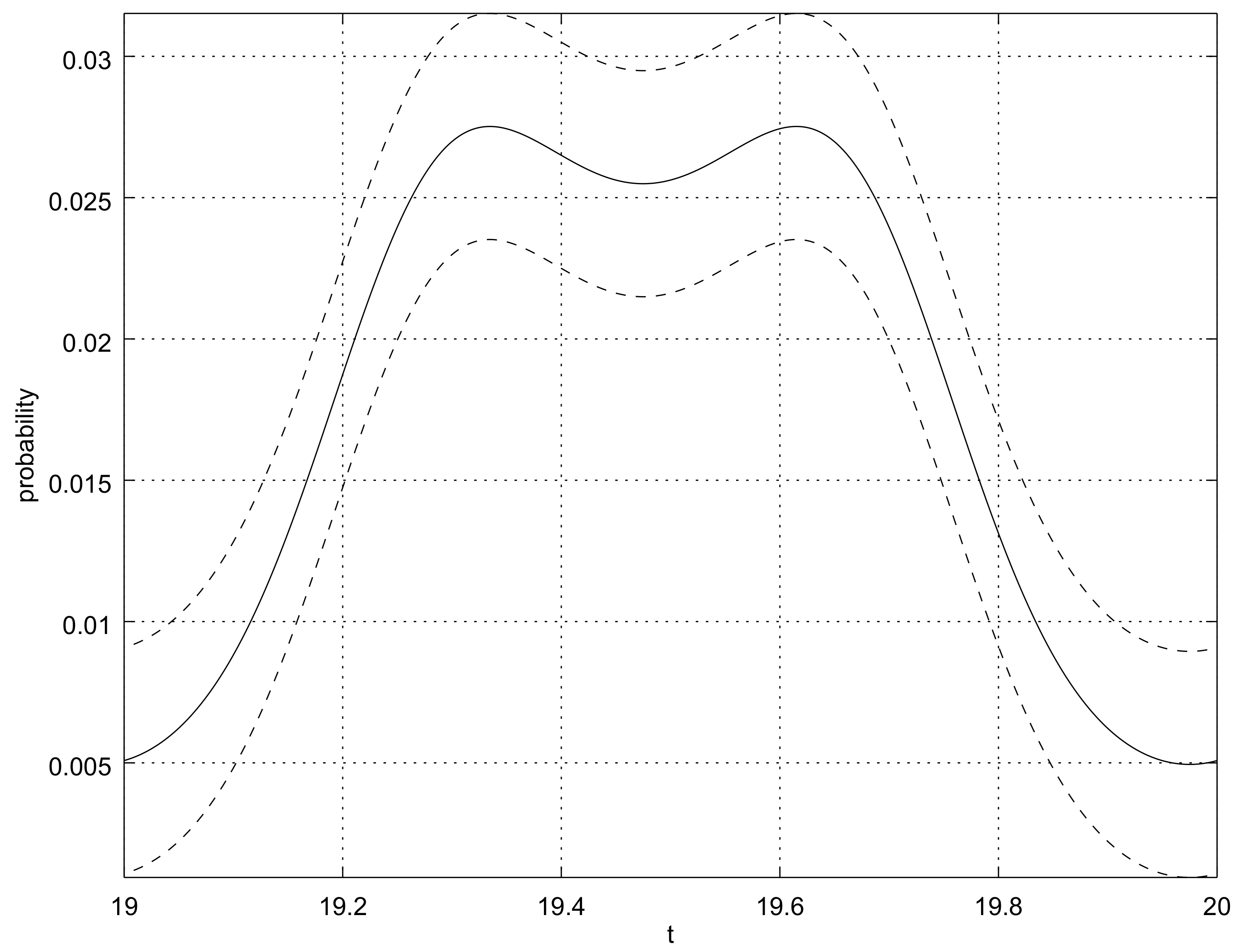
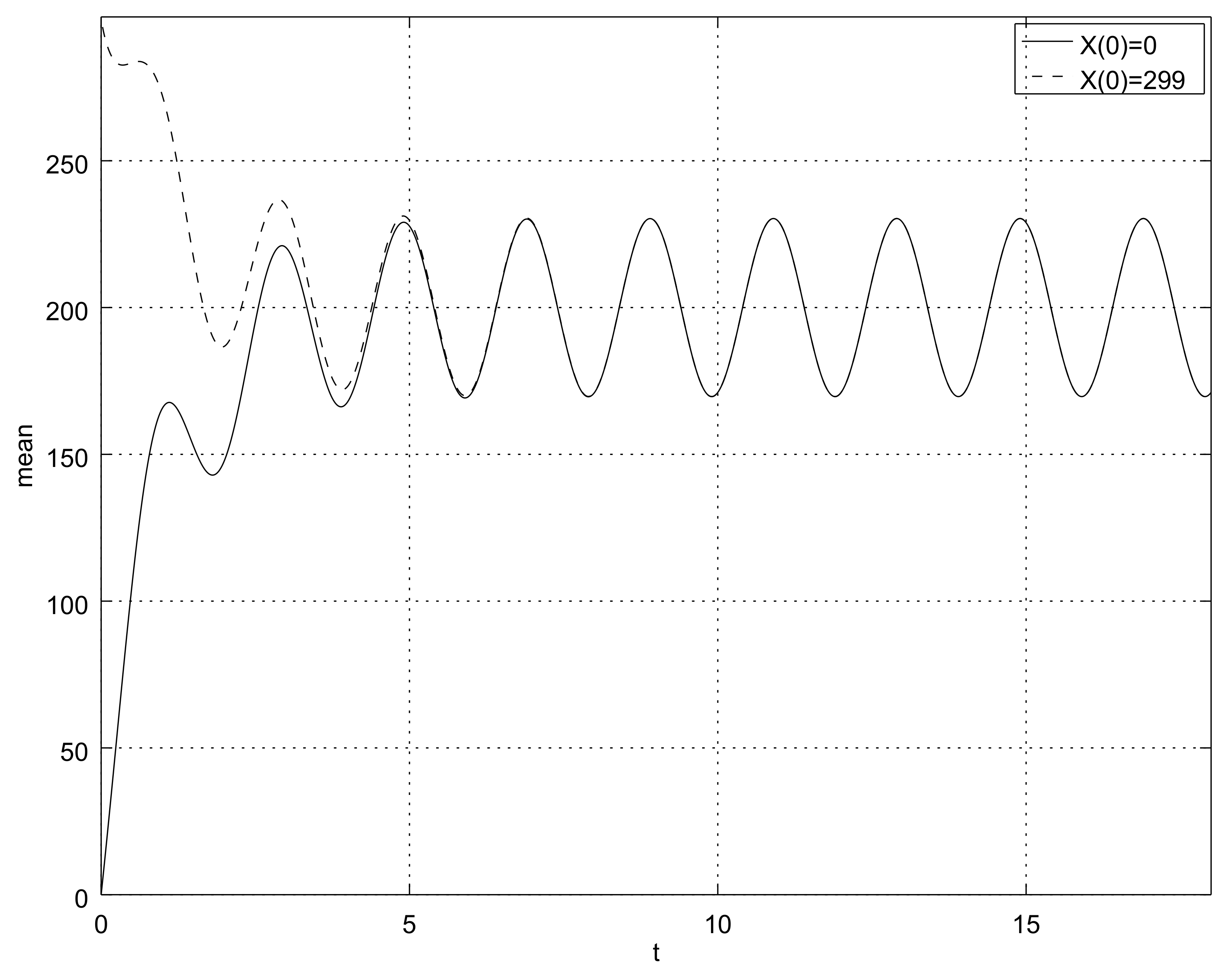
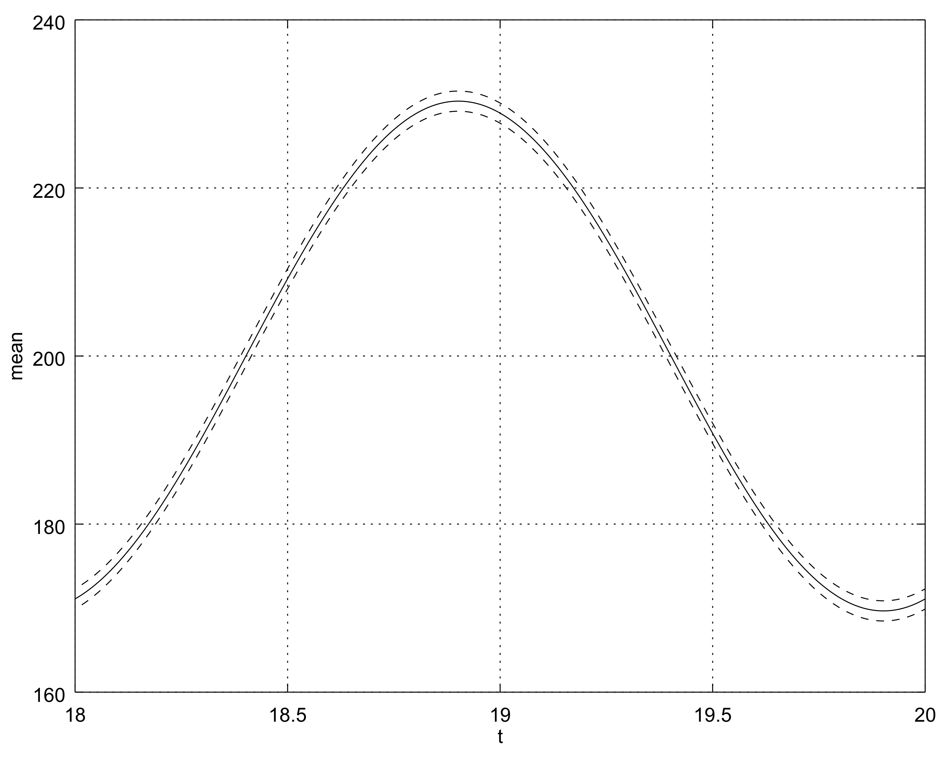
For example, let $\lambda \left(t\right)=1+sin2\pi t$, $\mu \left(t\right)=3$, and $\delta =2$. Therefore, we have

$$\alpha \left(t\right)=\mu -2.5\lambda \left(t\right),{\alpha }^{*}=0.5,W=1.$$

(71)

Furthermore, we follow the method described in [71,72] in detail. Namely, we choose the dimensionality of the truncated process (300 in our case), the interval on which the desired accuracy is achieved ($[0,100]$) in the example under consideration) and the limit interval itself (here it is $[100,101]$).

Figure 8, Figure 9, Figure 10, Figure 11, Figure 12 and Figure 13 expose the plots of the expected number of customers in the system and some of the most probable states.