Article

A General Inertial Viscosity Type Method for Nonexpansive Mappings and Its Applications in Signal Processing

1
Institute of Fundamental and Frontier Sciences, University of Electronic Science and Technology of China, Chengdu 611731, China
2
College of Science, Shijiazhuang University, Shijiazhuang 050035, China
*
Author to whom correspondence should be addressed.
Mathematics 2020, 8(2), 288; https://doi.org/10.3390/math8020288
Submission received: 9 January 2020 / Revised: 6 February 2020 / Accepted: 7 February 2020 / Published: 20 February 2020
(This article belongs to the Special Issue Applied Functional Analysis and Its Applications)

Abstract

:
In this paper, we propose viscosity algorithms with two different inertia parameters for solving fixed points of nonexpansive and strictly pseudocontractive mappings. Strong convergence theorems are obtained in Hilbert spaces and the applications to the signal processing are considered. Moreover, some numerical experiments of proposed algorithms and comparisons with existing algorithms are given to the demonstration of the efficiency of the proposed algorithms. The numerical results show that our algorithms are superior to some related algorithms.

1. Introduction

In this paper, H denotes real Hilbert spaces with inner product · , · and norm · . We denote the set of fixed points of an operator T by Fix ( T ) , more precisely, Fix ( T ) : = { x H : T x = x } .
Recall that a mapping T : H H is said to be an η -strict pseudo-contraction if T x T y 2 η ( I T ) x ( I T ) y 2 x y 2 , x , y H , where η [ 0 , 1 ) is a real number. A mapping T : H H is said to be nonexpansive if T x T y x y , x , y H . It is evident that the class of η -strict pseudo-contractions includes the class of nonexpansive mappings, as T is nonexpansive if and only if T is 0-strict pseudo-contractive. Many classical mathematical problems can be casted into the fixed-point problem of nonexpansive mappings, such as, inclusion problem, equilibrium problem, variational inequality problem, saddle point problem, and split feasibility problem, see [1,2,3]. Approximating fixed points of nonexpansive mappings is an important field in many areas of pure and applied mathematics. One of the most well-known algorithms for solving such a problem is the Mann iterative algorithm [4]:
x n + 1 = ( 1 θ n ) T x n + θ n x n ,
where θ n is a sequence in ( 0 , 1 ) . One knows that the iterative sequence { x n } converges weakly to a fixed point of T provided that n = 0 θ n ( 1 θ n ) = + . This algorithm is slow in terms of convergence speed. Moreover, this algorithm converges is weak. To obtain more effective methods, many authors have done a lot of works in this area, see [5,6,7,8]. A mapping f : H H is called a contraction if there exists a constant in [ 0 , 1 ) such that f ( x ) f ( y ) τ x y , x , y H . One of celebrated ways to study nonexpansive operators is to use a contractive operator, which is a convex combination of the previous contractive operator and the nonexpansive operator. The viscosity type method for nonexpansive mappings is defined as follows,
x n + 1 = ( 1 α n ) T x n + α n f ( x n ) ,
where α n is a sequence in ( 0 , 1 ) , T is the nonexpansive operator, and f is the contractive operator. In this method, a special fixed point of the nonexpansive operator is obtained by regularizing the nonexpansive operator via the contraction. This method was proposed by Attouch [9] in 1996 and further promoted by Moudafi [10] in 2000. Motivated by Moudafi, Takahashi and Takahashi [11] introduced a strong convergence theorem by the viscosity type approximation method for finding the fixed point of nonexpansive mappings in Hilbert spaces. In 2019, Qin and Yao [12] introduced a viscosity iterative method for solving a split feasibility problem. For viscosity approximation methods, one refers to [13,14]. In practical applications, one not only studies different algorithms, but also pursues the speed of these algorithms. To obtain faster convergence algorithms, many scholars have given various acceleration techniques, see, e.g., [15,16,17,18,19]. One of the most commonly used methods is the inertial method. In [20], Polyak introduced an inertial extrapolation based on the heavy ball method for solving the smooth convex minimization problem. Shehu et al. [21] introduced a Halpern-type algorithm with inertial terms for approximating fixed points of a nonexpansive mapping. They obtained strong convergence in real Hilbert spaces under some assumptions on the sequence of parameters. To get a more general inertial Mann algorithm for nonexpansive mappings, Dong et al. [22] introduced a general inertial Mann algorithm which includes some classical algorithms as its special cases; however, they only got the weak convergence results.
Inspired by the above works, we give two algorithms for solving fixed point problems of nonexpansive mappings via viscosity and inertial techniques in this paper. One highlight is that our algorithms, which are more consistent and efficient, are accelerated via the inertial technique and the viscosity technique. In addition, the solution also uniquely solves a monotone variational inequality. Another highlight is that we consider two different inertial parameter sequences comparing with the existing results. We establish strong convergence results in infinite dimensional Hilbert spaces without compactness. We also investigate the applications of the two proposed algorithms to variational inequality problems and inclusion problems. Furthermore, we give some numerical experiments to illustrate the convergence efficiency of our algorithms. The proposed numerical experiments show that our algorithms are superior to some related algorithms.
In this paper, Section 2 is devoted to some required prior knowledge, which will be used in this paper. In Section 3, based on viscosity type method, we propose an algorithm for solving fixed point problems of nonexpansive mappings and give an algorithm for strict pseudo-contractive mappings. In Section 4, some applications of our algorithms in real Hilbert spaces are given. Finally, some numerical experiments of our algorithms and its comparisons with other algorithms in signal processing are given in Section 5. Section 6, the last section, is the final conclusion.

2. Toolbox

In this section, we give some essential lemmas for our main convergence theorems.
Lemma 1
([23]). Let { a n } be a non-negative real sequence and { b n } a real sequence and { α n } a real sequence in ( 0 , 1 ) such that n = 1 α n = . Assume that a n + 1 α n b n + a n ( 1 α n ) , n 1 . If, for every subsequence { a n k } of { a n } satisfying lim inf k ( a n k + 1 a n k ) 0 , lim sup k b n k 0 holds, then lim n a n = 0 .
Lemma 2
([24]).Suppose that T : H H is a nonexpansive mapping. Let { x n } be a vector sequence in H and let p be a vector in H. If x n p and x n T x n 0 . Then p Fix ( T ) .
Lemma 3
([14]). Let { σ n } be a non-negative real sequence such that there exists a subsequence { σ n i } of { σ n } satisfying σ n i < σ n i + 1 for all i N . Then, there exists a nondecreasing sequence { m k } of N such that lim k m k = and the following properties are satisfied for all (sufficiently large) number k N : σ m k σ m k + 1 and σ k σ m k + 1 .
It is known that m k is the largest number in the set { 1 , 2 , , k } such that σ m k < σ m k + 1 .
Lemma 4
([25]). Let { s n } be a sequence of non-negative real numbers such that s n + 1 = ( 1 β n ) s n + δ n , 0 , where { β n } is a sequence in ( 0 , 1 ) with n = 0 β n = and { δ n } satisfies lim sup n δ n β n 0 or n = 0 | δ n | < . Then, lim n s n = 0 .

3. Main Results

In this section, we give two strong convergence theorems for approximating the fixed points of nonexpansive mappings and strict pseudo-contractive mappings. First, we propose some assumptions which will be used in our statements.
Condition 1.
Suppose that { α n } , { β n } and { γ n } are three real sequences in ( 0 , 1 ) satisfying the following conditions.
(1) 
n = 1 α n = and lim n α n = 0 ;
(2) 
lim n θ n α n x n x n 1 = lim n ϵ n α n x n x n 1 = 0 ;
(3) 
α n + β n + γ n = 1 and lim inf n γ n β n > 0 ;
Remark 1.
(1) 
If θ n = ϵ n = 0 , i.e., x n = y n = z n , Algorithm 1 is the classical viscosity type algorithm without the inertial technique.
(2) 
Algorithm 1 is a generalization of Shehu et al. [21]. If f ( x ) = u and θ n = ϵ n , i.e., y n = z n , then it becomes the Shehu et al. Algorithm 1 with e n = 0 .
Algorithm 1 The viscosity type algorithm for nonexpansive mappings
  • Initialization: Let x 0 , x 1 H be arbitrary.
  • Iterative Steps: Given the current iterator x n , calculate x n + 1 as follows:
  • Step 1. Compute
    y n = θ n ( x n x n 1 ) + x n , z n = ϵ n ( x n x n 1 ) + x n .
  • Step 2. Compute
    x n + 1 = α n f ( x n ) + β n y n + γ n T z n .
  • Step 3. Set n n + 1 and go to Step 1.
Remark 2.
The (2) of Condition 1 is well defined, as the inertial parameters θ n and ϵ n in (3) can be chosen such that 0 θ n θ n and 0 ϵ n ϵ n , where
θ n = min θ , δ n x n x n 1 , x n x n 1 , θ , o t h e r w i s e , ϵ n = min ϵ , δ n x n x n 1 , x n x n 1 , ϵ , o t h e r w i s e ,
and { δ n } is a positive sequence such that lim n δ n α n = 0 . It is easy to verify that lim n θ n x n x n 1 = 0 and lim n θ n α n x n x n 1 = 0 .
Theorem 1.
Let T : H H be a nonexpansive mapping with Fix ( T ) and let f : H H be a contraction with constant k [ 0 , 1 ) . Suppose that { x n } is any sequence generated by Algorithm 1 and Condition 1 holds. Then, { x n } converges strongly to p = P Fix ( T ) f ( p ) .
Proof. 
The proof is divided into three steps.
Step 1. One claims that { x n } is bounded.
Let p Fix ( T ) . As y n = θ n ( x n x n 1 ) + x n , one concludes
y n p θ n x n x n 1 + x n p .
Similarly, one gets
z n p x n p + ϵ n x n x n 1 .
From (3), one obtains
x n + 1 p γ n p T z n + β n p y n + α n p f ( x n ) γ n p z n + β n p y n + α n f ( x n ) f ( p ) + f ( p ) p ( 1 α n ( 1 k ) ) x n p   + α n ( 1 k ) ( f ( p ) p + β n θ n α n x n x n 1 + γ n ϵ n α n x n x n 1 1 k ) .
In view of Condition 1 (2), one sees that sup n 1 θ n α n x n x n 1 and sup n 1 ϵ n α n x n x n 1 exist. Taking M : = 3 max f ( p ) p , sup n 1 θ n α n x n x n 1 , sup n 1 ϵ n α n x n x n 1 , one gets from (7) that
x n + 1 p ( 1 α n ( 1 k ) ) x n p + α n ( 1 k ) M max { x n p , M } max { x 1 p , M } .
This implies that { x n } is bounded.
Step 2. One claims that if { x n } converges weakly to z H , then z Fix ( T ) . Letting w n + 1 = α n f ( w n ) + β n w n + γ n T w n , from (1), one arrives at
w n y n θ n | x n x n 1 + w n x n
and
w n z n ϵ n | x n x n 1 + w n x n .
By the definition of w n + 1 , (8) and (9), one obtains
w n + 1 x n + 1 α n f ( w n ) f ( x n ) + β n w n y n + γ n T w n T z n k α n w n x n + β n w n y n + γ n w n z n ( 1 α n ( 1 k ) ) w n x n + ( θ n x n x n 1 + ϵ n x n x n 1 ) .
From Condition 1 and Lemma 4, one sees that (10) implies lim n w n + 1 x n + 1 = 0 . Therefore, it follows from Step 1 that { w n } is bounded. By the definition of w n + 1 , one also obtains
w n + 1 p 2 α n ( f ( w n ) f ( p ) ) + β n ( y n p ) + γ n ( T y n p ) 2 + 2 α n f ( p ) p , w n + 1 p α n k 2 w n p 2 + β n w n p 2 + γ n T w n p 2 β n γ n w n T w n 2 + 2 α n f ( p ) p , w n + 1 p = ( 1 α n ( 1 k 2 ) ) w n p 2 + 2 α n f ( p ) p , w n + 1 p β n γ n w n T w n 2 .
Taking s n = w n p 2 , one sees that (11) is equivalent to
s n + 1 ( 1 α n ( 1 k 2 ) ) s n β n γ n w n T w n 2 + 2 α n f ( p ) p , w n + 1 p .
Now, we show z Fix ( T ) by considering two possible cases on sequence { s n } .
Case 1. Suppose that there exists a n 0 N such that s n + 1 s n for all n n 0 . This implies that lim n s n exists. From (12), one has
β n γ n w n T w n 2 ( 1 α n ( 1 k 2 ) ) s n + 2 α n f ( p ) p , w n + 1 p s n + 1 .
As { w n } is bounded, from Condition 1 and (13), one deduces that
lim n β n γ n w n T w n 2 = 0 .
As lim inf n β n γ n > 0 , (14) implies that
lim n w n T w n 2 = 0 .
As x n z and lim n w n + 1 x n + 1 = 0 , one has w n z . By using Lemma 2, one gets z Fix ( T ) .
Case 2. There exists a subsequence { s n j } of such { s n } that s n j < s n j + 1 for all j N . In this case, it follows from Lemma 3 that there is a nondecreasing subsequence { m k } of N such that lim k m k and the following inequalities hold for all k N :
s m k s m k + 1 a n d s k s m k + 1 .
Using a similar argument as Case 1, it is easy to get that lim k T w m k w m k = 0 . It is known that x n z , which implies x m k z . Therefore, z Fix ( T ) .
Step 3. One claims that { x n } converges strongly to p = P Fix ( T ) f ( p ) . From (11), we deduce that
w n + 1 p 2 ( 1 α n ( 1 k 2 ) ) w n p 2 + 2 α n f ( p ) p , w n + 1 p .
In the following, we show that the sequence { w n p } converges strongly to zero. As { w n } is bounded, in view of Condition 1 and Lemma 1, we only need to show that for each subsequence { w n k p } of { w n p } such that lim inf k ( w n k + 1 p w n k p ) 0 , lim sup k f ( p ) p , w n k + 1 p 0 . For this purpose, one assumes that { w n k p } is a subsequence of { w n p } such that lim inf k ( w n k + 1 p w n k p ) 0 . This implies that
lim inf k ( w n k + 1 p 2 w n k p 2 ) = lim inf k ( ( w n k + 1 p w n k p )     × ( w n k + 1 + p + w n k p ) ) 0 .
From the definition of w n , we obtain
w n k + 1 w n k α n k ( f ( w n k ) w n k ) + γ n k ( T w n k w n k ) α n k f ( w n k ) w n k + γ n k T w n k w n k α n k ( k w n k p + f ( p ) w n k ) + γ n k T w n k w n k .
Using the argument of Case 1 and Case 2 in Step 2, there exists a subsequence of { w n k } , still denoted by { w n k } , such that
lim k T w n k w n k = 0 .
By the boundedness of { w n } , one deduces from Condition 1, (19), and (20) that
lim n w n k + 1 w n k = 0 .
As { w n k } is bounded, there exists a subsequence { w n k j } of { w n k } converges weakly to some z H . This implies that    
lim sup k f ( p ) p , w n k p = lim sup j f ( p ) p , w n k j p = f ( p ) p , z p .
From Step 2, one gets z Fix ( T ) . Since p = P Fix ( T ) f ( p ) , one arrives at
lim sup k f ( p ) p , w n k p = f ( p ) p , z p 0 .
From (21), one obtains
lim sup k f ( p ) p , w n k + 1 p = lim sup k f ( p ) p , w n k p + lim sup k f ( p ) p , w n k + 1 w n k = f ( p ) p , z p 0 .
Therefore, one has w n p 0 . Since lim n w n x n = 0 , one gets x n p 0 . □
In the following, we give a strong convergent theorem for strict pseudo-contractions.
Theorem 2.
Let T : H H be a η-strict pseudo-contraction with Fix ( T ) and let f : H H be a contraction with constant k [ 0 , 1 ) . Suppose that { x n } is a vector sequence generated by Algorithm 2 and Condition 1 holds. Then, { x n } converges strongly to p = P Fix ( T ) f ( p ) .
Algorithm 2 The viscosity type algorithm for strict pseudo-contractions
  • Initialization: Let x 0 , x 1 H be arbitrary and let δ [ η , 1 ) .
  • Iterative Steps: Given the current iterator x n , calculate x n + 1 as follows.
  • Step 1. Compute
    y n = θ n ( x n x n 1 ) + x n , z n = ϵ n ( x n x n 1 ) + x n .
  • Step 2. Compute
    x n + 1 = α n f ( x n ) + β n y n + γ n ( δ z n + ( 1 δ ) T z n ) .
  • Step 3. Set n n + 1 and go to Step 1.
Proof. 
Define Q : H H by Q x = δ x + ( 1 δ ) T x . It is easy to verify that Fix ( T ) = Fix ( Q ) . By the definition of strict pseudo-contraction, one has
Q x Q y 2 = δ x y + ( 1 δ ) T x T y 2 δ ( 1 δ ) ( x y ) ( T x T y ) 2 = δ x y + ( 1 δ ) x y 2 + η ( 1 δ ) ( x y ) ( T x T y ) 2     δ ( 1 δ ) ( x y ) ( T x T y ) 2 x y 2 ( δ η ) ( 1 δ ) ( x y ) ( T x T y ) 2 x y 2 .
Therefore, Q is nonexpansive. Then, we get the conclusions from Theorem 1 immediately. □
In the following, we give some corollaries for Theorem 1.
Recall that T is called a ρ -averaged mapping if and only if it can be written as the average of the identity mapping I and a nonexpansive mapping, that is, T : = ( 1 ρ ) I + ρ S , where ρ ( 0 , 1 ) and S : H H is a nonexpansive mapping. It is known that every ρ -averaged mapping is nonexpansive and Fix ( T ) = Fix ( S ) . A mapping T : H H is said to be quasi-nonexpansive if, for all p Fix ( T ) , T x T p x p , x H . T is said to be strongly nonexpansive if x n y n ( T x n T y n ) 0 , whenever { x n } and { y n } are two sequences in H such that { x n y n } is bounded and x n y n T x n T y n 0 . T is said to be strongly quasi-nonexpansive if T is quasi-nonexpansive and x n T x n 0 whenever { x n } is a bounded sequence in H such that x n p T x n T p 0 for all p Fix ( T ) . By using Theorem 1, we obtain the following corollaries easily.
Corollary 1.
Let H be a Hilbert space and let f : H H be a contraction with constant k [ 0 , 1 ) . Let T : H H be a ρ-average mapping with Fix ( T ) . Suppose that Conditions 1 holds. Then, the sequence { x n } generated by Algorithm 1 converges to p = P Fix ( T ) f ( p ) in norm.
Corollary 2.
Let H be a Hilbert space and let f : H H be a contraction with constant k [ 0 , 1 ) . Let T : H H be a quasi-nonexpansive mapping with Fix ( T ) and I T be demiclosed at the origin. Suppose that Conditions 1 holds. Then, the sequence { x n } generated by Algorithm 1 converges to p = P Fix ( T ) f ( p ) in norm.
Corollary 3.
Let H be a Hilbert space and let f : H H be a contraction with constant k [ 0 , 1 ) . Let T : H H be a strongly quasi-nonexpansive mapping with Fix ( T ) and I T be demiclosed at the origin. Suppose that Conditions 1 holds. Then, the sequence { x n } generated by Algorithm 1 converges to p = P Fix ( T ) f ( p ) in norm.

4. Applications

In this section, we will give some applications of our algorithms to variational equality problems, inclusion problems and corresponding convex minimization problems.

4.1. Variational Inequality Problems

In this subsection, we consider the following variational inequality problem (for short, VIP): find x C such that
A x , y x 0 , y C ,
where A : H H is a single-valued operator and C is a nonempty convex closed set in H. The solutions of VIP 25 is denoted by Ω . It is known that x is a solution of VIP (25) if and only if x = P C ( x λ A x ) , where λ is an arbitrary positive constant. In recent decades, the VIP has received a lot of attention. In order to solve the VIP, various methods have been proposed, see, e.g., [26,27,28]. In this subsection, we will give some applications of our algorithms to the VIP (25). For this purpose, we introduce a lemma proposed by Shehu et al. [21].
Lemma 5.
Let H be a Hilbert space and let C be a nonempty convex and closed set in H. Suppose that A : H H is a monotone L-Lipschitz operator on C and that λ is a positive number. Let V : = P C ( I λ A ) and let S : = V λ ( A V A ) . Then, I V is demi-closed at the origin. Moreover, if λ L < 1 , S is a strongly quasi-nonexpansive operator and Fix ( S ) = Fix ( V ) = Ω .
By using Lemma 5 and Corollary 3, we obtain the following corollary for VIP (25) immediately.
Corollary 4.
Let H be a Hilbert space and let C be a nonempty convex closed set in H. Let f : H H be a contraction with constant k [ 0 , 1 ) . Let A : H H be a monotone L-Lipschitz operator and let τ 0 , 1 L . Suppose that Conditions 1 holds. Then, the sequence { x n } generated by Algorithm 3 converges to p = P Ω f ( p ) in norm.
Proof. 
Let S : = P C ( I τ A ) τ ( A ( P C ( I τ A ) ) A ) . We see from Lemma 5 that S is strongly quasi-nonexpansive and Fix ( S ) = Ω . Then, we get the conclusions from Corollary 3 immediately. □
Algorithm 3 The viscosity type algorithm for solving variational inequality problems
  • Iterative Steps: Given the current iterator x n , calculate x n + 1 as follows.
  • Step 1. Compute
    y n = x n + θ n ( x n x n 1 ) , z n = x n + ϵ n ( x n x n 1 ) .
  • Step 2. Compute
    w n = P C ( I λ A ) z n , x n + 1 = α n f ( x n ) + β n y n + γ n w n λ A w n A z n .
  • Step 3. Set n n + 1 and go to Step 1.

4.2. Inclusion Problems

Let H denote the Hilbert spaces and let A : H H be a single-valued mapping. Then, A is said to be monotone if A x A y , x y 0 , x , y H ; A is said to be α -inverse strongly monotone if A x A y , x y α A ( x ) A ( y ) 2 , x , y H . A set-valued operator A : H 2 H is said to be monotone if x y , u v 0 , x , y H , where u A x and v A y . Furthermore, A said to be maximal monotone if, for all ( y , v ) G r a p h ( A ) and each ( x , u ) H × H , x y , u v 0 implies that u A x . Recall that the resolvent operator J r A : H H associated operator A is defined by J r A = ( I + r A ) 1 x , where r > 0 and I denotes the identity operator on H. If A is a maximal monotone mapping, J r A is a single-valued and firmly nonexpansive mapping. Consider the following simple inclusion problem: find x H such that
0 A x ,
where A : H H is a maximal monotone operator. It is know that 0 A ( x ) if and only if x Fix ( J r A ) . By using Theorem 1, we obtain the following corollary.
Corollary 5.
Let H be a Hilbert space and let f : H H be a contraction with constant k [ 0 , 1 ) . Let A : H H be a maximal monotone operator such that A 1 ( 0 ) . Suppose that Conditions 1 holds. Then, the sequence { x n } generated by Algorithm 4 converges strongly to p = P A 1 ( 0 ) f ( p ) .
Algorithm 4 The viscosity type algorithm for solving inclusion problem (28)
  • Initialization: Let x 0 , x 1 H be arbitrary.
  • Iterative Steps: Given the current iterator x n , calculate x n + 1 as follows.
  • Step 1. Compute
    y n = x n + θ n ( x n x n 1 ) , z n = x n + ϵ n ( x n x n 1 ) .
  • Step 2. Compute
    x n + 1 = α n f ( x n ) + β n y n + γ n J r A ( z n ) .
  • Step 3. Set n n + 1 and go to Step 1.
Proof. 
As Fix ( J r A ) = A 1 ( 0 ) and J r A is firmly nonexpansive, one has that J r A is 1 2 -averaged. Therefore, there exists a nonexpansive mapping S such that J r A = 1 2 I + 1 2 S and Fix ( J r A ) = Fix ( S ) . By using Corollary 1, we obtain the conclusions immediately. □
Now, we solve the following convex minimization problem.
min x H h ( x ) ,
where h : H ( , + ] is a proper lower semi-continuous closed convex function. The subdifferential operator h ( x ) of h ( x ) is defined by h ( x ) = { u H : h ( y ) h ( x ) + u , y x , y H } . It is known that h ( x ) is maximal monotone, and x is a solution of problem (31) if and only if 0 h ( x ) . Taking A = h ( x ) , we have J r A = p r o x r h , where r > 0 and p r o x r h is defined by
prox r h ( u ) = arg min x H 1 2 r x u 2 + h ( x ) .
Corollary 6.
Let H be a Hilbert space and let f : H H be a contraction with constant k [ 0 , 1 ) . Let h : H ( , + ] be a proper closed lower semi-continuous convex function such that arg min h . Suppose that Conditions 1 holds. Then, the sequence { x n } generated by Algorithm 5 converges to a solution of convex minimization problem (31) in norm.
Algorithm 5 The viscosity type algorithm for solving convex minimization problems
  • Initialization: Let x 0 , x 1 H be arbitrary.
  • Iterative Steps: Given the current iterator x n , calculate x n + 1 as follows.
  • Step 1. Compute
    y n = x n + θ n ( x n x n 1 ) , z n = x n + ϵ n ( x n x n 1 ) .
  • Step 2. Compute
    x n + 1 = α n f ( x n ) + β n y n + γ n p r o x r h ( z n ) .
  • Step 3. Set n n + 1 and go to Step 1.
Proof. 
It is known that the subdifferential operator h is maximal monotone since h is a proper, closed lower semi-continuous, convex function. Therefore, prox r h = J r h . Then, we get the conclusions from Corollary 5 immediately. □
In the following, we consider the following inclusion problem: find x H such that
0 A ( x ) + B ( x ) ,
where A : H H be an α -inverse strongly monotone mapping and let B : H 2 H be a set-valued maximal monotone operator. It is known that Fix ( J r B ( I r A ) ) = ( A + B ) 1 ( 0 ) . Many problems can be modelled as the inclusion problem, such as, convex programming problems, inverse problems, split feasibility problems, and minimization problems, see [29,30,31,32]. Moreover, this problem is also widely applied in machine learning, signal processing, statistical regression, and image restoration, see [33,34,35]. By using Theorem 1, we obtain the following corollary.
Corollary 7.
Let H be a Hilbert space and let f : H H be a contraction with constant k [ 0 , 1 ) . Let A : H H be a α-inverse strongly monotone mapping with 0 < r = 2 α and let B : H 2 H be a maximal monotone operator. Suppose that ( A + B ) 1 ( 0 ) and Conditions 1 holds. Then, the sequence { x n } generated by Algorithm 3 converges to p = P ( A + B ) 1 ( 0 ) f ( p ) in norm.
Proof. 
As A is inverse strongly monotone, one has that ( I r A ) is nonexpansive. Therefore, the operator J r B ( I r A ) is nonexpansive. Then, we get the conclusions from Theorem 1 immediately. □

5. Numerical Results

In this section, we give three numerical examples to illustrate the computational performance of our proposed algorithms. All the programs are performed in MATLAB2018a on a PC Desktop Intel(R) Core(TM) i5-8250U CPU @ 1.60 GHz 1.800 GHz, RAM 8.00 GB.
Example 1.
In this example, we consider the following case that the usual gradient method is not convergent. Take the feasible set as C : = { 5 x i 5 , i = 1 , 2 , , m } and an m × m square matrix A : = a i j 1 i , j m whose terms are given by
a i j = 1 , i f j = m + 1 i a n d j < i , 1 , i f j = m + 1 i a n d j > i , 0 , o t h e r w i s e .
One knows that zero vector x = ( 0 , , 0 ) is a solution of this problem. First, one tests the Algorithm 3 with different choices of inertial parameter θ n and ϵ n . Setting f ( x ) = 0.5 x , δ n = 1 ( n + 1 ) 2 , α n = n ( n + 1 ) 1.1 , β n = γ n = 1 α n 2 , λ = 0.7 , the numerical results are shown in Table 1 and Table 2.
To compare the efficiency between algorithms, we consider our proposed Algorithm 3, the extragradient method (EGM) in [36], the subgradient extragradient method (SEGM) in [26], and the new inertial subgradient extragradient method (NISEGM) in [27]. The parameters are selected as follows. The initial points x 0 , x 1 R m are generated randomly in MATLAB and we take different values of m into consideration. In EGM, SEGM, we take λ = 0.7 . In Algorithm 3, we take f ( x ) = 0.5 x , λ = 0.7 , δ n = 1 ( n + 1 ) 2 , θ = 0.7 and ϵ = 0.8 in (4), α n = n ( n + 1 ) 1.1 , β n = γ n = 1 α n 2 . We set α n = 0.1 , τ n = n ( n + 1 ) 1.1 , λ n = 0.8 in NISEGM. The stopping criterion is E n = x n x 2 < 10 4 . The results are proposed in Table 3 and Figure 1.
Remark 3.
By Table 1 and Table 2, one concludes that the number of the iteration is small for the Algorithm 3 with θ [ 0.5 , 1 ] and ϵ [ 0.5 , 1 ] .
Remark 4.
(1)
By numerical results of Example 1, we find that our Algorithm 3 is efficient, easy to implement and fast. Moreover, dimensions do not affect the computational performance of our algorithm.
(2)
Obviously, by Example 1, we also find that our proposed Algorithm 3 outperforms the extragradient method (EGM), the subgradient extragradient method (SEGM) and the new inertial subgradient extragradient method (NISEGM) in both CPU time and number of iterations.
Algorithm 6 The viscosity type algorithm for solving inclusion problem (34)
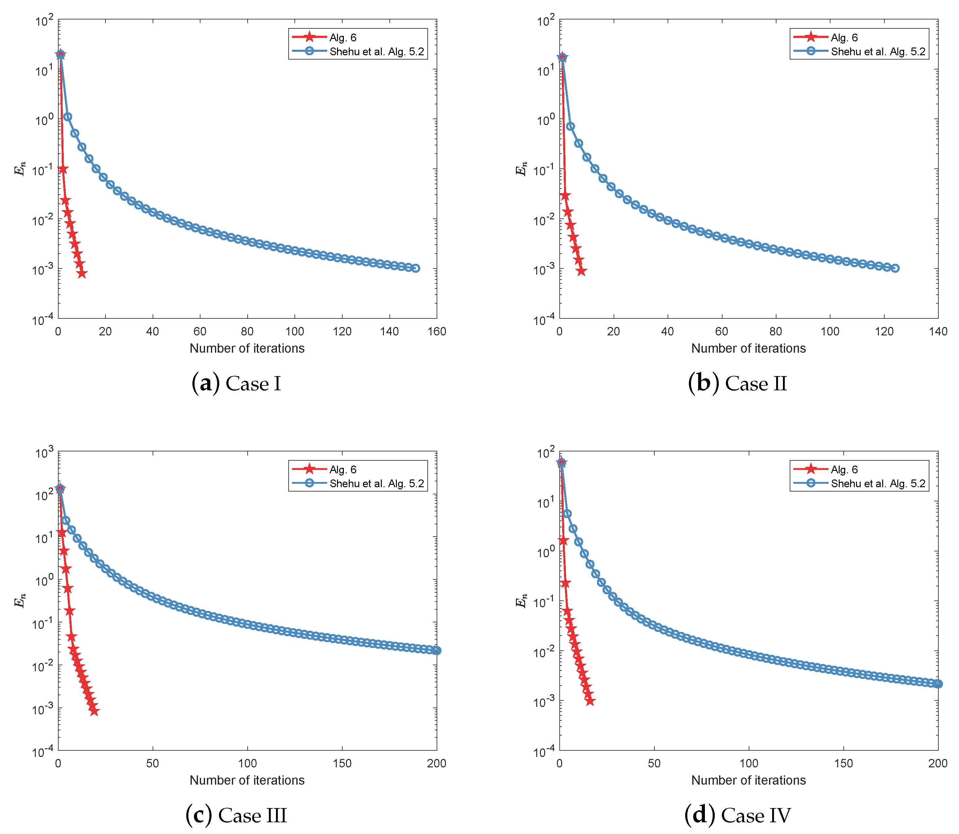
  • Initialization: Let x 0 , x 1 H be arbitrary.
  • Iterative Steps: Given the current iterator x n , calculate x n + 1 as follows:
  • Step 1. Compute
    y n = x n + θ n ( x n x n 1 ) , z n = x n + ϵ n ( x n x n 1 ) .
  • Step 2. Compute
    x n + 1 = α n f ( x n ) + β n y n + γ n J r B ( I r A ) z n .
  • Step 3. Set n n + 1 and go to Step 1.
Example 2.
In this example, we consider H = L 2 ( [ 0 , 2 π ] ) and the following half-space,
C = x L 2 ( [ 0 , 2 π ] ) | 0 2 π x ( t ) d t 1 , a n d Q = x L 2 ( [ 0 , 2 π ] ) | 0 2 π x ( t ) sin ( t ) 2 d t 16 .
Define a linear continuous operator T : L 2 ( [ 0 , 2 π ] ) L 2 ( [ 0 , 2 π ] ) , where ( T x ) ( t ) : = x ( t ) . Then T x ( t ) = x ( t ) and T = 1 . Now, we solve the following problem,
f i n d x C s u c h t h a t T x Q .
As ( T x ) ( t ) = x ( t ) , (37) is actually a convex feasibility problem: find x C Q . Moreover, it is evident that x ( t ) = 0 is a solution. Therefore, the solution set of (37) is nonempty. Take A x = 1 2 T x P Q T x 2 = T I P Q T x and B = i C . Then (37) can be written in the form (34). It is clear that A is 1-Lipschitz continuous and B is maximal monotone. For our numerical computation, we can also write the projections onto set C and the projections onto set Q as follows, see [37].
P C ( z ) = 1 0 2 π z ( t ) d t 4 π 2 + z , 0 2 π z ( t ) d t > 1 , z , 0 2 π z ( t ) d t 1 .
and
P Q ( w ) = sin + 4 0 2 π | w ( t ) sin ( t ) | 2 d t ( w sin ) , 0 2 π | w ( t ) sin ( t ) | 2 d t > 16 , w , 0 2 π | w ( t ) sin ( t ) | 2 d t 16 .
In this numerical experiment, we consider different initial values x 0 and x 1 . The error of the iterative algorithms is denoted by
E n = 1 2 P C x n x n 2 2 + 1 2 P Q T x n T x n 2 2 .
Now, we give some numerical experiment comparisons between our Algorithm 6 and the Algorithm 5.2 proposed by Shehu et al. [21]. We denote this algorithm by Shehu et al. Algorithm 5.2. In the Shehu et al. Algorithm 5.2, one sets λ = 0.25 , ϵ n = 1 ( n + 1 ) 2 , θ = 0.5 , α n = 1 n + 1 , β n = γ n = n 2 ( n + 1 ) , e n = 1 ( n + 1 ) 2 . In Algorithm 6, one sets f ( x ) = 0.5 x , r = 0.25 , δ n = 1 ( n + 1 ) 2 , θ = 0.5 , ϵ = 0.7 , α n = 1 n + 1 , and β n = γ n = n 2 ( n + 1 ) . Our stopping criterion is maximum iteration 200 or E n < 10 3 . The results are proposed in Table 4 and Figure 2.
Remark 5.
(1)
Also, by observing numerical results of Example 2, we find that our Algorithm 6 is more efficient and faster than the Shehu et al.’s Algorithm 5.2.
(2)
Our Algorithm 6 is consistent since the choice of initial value does not affect the number of iterations needed to achieve the expected results.
Example 3.
In this example, we consider a linear inverse problem: b = A x 0 + w , where x 0 R N is the (unknown) signal to recover, w R M is a noise vector, and A R M × N models the acquisition device. To recover an approximation of the signal x 0 , we use the Basis Pursuit denoising method. That is, one uses the 1 norm as a sparsity enforcing penalty.
min x R N Φ ( x ) = 1 2 b A x 2 + λ x 1 ,
where x 1 = i x i and λ is a parameter that is relate to noise w. It is known that (38) is referred as the least absolute selection and shrinkage operator problem, that is, the LASSO problem. The LASSO problem (38) is a special case of minimizing F + G , where
F ( x ) = 1 2 b A x 2 , a n d G ( x ) = λ x 1 .
It is easy to see that F is a smooth function with L-Lipschitz continuous gradient F ( x ) = A ( A x b ) , where L = A A . The 1 -norm is “simple", as its proximal operator is a soft thresholding:
prox γ G ( x k ) = max 0 , 1 λ γ x k x k .
In our experiment, we want to recover a sparse signal x 0 R N with k ( k N ) non-zero elements. A simple linearized model of signal processing is to consider a linear operator, that is, a filtering A x = φ 🟉 x , where φ is a second derivative of Gaussian. We wish to solve b = A x 0 + w , where w is a realization of Gaussian white noise with variance 10 2 . Therefore, we need to solve the (38). We compare our Algorithm 6 with another strong convergence algorithm, which was proposed by Gibali and Thong in [38]. We denote this algorithm by G-T Algorithm 1. In addition, we also compare the algorithms with the classic Forward–Backward algorithm in [33]. Our parameter settings are as follows. In all algorithms, we set regularization parameter λ = 1 2 in (38). In the Forward–Backward algorithm, we set step size γ = 1.9 / L . In G-T Algorithm 1, we set step size γ = 1.9 / L , α n = 1 n + 1 , β n = n 2 ( n + 1 ) and μ = 0.5 . In Algorithm 6, we set step size r = 1.9 / L , f ( x ) = 0.1 x , θ = ϵ = 0.9 , δ n = 1 ( n + 1 ) 2 , α n = 1 n + 1 , β n = 1 1000 ( n + 1 ) 3 , γ n = 1 α n β n . We take the maximum number of iterations 5 × 10 4 as a common stopping criterion. In addition, we use the signal-to-noise ratio (SNR) to measure the quality of recovery, and a larger SNR means a better recovery quality. Numerical results are proposed in Table 5 and Figure 3, Figure 4 and Figure 5. We tested the computational performance of the above algorithms in different dimension N and different sparsity k (Case I: N = 400 , k = 12 ; Case II: N = 400 , k = 20 ; Case III: N = 1000 , k = 30 ; Case IV: N = 1000 , k = 50 ). Figure 3 shows the original and noise signals in different dimension N and different sparsity k. Figure 4 shows the recovery results of different algorithms under different situation, the corresponding numerical results are shown in Table 5. Figure 5 shows the convergence behavior of Φ ( x ) in (38) with the number of iterations.
Remark 6.
(1)
The LASSO problem in Example 3 also shows that our proposed algorithm is consistent and more efficient. Furthermore, dimensions and sparsity do not affect the computational performance of our proposed Algorithm 6, see Table 5 and Figure 4 and Figure 5.
(2)
The numerical results also show that our Algorithm 6 is superior than the algorithm proposed by Gibali and Thong [38] in terms of computational performance and accuracy.
(3)
In addition, there is little difference between our Algorithm 6 and the classical Forward–Backward algorithm in computational performance and precision. Note that the Forward–Backward algorithm is weak convergence in the infinite dimensional Hilbert spaces; however, our proposed algorithms is strongly convergent (see Corollary 7 and Example 2).

6. Conclusions

In this paper, we proposed a viscosity algorithm with two different inertia parameters for solving fixed-point problem of nonexpansive mappings. We also established a strong convergence theorem for strict pseudo-contractive mappings. By choosing different parameter values in inertial sequences, we analyzed the convergence behavior of our proposed algorithms. One highlight is that our algorithms are based on two different inertial parameter sequences comparing with the exiting ones. accelerated via the inertial technique and the viscosity technique. Another highlight is that, to show the effectiveness of our algorithms, we compare our algorithms with other existing algorithms in the convergence rate and applications in signal processing. Numerical experiments show that our algorithms are consistent and efficient. Finally, we remark that the framework of the space is a Hilbert space, it is of interest to further our results to the framework of Banach spaces or Hadamard manifolds.

Author Contributions

All the authors contributed equally to this work. All authors have read and agreed to the published version of the manuscript.

Funding

This paper was supported by the National Natural Science Foundation of China under Grant 11601348.

Acknowledgments

The authors are grateful to the referees for useful suggestions, which improved the contents of this paper.

Conflicts of Interest

The authors declare no conflicts of interest.

References

  1. Chidume, C.E.; Romanus, O.M.; Nnyaba, U.V. An iterative algorithm for solving split equilibrium problems and split equality variational inclusions for a class of nonexpansive-type maps. Optimization 2018, 67, 1949–1962. [Google Scholar] [CrossRef]
  2. Cho, S.Y.; Kang, S.M. Approximation of common solutions of variational inequalities via strict pseudocontractions. Acta Math. Sci. 2012, 32, 1607–1618. [Google Scholar] [CrossRef]
  3. Qin, X.; Cho, S.Y.; Yao, J.C. Weak and strong convergence of splitting algorithms in Banach spaces. Optimization 2020, 69, 243–267. [Google Scholar] [CrossRef]
  4. Mann, W.R. Mean value methods in iteration. Proc. Amer. Math. Soc. 1953, 4, 506–510. [Google Scholar] [CrossRef]
  5. Chang, S.S.; Wen, C.F.; Yao, J.C. Zero point problem of accretive operators in Banach spaces. Bull. Malays. Math. Sci. Soc. 2019, 42, 105–118. [Google Scholar] [CrossRef]
  6. Chang, S.S.; Wen, C.F.; Yao, J.C. Common zero point for a finite family of inclusion problems of accretive mappings in Banach spaces. Optimization 2018, 67, 1183–1196. [Google Scholar] [CrossRef]
  7. Cho, S.Y.; Li, W.; Kang, S.M. Convergence analysis of an iterative algorithm for monotone operators. J. Inequal. Appl. 2013, 2013, 199. [Google Scholar] [CrossRef] [Green Version]
  8. Qin, X.; Cho, S.Y.; Wang, L. Strong convergence of an iterative algorithm involving nonlinear mappings of nonexpansive and accretive type. Optimization 2018, 67, 1377–1388. [Google Scholar] [CrossRef]
  9. Attouch, H. Viscosity approximation methods for minimization problems. SIAM J. Optim. 1996, 6, 769–806. [Google Scholar] [CrossRef]
  10. Moudafi, A. Viscosity approximation methods for fixed-points problems. J. Math. Anal. Appl. 2000, 241, 46–55. [Google Scholar] [CrossRef] [Green Version]
  11. Takahashi, S.; Takahashi, W. Viscosity approximation methods for equilibrium problems and fixed point problems in Hilbert spaces. J. Math. Anal. Appl. 2007, 331, 506–515. [Google Scholar] [CrossRef] [Green Version]
  12. Qin, X.; Yao, J.C. A viscosity iterative method for a split feasibility problem. J. Nonlinear Convex Anal. 2019, 20, 1497–1506. [Google Scholar]
  13. Qin, X.; Cho, S.Y.; Wang, L. Iterative algorithms with errors for zero points of m-accretive operators. Fixed Point Theory Appl. 2013, 2013, 148. [Google Scholar] [CrossRef] [Green Version]
  14. Maingé, P.E. A hybrid extragradient-viscosity method for monotone operators and fixed point problems. SIAM J. Optim. 2008, 47, 1499–1515. [Google Scholar] [CrossRef]
  15. Takahashi, W.; Xu, H.K.; Yao, J.C. Iterative methods for generalized split feasibility problems in Hilbert spaces. Set-Valued Var. Anal. 2015, 23, 205–221. [Google Scholar] [CrossRef]
  16. Qin, X.; Cho, S.Y.; Wang, L. A regularization method for treating zero points of the sum of two monotone operators. Fixed Point Theory Appl. 2014, 2014, 75. [Google Scholar] [CrossRef] [Green Version]
  17. Cho, S.Y.; Bin Dehaish, B.A. Weak convergence of a splitting algorithm in Hilbert spaces. J. Appl. Anal. Comput. 2017, 7, 427–438. [Google Scholar]
  18. Qin, X.; Wang, L.; Yao, J.C. Inertial splitting method for maximal monotone mappings. J. Nonlinear Convex Anal. 2020, in press. [Google Scholar]
  19. Qin, X.; Cho, S.Y. Convergence analysis of a monotone projection algorithm in reflexive Banach spaces. Acta Math. Sci. 2017, 37, 488–502. [Google Scholar] [CrossRef]
  20. Polyak, B.T. Some methods of speeding up the convergence of iteration methods. USSR Comput. Math. Math. Phys. 1964, 4, 1–17. [Google Scholar] [CrossRef]
  21. Shehu, Y.; Iyiola, O.S.; Ogbuisi, F.U. Iterative method with inertial terms for nonexpansive mappings: applications to compressed sensing. Numer Algor. 2019. [Google Scholar] [CrossRef]
  22. Dong, Q.L.; Cho, Y.J.; Rassias, T.M. General inertial Mann algorithms and their convergence analysis for nonexpansive mappings. In Applications of Nonlinear Analysis; Rassias, T.M., Ed.; Springer: Berlin, Gernmany, 2018; pp. 175–191. [Google Scholar]
  23. Saejung, S.; Yotkaew, P. Approximation of zeros of inverse strongly monotone operators in Banach spaces. Nonlinear Anal. 2012, 75, 742–750. [Google Scholar] [CrossRef]
  24. Goebel, K.; Kirk, W.A. Topics in Metric Fixed Point Theory; Cambridge University Press: Cambridge, UK, 1990; Volume 28. [Google Scholar]
  25. Xu, H.K. Iterative algorithms for nonlinear operators. J. Lond. Math. Soc. 2002, 66, 240–256. [Google Scholar] [CrossRef]
  26. Censor, Y.; Gibali, A.; Reich, S. Strong convergence of subgradient extragradient methods for the variational inequality problem in Hilbert space. Optim. Methods Softw. 2011, 26, 827–845. [Google Scholar] [CrossRef]
  27. Fan, J.; Liu, L.; Qin, X. A subgradient extragradient algorithm with inertial effects for solving strongly pseudomonotone variational inequalities. Optimization 2019, 1–17. [Google Scholar] [CrossRef]
  28. Malitsky, Y.V.; Semenov, V.V. A hybrid method without extrapolation step for solving variational inequality problems. J. Glob. Optim. 2015, 61, 193–202. [Google Scholar] [CrossRef] [Green Version]
  29. Takahahsi, W.; Yao, J.C. The split common fixed point problem for two finite families of nonlinear mappings in Hilbert spaces. J. Nonlinear Convex Anal. 2019, 20, 173–195. [Google Scholar]
  30. Dehaish, B.A.B. Weak and strong convergence of algorithms for the sum of two accretive operators with applications. J. Nonlinear Convex Anal. 2015, 16, 1321–1336. [Google Scholar]
  31. Qin, X.; Petrusel, A.; Yao, J.C. CQ iterative algorithms for fixed points of nonexpansive mappings and split feasibility problems in Hilbert spaces. J. Nonlinear Convex Anal. 2018, 19, 157–165. [Google Scholar]
  32. Cho, S.Y. Strong convergence analysis of a hybrid algorithm for nonlinear operators in a Banach space. J. Appl. Anal. Comput. 2018, 8, 19–31. [Google Scholar]
  33. Combettes, P.L.; Wajs, V. Signal recovery by proximal forward-backward splitting. Multiscale Model. Simul. 2005, 4, 1168–1200. [Google Scholar] [CrossRef] [Green Version]
  34. An, N.T.; Nam, N.M. Solving k-center problems involving sets based on optimization techniques. J. Glob. Optim. 2020, 76, 189–209. [Google Scholar] [CrossRef]
  35. Qin, X.; An, N.T. Smoothing algorithms for computing the projection onto a Minkowski sum of convex sets. Comput. Optim. Appl. 2019, 74, 821–850. [Google Scholar] [CrossRef] [Green Version]
  36. Korpelevich, G.M. The extragradient method for finding saddle points and other problems. Matecon 1976, 12, 747–756. [Google Scholar]
  37. Bauschke, H.H.; Combettes, P.L. Convex Analysis and Monotone Operator Theory in Hilbert Spaces; Springer: New York, NY, USA, 2011. [Google Scholar]
  38. Gibali, A.; Thong, D.V. Tseng type methods for solving inclusion problems and its applications. Calcolo 2018, 55, 49. [Google Scholar] [CrossRef]
Figure 1. Convergence behavior of iteration error { E n } with different dimension in Example 1.
Mathematics 08 00288 g001
Figure 2. Convergence behavior of iteration error { E n } with different initial values in Example 2.
Mathematics 08 00288 g002
Figure 3. Original signals and noise signals at different N and k in Example 3.
Mathematics 08 00288 g003
Figure 4. Recovery results under different algorithms in Example 3.
Mathematics 08 00288 g004
Figure 5. Convergence behavior of { Φ ( x ) } with different N and k in Example 3.
Mathematics 08 00288 g005
Table 1. Number of iterations of Algorithm 3 with θ = 0.5 , m = 100 .
Initial Value ϵ 00.10.20.30.40.50.60.70.80.91
10 × rand(m,1)Iter.2423232322222221212121
100 × rand(m,1)Iter.2727262626252525252525
1000 × rand(m,1)Iter.3131303030292929292929
Table 2. Number of iterations of Algorithm 3 with ϵ = 0.7 , m = 100 .
Initial Value θ 00.10.20.30.40.50.60.70.80.91
10 × rand(m,1)Iter.2423232222212121212122
100 × rand(m,1)Iter.2727262625252525252525
1000 × rand(m,1)Iter.3030302929292828282828
Table 3. Comparison between Algorithm 3, EGM, SEGM, and NISEGM in Example 1.
Algorithm 3Algorithm EGMAlgorithm SEGMAlgorithm NISEGM
mIter.Time (s)Iter.Time (s)Iter.Time (s)Iter.Time (s)
100240.0102910.0147930.0194840.0121
1000270.0548990.12651010.1376920.1136
2000280.30071010.78521040.7018940.6516
5000291.65821054.28791074.4691974.0239
Table 4. Comparison between our Algorithm 6 and Shehu et al.’s Algorithm 5.2 in Example 2.
Algorithm 6Shehu et al.’s Algorithm 5.2
CasesInitial ValuesIter.Time (s)Iter.Time (s)
I x 0 = t 2 10 x 1 = t 2 10 93.469015145.7379
II x 0 = t 2 10 x 1 = 2 t 16 72.962912438.3933
III x 0 = t 2 10 x 1 = e t / 2 2 187.000220061.6568
IV x 0 = t 2 10 x 1 = 5 sin ( 2 t ) 2 155.842320062.5465
Table 5. Comparison the SNR between Algorithm 6, G-T Algorithm 1, and Forward–Backward in Example 3.
CasesNkG-T Algorithm 1Algorithm 6Forward–Backward
I4001216.242116.374216.3930
II400205.39945.43775.4418
III1000306.74196.77496.7792
IV1000503.24933.25533.2561

