1. Introduction
The capacity [
1], also called fuzzy measure [
2,
3], or nonadditive measure [
4,
5], extends the probability measure’s additivity with respect to disjoint subsets into its nonadditivity (subadditivity, superadditivity, or additivity), which means the capacity only needs to satisfy the monotonicity with respect to set inclusion [
6,
7,
8].
In the capacity based decision making context, the decision preference information can be represented through the values of subsets’ capacity or its equivalent representations such as the simultaneous interaction index [
9,
10], nonadditivity index [
5,
11] and nonmodularity index [
12]. Nonadditivity is an explicit interaction index specially for describing the interaction phenomenon among criteria associated with nonadditivity and meanwhile has some good mathematic properties and intuitive explanations in accordance with decision common sense [
5]. This is also the reason we choose nonadditivity to mainly describe the interaction among criteria in the following.
Besides using the comparison or interval form of the equivalent transformations’ values of criteria subsets, the decision preference can also be represented by the overall evaluations of typical or historical decision alternatives [
13], or by some special types of capacities, like
-capacity [
2],
k-additive capacity [
14],
p-symmetric capacity [
15],
k-maxitive and minitive capacity [
16],
k-interactive capacity [
17], and
k-order upper and lower representative capacity [
18]. Almost all of these three types of decision preference information can be commonly turned into a collection of linear constraints [
3].
Generally speaking, there are two approaches to transform all the decision preferences into the final decision result. One is to adopt a principle to obtain the optimal capacity, and the corresponding nonlinear integral values, like Choquet integral or Sugeno integral values, of decision alternatives are taken as references to make the final decision. These principles include least-squares principle [
13,
19,
20], the least absolute deviation criterion [
21], the maximum split approaches [
20,
22], the maximum entropy principle [
23,
24,
25,
26], the maximum log-likelihood principle [
27,
28,
29], the compromise principle [
30] and the MCCPI (multicriteria correlation preference information) based minimum divergence principle [
31,
32]. However, one can figure out that different principles may lead to different results and every single principle can neither reveal all dominance relationships among alternatives nor the frequencies, probabilities or credibilities of these dominances.
The other approach is to use the random generation of capacity within the feasible region defined by decision preference to simulate the whole dominance relationship among decision alternatives together with the estimated probabilities, and finally get the most confidential decision result. Combarro et al. [
33,
34,
35] proposed the random node and minimum plus based capacity random generation methods, but these methods only consider the boundary and monotonicity conditions (see definition of capacity), without imposing any further preference information constraints. In order to simultaneously consider the complex decision preference constraints, Wu et al. [
36] provided a Choquet integral and linear programming based random generation method as well as the comprehensive decision method. However, this method involves a great many times of linear programming construction and solving. The computation cost is a huge burden for a personal computer when decision criteria number
or the generated capacity number is large; for instance, 5000 capacity with five criteria. So, its applicability is limited in some situations.
In this paper, we propose two types of quasi-random generation methods based on the nonadditivity index which involve no linear programmings and then work with rather efficient execution performance. The method can also flexibly show the relatively complex interaction preference upon decision criteria. We found that, through some empirical tests, the quasi-random generation methods have relatively good performances on statistics characteristic of generated capacities compared with the result by real random generation methods. The decision example further shows that the proposed methods are relatively easier to establish and apply for saving the effort of constructing the optimal model and the objective function and can be taken as competent substitutes for the real random generation based decision making scheme in some situations. In summary, compared to the existing capacity random generation methods, the proposed methods can not only represent additional decision preference about complex interaction phenomena among decision criteria but also have some relative advantages in dealing with large scale decision making problems.
This paper is organized as follows. After the introduction, we present some information about the capacity, nonadditivity index and the Choquet integral in
Section 2. In
Section 3, we briefly summarize the presentation form of the decision preference information and show the Choquet integral based random generation algorithm as well as its comprehensive decision aid algorithm.
Section 4 is devoted to the rationale and process of the nonadditivity index based quasi-random generation algorithms. An empirical analysis of the proposed methods is given in
Section 5. Finally, we conclude the paper in
Section 6.
2. Preliminaries
Let , , be the set of decision criteria, be the power set of N, and be the cardinality of subset .
Definition 1 ([
1,
2]).
A capacity on N is a set function such that (Boundary condition) , ; (Monotonicity condition) , implies . The quantity of
is considered as the importance of
A to the decision problem [
37,
38]. The nonadditivity is one of the explicit properties produced from monotonicity, which can be described through the following definition.
Definition 2 ([
5,
11]).
A capacity μ on N is said to be ★-additive, ifFurthermore, μ is said to be ★-additive within , ifwhere “★-additive” stands for “additive (resp. superadditive, subadditive, strict superadditive, and strict subadditive)”, “” stands for “”. It is a common interpretation that an additive capacity means that the decision criteria are independent; a strict superadditive (respectively strict subadditive, superadditive, and subadditive) capacity indicates that all criteria are mutually complementary (substitutive, nonsubstitutive, and noncomplementary).
Definition 3 ([
5]).
The nonadditivity index of μ is defined as Theorem 1 ([
5]).
If a capacity μ on N is ★-additive, then , , . If a capacity μ on N is ★-additive within , then , , . This means that the nonadditivity index reflects the above common interpretation [
5,
12,
39].
Theorem 2 ([
5]).
, . This means the nonadditivity index has uniform range , then the interaction of subsets with different cardinalities can be directly compared.
Theorem 3 ([
5]).
, , and , where is a capacity on N such that if , , and otherwise; is a capacity on N such that if , and otherwise. One can figure out that and describe two opposite extreme interaction situations between criteria within A. The former, also known as an unanimity game, corresponds to a fully complementary case, while the latter corresponds to a fully redundant case, and the upper and lower boundaries of the nonadditivity index are reached by these two extreme capacities.
The Choquet integral is a widely accepted type of fuzzy integral for flexibly aggregating the partial evaluations of the decision alternatives on multiple interdependent criteria, and hence can be accordingly used to present the decision maker’s preferences on the alternatives which are regarded as the implicit form of preferences on decision criteria.
Definition 4. Let x be a real-valued vector function on N, , the Choquet integral of x with respect to a capacity μ on N is defined aswhere the parentheses used for indices represent a permutation on N such that , , , and . 3. Choquet Integral Based Random Generation and Comprehensive Decision Method
Almost all of the decision preference can be represented as a collection of linear constraints [
3]. Taking the nonadditivity index as an example, we can represent the decision maker’s preference by comparison and interval forms:
the sign of interaction of criteria subset
A,
, is positive or negative:
the interaction of criteria subset
A is larger than that of
B,
:
the interaction of criteria subset
A,
, belongs to interval
:
where is small threshold, e.g., 0.05.
Combing the boundary and monotonicity conditions of capacity with the decision preference constraints, we can get the domain of feasible capacities if those conditions and constraints are all compatible. Otherwise, we can adopt some inconsistency methods and adjustment strategies, see, e.g., [
39,
40,
41].
With the compatible decision preference constraints, the Choquet integral based random generation method is proposed in reference [
36], as shown in Algorithm 1.
| Algorithm 1: Capacity random generation with mixed constraints |
 |
As mentioned above, different capacities may lead to different overall evaluations and ranking orders of decision alternatives. Sketching the whole view of the dominance of the decision alternatives becomes a meaningful tool in practice. A random simulation based comprehensive decision aid algorithm is also provided in [
36], see Algorithm 2.
From Algorithm 1, one can find out that, for each capacity, at least one turn of construction and execution of linear programming is needed, which really leads into a large computation difficulty, especially when the criteria number
n or the capacity amount
is not small. In the following, we give an approach to release this burden by using the nonadditivity index to show the decision maker’s relatively complex preference information.
| Algorithm 2: Random simulation based comprehensive decision aid algorithm. |
 |
4. Nonadditivity Index Driven Capacity Random Generation
Now we focus on the preference information only represented through the nonadditivity index. The nonadditivity index based quasi-random generation processes are established on the following facts and rules:
- (i)
The capacity value is the importance of subset A and the monotonicity means .
- (ii)
a convex combination of capacities is also a capacity, where the convex combination of is defined as , where , .
- (iii)
superadditivity commonly corresponds to positive interaction and positive nonadditivity index value; subadditivity negative.
- (iv)
and represent the extremely positive and negative interaction of criteria within A, respectively.
Here, we give two algorithms for the nonadditivity index driven capacity quasi-random generation.
4.1. Quasi-Random Generation Algorithm (I)
The first algorithm is presented as Algorithm 3. In this algorithm, rnorm(
) denotes the function that generates normally distributed random numbers with mean
and standard deviation
[
42]. The function mean() is the arithmetic mean of its list of arguments.
Remark 1. In Algorithm 3, the preference information matrix D does not involve the decision alternatives and only includes the the decision maker’s preference on the importance of each criterion and the interaction of decision criteria in terms of nonadditivity index (for the singleton criterion, its nonadditivity index is just equivalent to its capacity). Furthermore, these preferences are specifically presented through the degree of interaction coefficients, α, β and γ. The capacity matrix U consists of random capacities, so its size is .
Remark 2. In Algorithm 3, the capacities are arranged in the cardinality based order [3], i.e., if then the index of A should be smaller than that of B. | Algorithm 3: Nonadditivity driven capacity quasi-random generation algorithm (I) |
 |
Remark 3. In the random generation function rnorm(), the standard deviation parameter is an empirically selected value, the aim of which is to force most of the random values to be in the range ; as for the importance coefficient , the more important the criterion is, the larger α should be. The value can be regarded as a default case that the criterion has the standard importance .
Remark 4. In Algorithm 3, the interaction degree coefficients β and γ represent the negative and positive degrees. The smaller the value of β, the stronger the degree of negative interaction; the larger the value of γ, the stronger the degree of positive interaction. Tactically, we can divide the [0, 1] into four intervals [0, 0.25], [0.25, 0.5], [0.5, 0.75], [0.75, 1]. For β, we can use random values from these four intervals to show the extremely negative, strongly negative, negative and slightly negative interaction, respectively. For γ, we can use random values from these four intervals to show the slightly positive, positive, strongly positive and extremely positive interaction, respectively. If the interaction degree is not given, we just assign to β or γ a random value in the interval [0, 1].
Remark 5. Setting zero interaction is rooted in the definition of the nonadditivity index; see the case when the following equation equals 0. 4.2. Quasi-Random Generation Algorithm (II)
The second quasi-random generation method mainly uses the convex combination of capacities of
and
, as shown in Algorithm 4.
| Algorithm 4: Nonadditivity driven capacity quasi-random generation algorithm (II) |
 |
Remark 6. In Algorithm 4, the operations on capacities are given as:where ν and μ are two capacities and is a nonnegative real number. Since the convex combination of capacities is still a capacity, the result of operation is also a capacity. Remark 7. The coefficients β and γ play the same role as in Algorithm 3. The only different thing of β in Algorithm 4 is: The larger the value of β, the stronger degree of the negative interaction is.
Remark 8. It should be pointed out that the case of zero interaction in Algorithm 4, may exaggerate the interaction situation of subsets of A in some situations. To avoid this situation, in practice, we can use a very lightly negative or positive value to show the almost zero interaction, e.g., set β and γ a value in [0.0001, 0.0005].
One can figure out that Algorithms 3 and 4 do not utilize any optimization model to calculate the range of the subset’s capacity value and only adopt plus, min or max operations on simple real numbers or 0–1 extreme capacities. Hence, it is not a difficult thing for an ordinary personal computer to execute these two algorithms even when the criteria is set with more than ten elements or the number of generated capacities with a ten thousands scale. As mentioned before, the execution efficiency is one of the main courses for us to develop these algorithms.
Unlike the real random generation methods proposed in [
33,
34], these algorithms do not adopt the random nodes (subsets) or random minimum plus, but both use the cardinality based order to select criteria subsets in sequence, and hence they are not strictly random generation and cannot ensure that the generated capacities follow the uniform or normal distribution. However, these quasi-random methods still hold some random operations or ingredients, like rnorm(
) in both algorithms, and the generated capacities have good statistic characteristics and empirical results, see
Table 1 and the illustrative example in the next section.
Table 1 shows the Choquet integral of alternative
of 10,000 generated capacities by two quasi-random generation algorithms with
as a random value in [0.5, 2],
and
as random values in [0, 1]. From the definition of the Choquet integral, we know that the theoretical maximum and minimum of
are just
and 1, respectively. The
Table 1 means that the quasi-random algorithms can cover the whole feasible capacity domain to a rather good extent.
5. An Illustrative Example
Consider an example adapted from [
39]. Suppose a buyer adopts five criteria to evaluate a vehicle: The selling price, the space and comfort, the safety and convenience, the engine and transmission system and the maintenance cost for five years, denoted as criteria 1–5, respectively. The normalized partial evaluations of the 10 candidate cars are given in
Table 2.
Using the nonadditivity index to describe the explicit preference on criteria, the decision maker gives the following preference information:
- (a)
From the perspective of partial importance shown by capacity value or equivalently nonadditivity index value, criterion 1 is at least as important as criterion 4, criterion 3 is at least as important as criterion 5, criterion 2 is more important than criteria 1 and 3 with threshold 0.05.
- (b)
the nonadditivity interactions of , , , are positive (larger than or equal to 0.05); and the nonadditivity interactions of , , , and are negative (less than or equal to −0.05).
- (c)
the nonadditivity interaction of is greater than those of and with threshold 0.05, the nonadditivity interaction of is greater than that of with threshold 0.05; the nonadditivity interactions of , and are greater than that of with threshold 0.1, the nonadditivity interaction of is at least as great as that of .
- (d)
the nonadditivity interaction index of belongs to [0.5, 0.75], the nonadditivity indices of and belong to [0.25, 0.5], the nonadditivity indices of , , , and belong to [0, 0.25], the nonadditivity indices of , , , , and belong to [−0.25, 0], and the nonadditivity index of belongs to [−0.5, −0.25].
First, we use the nonadditivity index to represent the above preference as follows:
Based on , we can execute the capacity random generation algorithm with mixed constraints (Algorithm 1), in which we choose the Choquet integral value of j (range with [0.431875, 0.5053731]) as the driven index to generate capacities with , and denote the output random capacities matrix as , the corresponding nonadditivity indices matrix .
For Algorithms 3 and 4, we can use the following parameters to represent the above decision preference information:
The importance coefficients of five criteria are given as ;
the interaction degrees of subsets A with positive nonadditivity indices in Algorithm 3 are given as follows:
, , , , , , , , , , , ;
the interaction degrees of subsets A with positive nonadditivity indices in Algorithm 4 are given as follows:
, , , , , , , , , , , ;
the interaction degrees of subsets A with negative nonadditivity indices in Algorithms 3 and 4 are given as follows:
, , , , , , , , , , , , .
By executing the Algorithms 3 and 4 with , we can have the output random capacities matrices and , and their corresponding nonadditivity indices matrices and , respectively.
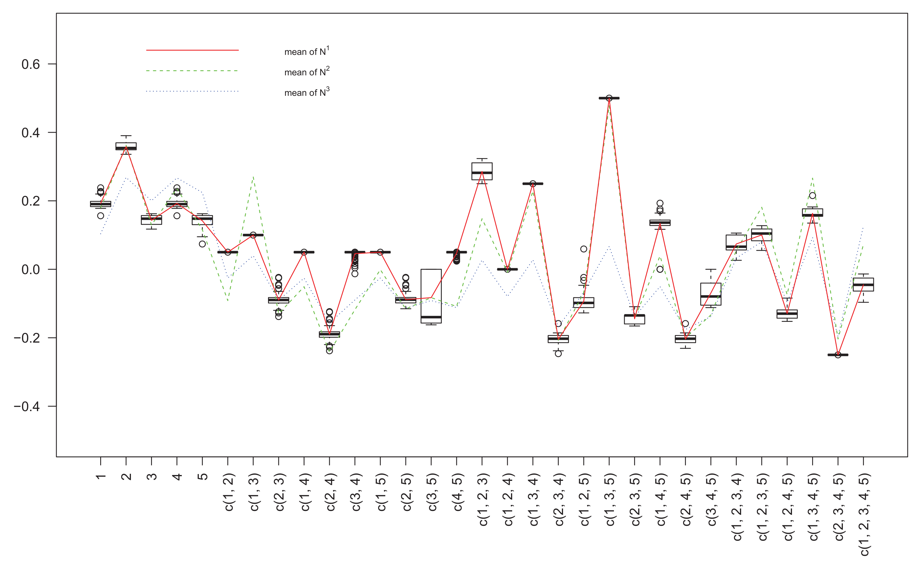
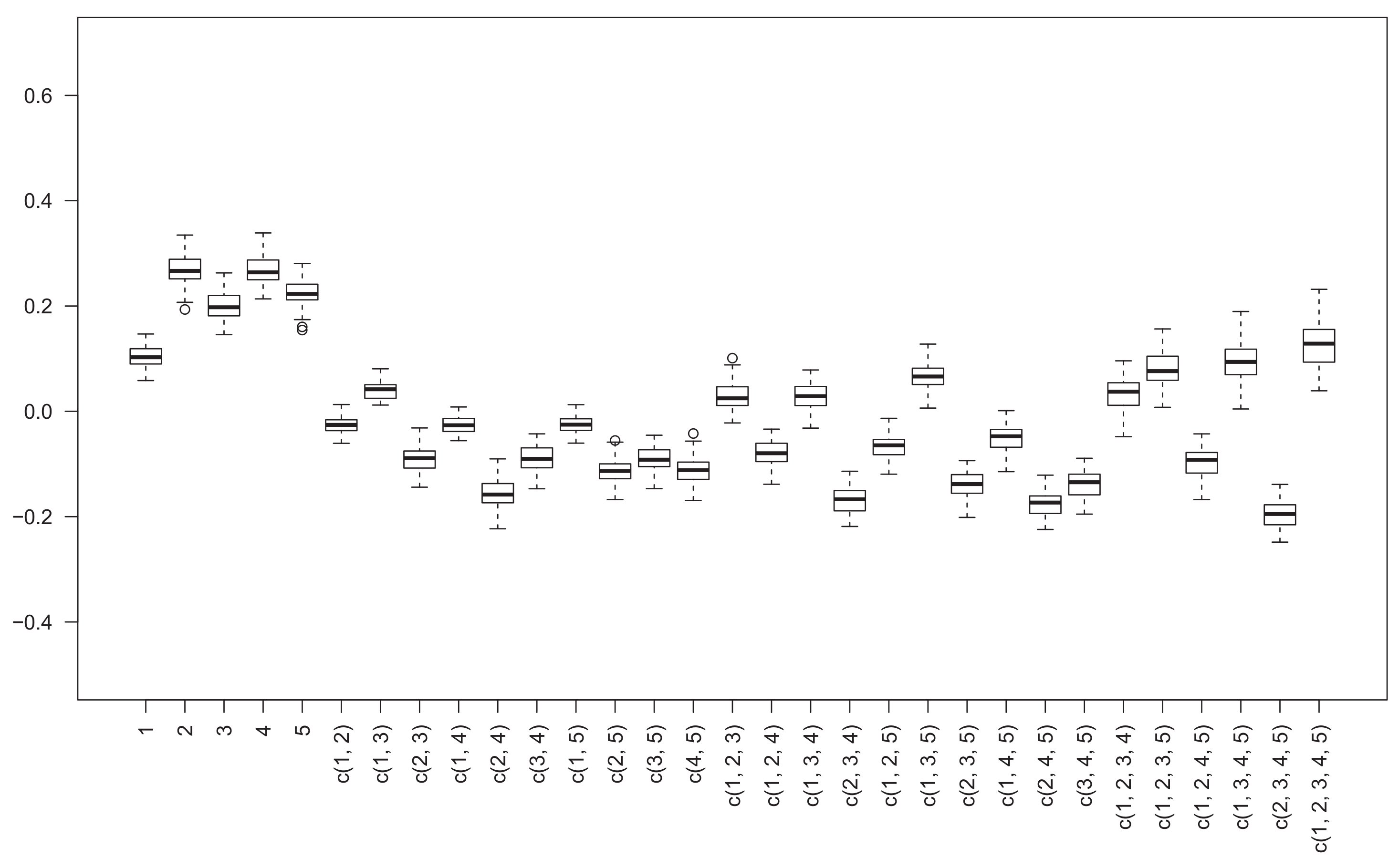
The matrices
,
and
are shown in
Figure 1,
Figure 2 and
Figure 3, and the column means of three matrices are also given in
Figure 1 for the purpose of comparison, where for the horizontal axis “c(1, 2)” means the coalition of decision criteria 1 and 2, i.e., {1, 2}. Taking nonadditivity index
as a reference (the solid lines), we can find out that the nonadditivity indices
and
have the same inflection trends, the positivity or negativity of almost all criteria subsets are the same, and especially on some subsets, e.g., {2, 3}, {2, 4}, {3, 5}, {2, 3, 5} and {1, 2, 4, 5}, three nonadditivity indices have very close values. Compared with
,
has a trend relatively more similar to
. From
Figure 2 and
Figure 3, we can get that nonadditivity index
has a relatively dispersive distribution, whereas
is more concentrative.
By executing the random simulation based comprehensive decision aid algorithm, Algorithm 2, with the three capacity matrices
,
and
, we can have the corresponding dominance relationships of all alternatives and three ranking orders as follows:
One can see that the ranking order from , compared with that from , relatively caters the ranking order from . Hence, if we take the random generation algorithm with mix constraints of nonadditivity index as a benchmark, Algorithm 3 can be a better choice than Algorithm 4 on the basis of comparison analysis of this example.
Finally, we should emphasise the major advantage of Algorithms 3 and 4: They do not need the sequential and taxing operations of the traditional random generation methods, such as construct preference constraints, establishment of the monotonicity conditions of all the set inclusion, checking and adjusting the inconsistency among the preference, choosing the selection principle of most satisfactory capacity and solving the optimization models of capacity identification. Hence, they are more efficient in dealing with a large scale of decision criteria and can accomplish relatively comprehensive decision making in practice.
6. Conclusions
In this paper, we proposed two quasi-random generation algorithms of capacity under the case of using the nonadditivity index to show the decision maker’s preference information. The nonadditivity index has some good mathematical properties and rather intuitive explanations on the interaction phenomenon of decision criteria, and it is also a competent and flexible tool to represent the complex interaction cases among criteria. These two types of nonadditivity index oriented quasi-random generation algorithms are not unblemished in rigorously fitting the decision preference but have an incomparable execution efficiency in practice on account of not involving the preference inconsistency checking and adjusting as well as the optimization model establishing and solving, which will be really helpful for efficiently dealing with a large scale decision making problem with deeply correlative criteria. Future research will focus on some effective measures to improve the fitting accuracy of nonadditivity oriented algorithms to the decision maker’s complicated preference as well as the random generation algorithm based decision aid packages.


