Abstract
The main goal of the paper is to introduce different models to calculate the amount of money that must be allocated to each stock in a statistical arbitrage technique known as pairs trading. The traditional allocation strategy is based on an equal weight methodology. However, we will show how, with an optimal allocation, the performance of pairs trading increases significantly. Four methodologies are proposed to set up the optimal allocation. These methodologies are based on distance, correlation, cointegration and Hurst exponent (mean reversion). It is showed that the new methodologies provide an improvement in the obtained results with respect to an equal weighted strategy.
1. Introduction
Efficient Market Hypothesis (EMH) is a well-known topic in finance. Implications of the weak form of efficiency is that information about the past is reflected in the market price of a stock and therefore, historical market data is not helpful for predicting the future. An investor in an efficient market will not be able to obtain a significant advantage over a benchmark portfolio or a market index trading based on historical data (for a review see Reference [1,2]).
On the opposite way, some researchers have shown that the use of historical data as well as trading techniques is sometimes possible due to temporal markets anomalies. Despite that most of economists consider that these anomalies are not compatible with an efficient market, recent papers have shown new perspectives called Fractal Market Hypothesis (FMH) and Adaptive Market Hypothesis (AMH), that tries to integrate market anomalies into the efficient market hypothesis.
The EMH was questioned by the mathematician Mandelbrot in 1963 and after the economist Fama showed his doubts about the Normal distribution of stock returns, essential point of the efficient hypothesis. Mandelbrot concluded that stock prices exhibit long-memory, and proposed a Fractional Brownian motion to model the market. Di Matteo [3,4] considered that investors can be distinguished by the investment horizons in which they operate. This consideration allows us to connect the idea of long memory and the efficiency hypothesis. In the context of an efficient market, the information is considered as a generic item. This means that the impact that public information has over each investor is similar. However, the FMH assumes that information and expectations affect in a different way to traders, which are only focused on short terms and long term investors [5,6].
The idea of a AMH has been recently introduced by Lo [7] to reflect an evolutionary perspective of the market. Under this new idea, markets show complex dynamics at different times which make that some arbitrage techniques perform properly in some periods and poorly in others.
In an effort of conciliation, Sanchez et al. [8] remarks that the market dynamic is the results of different investors interactions. In this way, scaling behavior patterns of a specific market can characterize it. Developed market price series usually show only short memory or no memory whereas emerging markets do exhibit long-memory properties. Following this line, in a recent contribution, Sanchez et al. [9] proved that pairs trading strategies are quite profitable in Latin American Stock Markets whereas in Nasdaq 100 stocks, it is only in high volatility periods. These results are in accordance with both markets hyphotesis. A similar result is obtained by Zhang and Urquhart [10] where authors are able to obtain a significant exceed return with a trading strategy across Mainland China and Hong kong but not when the trading is limited to one of the markets. The authors argue that this is because of the increasing in the efficiency of Mainland China stock market and the decreasing of the Hong Kong one because of the integration of Chinese stock markets and permission of short selling.
These new perspectives of market rules explain why statistical arbitrage techniques, such as pairs trading, can outperform market indexes if they are able to take advantage of market anomalies. In a previous paper, Ramos et al. [11] introduced a new pairs trading technique based on Hurst exponent which is the classic and well known indicator of market memory (for more details, References [8,12] contain an interesting review). For our purpose, the selection of the pair policy is to choose those pairs with the lowest Hurst exponent, that is, the more anti-persistent pairs. Then we use a reversion to the mean trading strategy with the more anti-persistent pairs according with the previously mentioned idea that developed market prices show short memory [3,13,14,15].
Pairs trading literature is extensive and mainly focused on the pair selection during the trading period as well as the developing of a trading strategy. The pioneer paper was Gatev et al. [16] where authors introduced the distance method with an application to the US market. In 2004, Vidyamurthy [17] presented the theoretical framework for pair selection using the cointegration method. Since then, different analysis have been carried out using this methodology in different markets, such us the European market [18,19], the DJIA stocks [20], the Brazilian market [21,22] or the STOXX 50 index [23]. Galenko et al. [24] made an application of the cointegration method to arbitrage in fund traded on different markets. Lin et al. [25] introduced the minimum profit condition into the trading strategy and Nath [26] used the cointegration method in intraday data. Elliott et al. [27] used Markov chains to study a mean reversion strategy based on differential predictions and calibration from market observations. The mean reversion approach has been tested in markets not considered efficient such us Asian markets [28] or Latin American stock markets [9]. A recent contribution of Ramos et al. [29] introduced a new methodology for testing the co-movement between assets and they tested it in statistical arbitrage. However, researchers did not pay attention to the amount of money invested in every asset, considering always a null dollar market exposition. This means that when one stock is sold, the same amount of the other stock is purchased. In this paper we propose a new methodology to improve pairs trading performance by developing new methods to improve the efficiency in calculating the ratio to invest in each stock that makes up the pair.
2. Pair Selection
One of the topics in pairs trading is how to find a suitable pair for pairs trading. Several methodologies have been proposed in the literature, but the more common ones are co-movement and the distance method.
2.1. Co-Movement
Baur [30] defines co-movement as the shared movement of all assets at a given time and it can be measured using correlation or cointegration techniques.
Correlation technique is quite simple, and the higher the correlation coefficient is, the greatest they move in sync. An important issue to be considered is that correlation is intrinsically a short-run measure, which implies that a correlation strategy will work better with a lower frequency trading strategy.
In this work, we will use the Spearman correlation coefficient, which is a nonparametric range statistic which measure the relationship between two variables. This coefficient is particularly useful when the relationship between the two variables is described by a monotonous function, and does not assume any particular distribution of the variables [31].
The Spearman correlation coefficient for a sample , of size n can be described as follows: first, consider the ranks of the samples , , then the Spearman correlation coefficient is calculated as:
where
- denotes the Pearson correlation coefficient, applied to the rank variables
- , is the covariance of the rank variables.
- and , are the standard deviations of the rank variables.
Cointegration approach was introduced by Engle and Granger [32] and it considers a different type of co-movement. In this case, cointegration refers to movements in prices, not in returns, so cointegration and correlation are related, but different concepts. In fact, cointegrated series can perfectly be low correlated.
Two stocks A and B are said to be cointegrated if there exists such that is a stationary process, where and are the log-prices A and B, respectively. In this case, the following model is considered:
where
- is the mean of the cointegration model
- is the cointegration residual, which is a stationary, mean-reverting process
- is the cointegration coefficient.
We will use the ordinary least squares (OLS) method to estimate the regression parameters. Through the Augmented Dickey Fuller test, we will verify if the residual is stationary or not, and with it we will check if the stocks are co-integrated.
2.2. The Distance Method
This methodology was introduced by Gatev et al. [16]. It is based on minimizing the sum of squared differences between somehow normalized price series:
where is the cumulative return of stock A at time t and is the cumulative return of stock B at time t.
The best pair will be the pair whose distance between its stocks is the lowest possible, since this means that the stocks moves in sync and there is a high degree of co-movement between them.
An interesting contribution to this trading system was introduced by Do and Faff [33,34]. The authors replicated this methodology for the U.S. CRSP stock universe and an extended period. The authors confirmed a declining profitability in pairs trading as well as the unprofitability of the trading strategy due to the inclusion of trading costs. Do and Faff then refined the selection method to improve the pair selection. The authors restricted the possible combinations only within the 48 Fama-French industries and they looked for pairs with a high number of zero-crossings to favor the pairs with greatest mean-reversion behavior.
2.3. Pairs Trading Strategy Based on Hurst Exponent
Hurst exponent (H from now on) was introduced by Hurst in 1951 [35] to deal with the problem of reservoir control for the Nile River Dam. Until the beginning of the 21st century, the most common methodology to estimate H was the R/S analysis [36] and the DFA [37], but due to accuracy problems remarked by several studies (see for example References [38,39,40,41]), new algorithms were developed for a more efficient estimation of the Hurst exponent, some of them with its focus on financial time series. One of the most important methodologies is the GHE algorithm, introduced in Reference [42], which is a general algorithm with good properties.
The GHE is based on the scaling behavior of the statistic
which is given by
where is the scale (usually chosen between 1 and a quarter of the length of the series), H is the Hurst exponent, denotes the sample average on time t and q is the order of the moment considered. In this paper we will always use .
The GHE is calculated by linear regression, taking logarithms in the expression contained in (4) for different values of [3,43].
The interpretation of H is as follow: when H is greater than , the process is persistent, when H is less than , it is anti persistent, while Brownian motion has a value of H equal to .
With this technique, pairs with the lowest Hurst exponent has to be chosen in order to apply reversion to the mean strategies which is also the base of correlation and cointegration strategies.
2.4. Pairs Trading Strategy
Next, we describe the pairs trading strategy, which is taken from Reference [11]. As usual, we consider two periods. The first one is the formation period (one year), which is used for the pair selection. This is done using the four methods defined in this section (distance, correlation, cointegration and Hurst exponent). The second period is the execution period (six months), in which all selected pairs are traded as follows:
- In case the pair will be sold. The position will be closed if or .
- In case the pair will be bought. The position will be closed if or .
where m is a moving average of the series of the pair and s is a moving standard deviation of m.
3. Forming the Pair: Some New Proposals
As we remarked previously, all works assume that the amount purchased in a stock is equal to the amount sold in the other pair component. The main contribution of this paper is to analyse if not assuming an equal weight ratio in the formation of the pair improves the performance of the different pair trading strategies. In this section different methods are proposed.
When a pair is formed, we use two stocks A and B. This two stocks have to be normalized somehow, so we introduce a constant b such that stock A is comparable to stock . Then, to buy an amount T of the pair means that we buy of stock A and sell of stock B, while to sell an amount T of the pair means that we sell of stock A and buy of stock B.
We will denote by the logarithm of the price of stock X in time t minus the logarithm of the price of stock X at time , that is , and by the log-return of stock X between times and t, .
In this paper we discuss the following ways to calculate the weight factor b:
- 1.
- Equal weight ().In this case . This is the way used in most of the literature. In this case, the position in the pair is dollar neutral. This method was used in Reference [16], and since then, it has become the more popular procedure to fix b.
- 2.
- Based on volatility.Volatility of stock A is and volatility of stock B is . If we want that A and have the same volatility then . This approach was used in Reference [11] and it is based on the idea that both stocks are normalized if they have the same volatility.
- 3.
- Based on minimal distance of the log-prices.In this case we minimize the function , so we look for the weight factor b such that and has the minimum distance. This approach is based on the same idea that the distance as a selection method. The closer is the evolution of the log-price of stocks A and , the more reverting to the mean properties the pair will have.
- 4
- Based on correlation of returns.If returns are correlated then is approximately equal to , where b is obtained by linear regression . In this case, if returns of stocks A and B are correlated, then the distribution of and will be the same, so we can use this b to normalize both stocks.
- 5.
- Based on cointegration of the prices.If the prices (in fact, the log-prices) of both stocks A and B are cointegrated then is stationary, whence b is obtained by linear regression . In this case, this value of b makes the pair series stationary so we can expect reversion to the mean properties of the pair series. Even if the stocks A and B are not perfectly cointegrated, this method for the calculation of b may be still valid, since, thought may be not stationary, it can be somehow close to it or still have mean-reversion properties.
- 6.
- Based on lowest Hurst exponent of the pair.The series of the pair is defined as . In this case, we look for the weight factor b such that the series of the pair has the lowest Hurst exponent, what implies that the series is as anti-persistent as possible. So we look for b which minimizes the function , where is the Hurst exponent of the pair series . The idea here is similar to the cointegration method, but from a theoretical point of view, we do not expect to be stationary (which is quite difficult with real stocks), but to be anti-persistent, which is enough for our trading strategy.
4. Experimental Results
For testing the results through the different models introduced in this paper, we will use the components of the Nasdaq 100 index technological sector (see Table A1 in Appendix A),for the period between January 1999 and December 2003, coinciding with the “dot.com” bubble crash and the period between January 2007 and December 2012, this period coincides with the financial instability caused by the “subprime” crisis. These periods are choosen based on the results showed by Sánchez et al. [9].
We use Pairs Trading traditional methods (Distance Method, Correlation and Cointegration) in addition to the method developed by Ramos et al. [11] based on the Hurst exponent.
In Appendix B, it is shown the results obtained for different selection methods and different ways to calculate b, for the two selected periods. In addition to the returns obtained for each portfolio of pairs, we include two indicators of portfolio performance and risk, the Sharpe Ratio and the maximum Drawdown.
In the first period analyzed, the method to calculate b is never the best one. The best methods to calculate b seems to be the cointegration method and the minimization of the Hurst exponent. Also note that the Spearman correlation, the cointegration and the Hurst exponent selection methods provide strategies with high Sharpe ratios for several methods to calculate b.
In the second period analyzed, the method to calculate b works fine with the cointegration selection method, but it is not so good with the other ones, while the correlation method to calculate b is often one of the best ones.
Note that, in both periods, the Sharpe ratio when we use to calculate b are usually quite low with respect to the other methods.
Figure 1, Figure 2, Figure 3 and Figure 4 show the cumulative log-return of the strategy for different selection methods and different ways to calculate b.
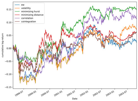
Figure 1.
Comparative portfolio composed of 30 pairs using cointegration method for selection during the period 1999–2003.
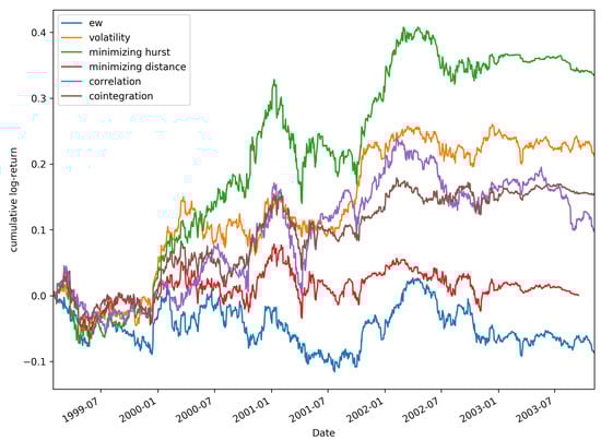
Figure 2.
Comparative portfolio composed of 20 pairs using the Hurst exponent method for selection during the period 1999–2003.
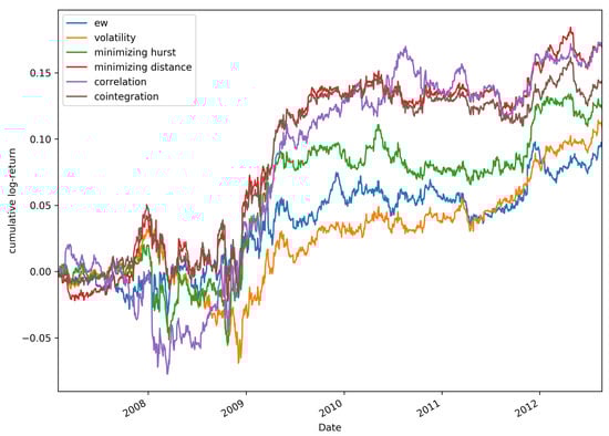
Figure 3.
Comparative portfolio composed of 20 pairs using distance method for selection during the period 2007–2012.
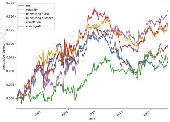
Figure 4.
Comparative portfolio composed of 10 pairs using Spearman method for selection during the period 2007–2012.
Figure 1 shows the returns obtained for the period 1999–2003 using the co-integration approach as a selection method. We can observe that during the whole period, the best option is to choose to calculate the b factor by means of the lowest value of the Hurst exponent, while the method is the worst.
Figure 2 represents the returns obtained for each of the b calculation methods for the 1999–2003 period, using the Hurst exponent method for the selection of pairs and a portfolio composed of 20 pairs. It can be observed that during the period studied, the results obtained using the method are also negative, while the Hurst exponent method is again the best option.
For the period 2007–2012, for a portfolio composed of 20 pairs selected using the distance method, Figure 3 shows the cumulative returns for the different methods proposed. In this case we can highlight the methods of correlation, minimizing distance and cointegration, as the methods to calculate b that provide the highest returns. Again, we can observe that the worst options would be the method together with the volatility one.
Figure 4 shows the results obtained using the different models to calculate the b factor for a portfolio of 10 pairs by selecting them using the Spearman model. We can observe that all returns are positive throughout the period studied (2007–2012). The most outstanding are the methods of correlation, minimum distance and volatility, which move in a very similar way during this period. On the contrary, the method of the lowest value of the Hurst exponent and the one are the worst options during the whole period.
Finally, we complete our sensitivity analysis by analyzing the influence of the strategy considered in Section 2.4. We consider the Hurst exponent as the selection method, 20 pairs in the portfolio and the period 1999–2003. We change the strategy by using 1 (as before), 1.5 and 2 standard deviations. That is, we modify the strategy as follows:
- In case the pair will be sold. The position will be closed if or .
- In case the pair will be bought. The position will be closed if or .
where . Table A2 shows that the , correlation and minimal distance obtain the worst results, while cointegration and the Hurst exponent obtain robust and better results for the different values of k.
Discussion of the Results
In Table A3, Table A4, Table A5, Table A6, Table A7, Table A8, Table A9 and Table A10, the results obtained with a pair trading strategy are shown. In those tables, we have consider four different methods for the pair selection (distance, correlation, cointegration and Hurst exponent), three different number of pairs (10, 20 and 30 pairs) and two periods (1999–2003 and 2007–2012). Overall, if we focus on the Sharpe ratio of the results, in of the cases (14 out of 24) the method for calculating b obtains one of the three (out of seven) worst results. If we compare the method with the other methods proposed we obtain the following: minimal Hurst exponent is better than in of the cases, minimal distance is better than in of the cases, correlation is better than in of the cases, cointegration is better than in of the cases and volatility is better than in of the cases. So, in general, the proposed methods (except the volatility one) tend to be better than the one.
However, since we are considering stocks in the technology sector, if we focus in the dot.com bubble (that is, the period 1999–2003) which affected more drastically to the stocks in the portfolio, we have, considering the Sharpe ratio of the results, that in of the cases (10 out of 12) the method for calculating b obtains one of the three (out of seven) worst results. In this period, if we compare the method with the other methods proposed we obtain the following: minimal Hurst exponent is better than in of the cases, minimal distance is better than in of the cases, correlation is better than in of the cases, cointegration is better than in of the cases and volatility is better than in of the cases. So, in general, the proposed methods (except the volatility one) tend to be much better than the one in this period.
On the other hand, in the second period (2007–2012), the performs much better than in the first period (1999–2003) and it does similarly or slightly better than the other methods.
Results show that these novel approaches used to calculate the factor b improve the results obtained compared with the classic method for the different strategies and mainly in the first period considered (1999–2003). Therefore, it seems that the performance of pairs trading can be improved not only acting on the strategy, but also on the method for the allocation in each stock.
In this section we have tested different methods for the allocation in each stock of the pair. Though we have used the different allocation methods with all the selection methods analyzed, it is clear that some combinations make more sense than others. For example, if the selection of the pair is done by selecting the pair with a lower Hurst exponent, the allocation method based on the minimization of the Hurst exponent of the pair should work better than other allocation methods.
One of the main goal of this paper is to point out that the allocation in each stock of the pair can be improved in the pairs trading strategy and we have given some ways to make this allocation. However, further research is needed to asses which of the methods is the best for this purpose. Even better, which of the combinations of selection and allocation method is the best. Though this problem depends on many factors, and some of them changes, depending on investor preferences, a multi-criteria decision analysis (see, for example References [44,45,46]) seems to be a good approach to deal with it.
In fact, in future research it can be tested if the selection method can be improved if we take into account the allocation method. For example, for the distance selection method, we can use the allocation method based on the minimization of the distance to normalize the price of the stocks in a different way than in the classical distance selection method, taking into account the allocation in each stock. Not all selection methods can be improved in this way (for example, the correlation selection method will not improve), but some of them, including some methods which we have not analyzed in this paper or future selection methods, could be improved.
5. Conclusions
In pairs trading literature, researchers have focused their attention in increasing pairs trading performance proposing different methodologies for pair selection. However, in all cases it is assumed that the amount invested in each stock of a pair (b) must be equal. This technique is called Equally Weighted ().
This paper presents a novel approach to try to improve the performance of this statistical arbitrage technique through novel methodologies in the calculation of b. Any selection method can benefit from these new allocation methods. Depending on the selection method used, we prove that the new methodologies for calculating the factor b obtain a greater return than those used up to the present time.
Results show that the classic EW method does not performance as well as the others. Cointegration, correlation and Hurst exponent give excellent results when are used to calculate factor b.
Author Contributions
Conceptualization, J.P.R.-R., J.E.T.-S. and M.Á.S.-G.; Methodology, J.P.R.-R., J.E.T.-S. and M.Á.S.-G.; Software, J.P.R.-R., J.E.T.-S. and M.Á.S.-G.; Validation, J.P.R.-R., J.E.T.-S. and M.Á.S.-G.; Formal Analysis, J.P.R.-R., J.E.T.-S. and M.Á.S.-G.; Investigation, J.P.R.-R., J.E.T.-S. and M.Á.S.-G.; Resources, J.P.R.-R., J.E.T.-S. and M.Á.S.-G.; Data Curation, J.P.R.-R., J.E.T.-S. and M.Á.S.-G.; Writing–Original Draft Preparation, J.P.R.-R., J.E.T.-S. and M.Á.S.-G.; Writing–Review & Editing, J.P.R.-R., J.E.T.-S. and M.Á.S.-G.; Visualization, J.P.R.-R., J.E.T.-S. and M.Á.S.-G.; Supervision, J.P.R.-R., J.E.T.-S. and M.Á.S.-G.; Project Administration, J.P.R.-R., J.E.T.-S. and M.Á.S.-G.; Funding Acquisition, J.P.R.-R., J.E.T.-S. and M.Á.S.-G. All authors have read and agreed to the published version of the manuscript.
Funding
Juan Evangelista Trinidad-Segovia is supported by grant PGC2018-101555-B-I00 (Ministerio Español de Ciencia, Innovación y Universidades and FEDER) and UAL18-FQM-B038-A (UAL/CECEU/FEDER). Miguel Ángel Sánchez-Granero acknowledges the support of grants PGC2018-101555-B-I00 (Ministerio Español de Ciencia, Innovación y Universidades and FEDER) and UAL18-FQM-B038-A (UAL/CECEU/FEDER) and CDTIME.
Conflicts of Interest
The authors declare no conflict of interest. The funders had no role in the design of the study; in the collection, analyses, or interpretation of data; in the writing of the manuscript, or in the decision to publish the results.
Appendix A. Stocks Portfolio Technology Sector Nasdaq 100

Table A1.
The Technology Sector Nasdaq 100.
Table A1.
The Technology Sector Nasdaq 100.
| Ticker | Company |
|---|---|
| AAPL | Apple Inc. |
| ADBE | Adobe Systems Incorporated |
| ADI | Analog Devices, Inc. |
| ADP | Automatic Data Processing, Inc. |
| ADSK | Autodesk, Inc. |
| AMAT | Applied Materials, Inc. |
| ATVI | Activision Blizzard, Inc. |
| AVGO | Broadcom Limited |
| BIDU | Baidu, Inc. |
| CA | CA, Inc. |
| CERN | Cerner Corporation |
| CHKP | Check Point Software Technologies Ltd. |
| CSCO | Cisco Systems, Inc. |
| CTSH | Cognizant Technology Solutions Corporation |
| CTXS | Citrix Systems, Inc. |
| EA | Electronic Arts Inc. |
| FB | Facebook, Inc. |
| FISV | Fiserv, Inc. |
| GOOG | Alphabet Inc. |
| GOOGL | Alphabet Inc. |
| INTC | Intel Corporation |
| INTU | Intuit Inc. |
| LRCX | Lam Research Corporation |
| MCHP | Microchip Technology Incorporated |
| MSFT | Microsoft Corporation |
| MU | Micron Technology, Inc. |
| MXIM | Maxim Integrated Products, Inc. |
| NVDA | NVIDIA Corporation |
| QCOM | QUALCOMM Incorporated |
| STX | Seagate Technology plc |
| SWKS | Skyworks Solutions, Inc. |
| SYMC | Symantec Corporation |
| TXN | Texas Instruments Incorporated |
| VRSK | Verisk Analytics, Inc. |
| WDC | Western Digital Corporation |
| XLNX | Xilinx, Inc. |
Appendix B. Empirical Results
For each model (Equal Weight, Volatility, Minimal Distance of the log-prices, Correlation of returns, Cointegration of the prices, lowest Hurst exponent of the pair), we have considered 3 scenarios, depending on the amount of pairs included in the portfolio.
- 1.
- Number of standard deviations.
Table A2. Comparison of results using the Hurst exponent selection method for the period 1999–2003 with 20 pairs and different numbers of standard deviations.Table A2. Comparison of results using the Hurst exponent selection method for the period 1999–2003 with 20 pairs and different numbers of standard deviations.
b Calculation Method k Sharpe Profit TC Cointegration 1.0 0.39 14.55% Cointegration 1.5 0.60 26.00% Cointegration 2.0 0.59 24.08% Correlation 1.0 0.15 6.10% Correlation 1.5 0.17 8.21% Correlation 2.0 0.31 13.82% EW 1.0 −0.28 −11.25% EW 1.5 0.38 15.49% EW 2.0 0.21 7.74% Lowest Hurst Exponent 1.0 0.70 40.51% Lowest Hurst Exponent 1.5 0.51 28.00% Lowest Hurst Exponent 2.0 0.57 28.51% Minimal Distance 1.0 0.03 0.05% Minimal Distance 1.5 0.39 15.70% Minimal Distance 2.0 0.31 11.48% Volatility 1.0 0.49 18.22% Volatility 1.5 0.41 16.37% Volatility 2.0 0.25 9.12% number of standard deviations; Sharpe Ratio; Profitability with transaction costs. - 2.
- Distance (1999–2003).
Table A3. Comparison of results using the distance selection method for the period 1999–2003.Table A3. Comparison of results using the distance selection method for the period 1999–2003.
b Calculation Method N Oper AR %Profit TC Sharpe Max Drawdown Cointegration 10 1375 0.40% 0.72% 0.05 13.70% Correlation 10 1357 −0.60% −4.36% −0.07 18.60% EW 10 1403 −1.30% −7.30% −0.15 19.60% Minimal distancie 10 1389 −0.90% −5.49% −0.10 16.30% Lowest Hurst Exponent 10 1352 −1.50% −8.55% −0.16 19.20% Volatility 10 1370 −1.30% −7.57% −0.16 13.90% Cointegration 20 2786 3.50% 16.31% 0.47 7.40% Correlation 20 2630 2.80% 12.68% 0.36 9.20% EW 20 2884 1.00% 3.36% 0.14 12.30% Minimal distancie 20 2794 2.50% 11.00% 0.34 8.30% Lowest Hurst Exponent 20 2685 0.60% 1.66% 0.08 12.00% Volatility 20 2812 0.40% 0.39% 0.06 8.70% Cointegration 30 4116 2.80% 12.83% 0.42 8.00% Correlation 30 3830 2.00% 8.62% 0.27 12.60% EW 30 4247 1.10% 4.18% 0.18 14.80% Minimal distancie 30 4105 1.90% 7.93% 0.28 8.40% Lowest Hurst Exponent 30 3861 0.30% 0.01% 0.04 11.80% Volatility 30 4160 0,10% -0,99% 0.01 9,20% Number of pairs; Number of operations; Annualised return; Profitability with transaction costs; Sharpe Ratio. - 3.
- Distance (2007–2012).
Table A4. Comparison of results using the distance selection method for the period 2007–2012.Table A4. Comparison of results using the distance selection method for the period 2007–2012.
b Calculation Method N Oper AR %Profit TC Sharpe Max Drawdown Cointegration 10 1666 1.80% 8.73% 0.35 10.20% Correlation 10 1594 3.50% 19.51% 0.55 12.10% EW 10 1677 1.20% 5.42% 0.22 9.40% Minimal distance 10 1649 2.80% 15.15% 0.56 8.80% Lowest Hurst Exponent 10 1677 2.60% 13.42% 0.51 8.00% Volatility 10 1684 1.20% 5.22% 0.24 11.90% Cointegration 20 3168 2.60% 13.82% 0.60 6.50% Correlation 20 2985 3.10% 16.91% 0.58 9.30% EW 20 3219 1.70% 8.19% 0.36 4.20% Minimal distance 20 3172 3.10% 17.01% 0.72 6.20% Lowest Hurst Exponent 20 3116 2.20% 11.54% 0.51 7.20% Volatility 20 3221 2.00% 9.89% 0.48 10.00% Cointegration 30 4714 1.50% 7.33% 0.38 6.70% Correlation 30 4453 1.40% 6.42% 0.29 10.90% EW 30 4791 1.40% 6.50% 0.34 5.30% Minimal distance 30 4709 1.70% 8.43% 0.44 5.90% Lowest Hurst Exponent 30 4545 1.40% 6.48% 0.35 6.80% Volatility 30 4785 1.60% 7.60% 0.43 9.00% Number of pairs; Number of operations; Annualised return; Profitability with transaction costs; Sharpe Ratio. - 4.
- Spearman Correlation (1999–2003).
Table A5. Comparison of results using the Spearman correlation selection method for the period 1999–2003.Table A5. Comparison of results using the Spearman correlation selection method for the period 1999–2003.
b Calculation Method N Oper AR %Profit TC Sharpe Max Drawdown Cointegration 10 1274 4.10% 19.93% 0.50 14.30% Correlation 10 1432 3.00% 13.67% 0.36 11.20% EW 10 1400 4.30% 20.80% 0.56 9.30% Minimal distance 10 1219 4.00% 19.68% 0.51 12.50% Lowest Hurst Exponent 10 1103 5.70% 29.20% 0.64 10.70% Volatility 10 1405 3.30% 15.39% 0.45 8.40% Cointegration 20 2583 4.70% 23.41% 0.69 12.30% Correlation 20 2833 3.90% 18.78% 0.55 10.90% EW 20 2814 2.80% 12.69% 0.45 8.30% Minimal distance 20 2538 4.40% 21.63% 0.65 12.50% Lowest Hurst Exponent 20 2176 3.50% 16.71% 0.48 10.40% Volatility 20 2781 2.50% 11.01% 0.41 9.30% Cointegration 30 3776 4.90% 24.54% 0.79 8.10% Correlation 30 4196 2.80% 12.90% 0.41 8.60% EW 30 4168 0.40% 0.71% 0.08 9.90% Minimal distance 30 3717 4.20% 20.76% 0.69 8.30% Lowest Hurst Exponent 30 3236 4.20% 20.72% 0.56 8.20% Volatility 30 4125 1.20% 4.52% 0.22 9.50% Number of pairs; Number of operations; Annualised return; Profitability with transaction costs; Sharpe Ratio. - 5.
- Spearman Correlation (2007–2012).
Table A6. Comparison of results using the Spearman correlation selection method for the period 2007–2012.Table A6. Comparison of results using the Spearman correlation selection method for the period 2007–2012.
b Calculation Method N Oper AR %Profit TC Sharpe Max Drawdown Cointegration 10 1614 1.70% 8.09% 0.38 8.30% Correlation 10 1653 2.90% 15.75% 0.75 4.60% EW 10 1620 1.20% 5.28% 0.37 7.00% Minimal distancie 10 1551 2.50% 13.05% 0.58 7.80% Lowest Hurst Exponent 10 1117 1.30% 6.18% 0.42 4.20% Volatility 10 1668 2.30% 12.13% 0.72 5.00% Cointegration 20 3022 1.00% 4.09% 0.29 6.80% Correlation 20 3268 2.60% 13.77% 0.75 4.00% EW 20 3236 1.40% 6.78% 0.46 5.70% Minimal distance 20 2944 1.10% 4.93% 0.34 7.80% Lowest Hurst Exponent 20 1966 0.40% 1.12% 0.14 3.90% Volatility 20 3282 1.30% 5.76% 0.42 4.70% Cointegration 30 4342 0.80% 3.15% 0.27 5.80% Correlation 30 4872 2.60% 13.58% 0.74 4.30% EW 30 4814 1.60% 7.80% 0.57 4.90% Minimal distance 30 4222 0.90% 3.69% 0.30 7.00% Lowest Hurst Exponent 30 2718 0.60% 2.49% 0.26 2.80% Volatility 30 4864 1.90% 9.28% 0.67 3.60% Number of pairs; Number of operations; Annualised return; Profitability with transaction costs; Sharpe Ratio. - 6.
- Cointegration (1999–2003).
Table A7. Comparison of results using the cointegration selection method for the period 1999–2003.Table A7. Comparison of results using the cointegration selection method for the period 1999–2003.
b Calculation Method N Oper AR %Profit TC Sharpe Max Drawdown Cointegration 10 998 5.30% 26.80% 0.58 12.40% Correlation 10 1015 7.30% 39.38% 0.78 9.30% EW 10 1369 4.30% 20.83% 0.41 10.30% Minimal distance 10 945 4.00% 19.45% 0.47 9.40% Lowest Hurst Exponent 10 1123 7.70% 41.68% 0.79 11.90% Volatility 10 1376 6.90% 36.62% 0.68 11.00% Cointegration 20 1984 5.50% 28.41% 0.78 9.00% Correlation 20 1985 5.50% 28.31% 0.76 6.40% EW 20 2718 2.90% 13.24% 0.36 9.90% Minimal distance 20 1876 4.50% 22.36% 0.67 8.10% Lowest Hurst Exponent 20 2031 6.90% 36.88% 0.90 7.70% Volatility 20 2688 4.10% 19.76% 0.50 11.50% Cointegration 30 2957 0.90% 3.51% 0.14 11.00% Correlation 30 3132 2.40% 11.06% 0.36 10.30% EW 30 4064 −0.10% −1.85% −0.01 12.20% Minimal distance 30 2783 0.70% 2.67% 0.12 9.40% Lowest Hurst Exponent 30 2924 3.60% 17.23% 0.50 7.50% Volatility 30 4040 0.90% 3.25% 0.12 13.00% Number of pairs; Number of operations; Annualised return; Profitability with transaction costs; Sharpe Ratio. - 7.
- Cointegration (2007–2012).
Table A8. Comparison of results using the cointegration selection method for the period 2007–2012.Table A8. Comparison of results using the cointegration selection method for the period 2007–2012.
b Calculation Method N Oper AR %Profit TC Sharpe Max Drawdown Cointegration 10 1516 −1.00% −6.82% −0.19 15.50% Correlation 10 1512 −0.10% −2.11% −0.02 14.70% EW 10 1604 1.40% 6.80% 0.30 9.60% Minimal distance 10 1478 0.70% 2.32% 0.12 12.50% Lowest Hurst Exponent 10 1502 −1.60% −9.90% −0.32 10.90% Volatility 10 1635 −0.10% −2.14% −0.02 12.90% Cointegration 20 2884 −0.70% −5.44% −0.19 9.90% Correlation 20 2955 −0.70% −5.28% −0.16 11.70% EW 20 3195 1.80% 8.90% 0.48 4.40% Minimal distance 20 2709 0.20% −0.15% 0.06 9.50% Lowest Hurst Exponent 20 2666 −0.90% −6.53% −0.26 9.00% Volatility 20 3189 0.50% 1.31% 0.14 8.90% Cointegration 30 4142 0.00% −1.38% 0.00 8.80% Correlation 30 4373 0.20% −0.56% 0.04 9.50% EW 30 4720 2.70% 14.63% 0.75 4.90% Minimal distance 30 3923 1.10% 4.69% 0.28 7.90% Lowest Hurst Exponent 30 3694 −0.30% −2.93% −0.09 7.60% Volatility 30 4742 1.30% 5.82% 0.36 7.00% Number of pairs; Number of operations; Annualised return; Profitability with transaction costs; Sharpe Ratio. - 8.
- Hurst exponent (1999–2003).
Table A9. Comparison of results using the Hurst exponent selection method for the period 1999–2003.Table A9. Comparison of results using the Hurst exponent selection method for the period 1999–2003.
b Calculation Method N Oper AR %Profit TC Sharpe Max Drawdown Cointegration 10 1136 −0.60% −3.94% −0.06 15.60% Correlation 10 1176 0.50% 1.32% 0.04 24.40% EW 10 1334 2.80% 12.87% 0.29 12.20% Minimal distance 10 1166 −1.20% −6.87% −0.12 13.50% Lowest Hurst Exponent 10 1234 4.60% 22.77% 0.37 21.40% Volatility 10 1401 7.40% 39.60% 0.72 14.40% Cointegration 20 2104 3.10% 14.55% 0.39 11.10% Correlation 20 2400 1.50% 6.10% 0.15 15.70% EW 20 2695 -2.10% −11.25% −0.28 12.30% Minimal distance 20 2093 0.20% 0.05% 0.03 10.60% Lowest Hurst Exponent 20 2375 7.50% 40.51% 0.70 17.10% Volatility 20 2755 3.80% 18.22% 0.49 8.90% Cointegration 30 2984 3.10% 14.91% 0.48 7.80% Correlation 30 3516 2.00% 8.83% 0.22 16.50% EW 30 4066 −1.30% −7.56% −0.19 11.80% Minimal distance 30 2915 2.70% 12.63% 0.41 6.50% Lowest Hurst Exponent 30 3411 7.10% 37.86% 0.78 13.40% Volatility 30 3994 4.40% 21.57% 0.63 6.50% Number of pairs; Number of operations; Annualised return; Profitability with transaction costs; Sharpe Ratio. - 9.
- Hurst exponent (2007–2012).
Table A10. Comparison of results using the Hurst exponent selection method for the period 2007–2012.Table A10. Comparison of results using the Hurst exponent selection method for the period 2007–2012.
b Calculation Method N Oper AR %Profit TC Sharpe Max Drawdown Cointegration 10 1596 3.00% 16.40% 0.55 8.00% Correlation 10 1587 3.70% 21.51% 0.57 9.80% EW 10 1643 3.00% 16.26% 0.59 9.10% Minimal distancie 10 1581 2.10% 11.02% 0.41 8.70% Lowest Hurst Exponent 10 1649 4.80% 28.15% 0.83 8.30% Volatility 10 1724 1.30% 5.98% 0.27 8.40% Cointegration 20 2795 0.80% 3.40% 0.21 7.10% Correlation 20 3001 2.60% 14.10% 0.50 7.50% EW 20 3258 1.70% 8.27% 0.40 9.10% Minimal distancie 20 2758 −0.40% −3.48% −0.10 10.60% Lowest Hurst Exponent 20 3129 1.90% 9.84% 0.39 8.30% Volatility 20 3204 0.40% 0.90% 0.11 6.40% Cointegration 30 4100 −0.20% −2.27% −0.05 9.30% Correlation 30 4418 2.00% 10.23% 0.43 8.10% EW 30 4666 1.90% 9.34% 0.46 7.60% Minimal distancie 30 4049 0.00% −1.55% −0.01 10.50% Lowest Hurst Exponent 30 4248 0.40% 0.78% 0.09 9.20% Volatility 30 4790 0.60% 1.50% 0.15 8.40% Number of pairs; Number of operations; Annualised return; Profitability with transaction costs; Sharpe Ratio.
References
- Fama, E. Efficient capital markets: II. J. Financ. 1991, 46, 1575–1617. [Google Scholar] [CrossRef]
- Dimson, E.; Mussavian, M. A brief history of market efficiency. Eur. Financ. Manag. 1998, 4, 91–193. [Google Scholar] [CrossRef]
- Di Matteo, T.; Aste, T.; Dacorogna, M.M. Using the scaling analysis to characterize their stage of development. J. Bank. Financ. 2005, 29, 827–851. [Google Scholar] [CrossRef]
- Di Matteo, T. Multi-scaling in finance. Quant. Financ. 2007, 7, 21–36. [Google Scholar] [CrossRef]
- Peters, E.E. Chaos and Order in the Capital Markets. A New View of Cycle, Prices, and Market Volatility; Wiley: New York, NY, USA, 1991. [Google Scholar]
- Peters, E.E. Fractal Market Analysis: Applying Chaos Theory to Investment and Economics; Wiley: New York, NY, USA, 1994. [Google Scholar]
- Lo, A.W. The adaptive markets hypothesis: Market efficiency from an evolutionary perspective. J. Portf. Manag. 2004, 30, 15–29. [Google Scholar] [CrossRef]
- Sanchez-Granero, M.A.; Trinidad Segovia, J.E.; García, J.; Fernández-Martínez, M. The effect of the underlying distribution in Hurst exponent estimation. PLoS ONE 2015, 28, e0127824. [Google Scholar]
- Sánchez-Granero, M.A.; Balladares, K.A.; Ramos-Requena, J.P.; Trinidad-Segovia, J.E. Testing the efficient market hypothesis in Latin American stock markets. Phys. A Stat. Mech. Its Appl. 2020, 540, 123082. [Google Scholar] [CrossRef]
- Zhang, H.; Urquhart, A. Pairs trading across Mainland China and Hong Kong stock Markets. Int. J. Financ. Econ. 2019, 24, 698–726. [Google Scholar] [CrossRef]
- Ramos-Requena, J.P.; Trinidad-Segovia, J.E.; Sanchez-Granero, M.A. Introducing Hurst exponent in pairs trading. Phys. A Stat. Mech. Its Appl. 2017, 488, 39–45. [Google Scholar] [CrossRef]
- Taqqu, M.S.; Teverovsky, V. Estimators for long range dependence: An empirical study. Fractals 1995, 3, 785–798. [Google Scholar] [CrossRef]
- Kristoufek, L.; Vosvrda, M. Measuring capital market efficiency: Global and local correlations structure. Phys. A Stat. Mech. Its Appl. 2013, 392, 184–193. [Google Scholar] [CrossRef]
- Kristoufek, L.; Vosvrda, M. Measuring capital market efficiency: Long-term memory, fractal dimension and approximate entropy. Eur. Phys. J. B 2014, 87, 162. [Google Scholar] [CrossRef]
- Zunino, L.; Zanin, M.; Tabak, B.M.; Pérez, D.G.; Rosso, O.A. Complexity-entropy causality plane: A useful approach to quantify the stock market inefficiency. Phys. A Stat. Mech. Its Appl. 2010, 389, 1891–1901. [Google Scholar] [CrossRef]
- Gatev, E.; Goetzmann, W.; Rouwenhorst, K. Pairs Trading: Performance of a relative value arbitrage rule. Rev. Financ. Stud. 2006, 19, 797–827. [Google Scholar] [CrossRef]
- Vidyamurthy, G. Pairs Trading, Quantitative Methods and Analysis; John Wiley and Sons: Toronto, ON, Canada, 2004. [Google Scholar]
- Dunis, L.; Ho, R. Cointegration portfolios of European equities for index tracking and market neutral strategies. J. Asset Manag. 2005, 6, 33–52. [Google Scholar] [CrossRef]
- Figuerola Ferretti, I.; Paraskevopoulos, I.; Tang, T. Pairs trading and spread persistence in the European stock market. J. Futur. Mark. 2018, 38, 998–1023. [Google Scholar] [CrossRef]
- Alexander, C.; Dimitriu, A. The Cointegration Alpha: Enhanced Index Tracking and Long-Short Equity Market Neutral Strategies; SSRN eLibrary: Rochester, NY, USA, 2002. [Google Scholar]
- Perlin, M.S. Evaluation of Pairs Trading strategy at the Brazilian financial market. J. Deriv. Hedge Funds 2009, 15, 122–136. [Google Scholar] [CrossRef]
- Caldeira, J.F.; Moura, G.V. Selection of a Portfolio of Pairs Based on Cointegration: A Statistical Arbitrage Strategy; Revista Brasileira de Financas (Online): Rio de Janeiro, Brazil, 2013; Volume 11, pp. 49–80. [Google Scholar]
- Burgess, A.N. Using cointegration to hedge and trade international equities. In Applied Quantitative Methods for Trading and Investment; John Wiley and Sons: Chichester, UK, 2003; pp. 41–69. [Google Scholar]
- Galenko, A.; Popova, E.; Popova, I. Trading in the presence of cointegration. J. Altern. Investments 2012, 15, 85–97. [Google Scholar] [CrossRef]
- Lin, Y.X.; Mccrae, M.; Gulati, C. Loss protection in Pairs Trading through minimum profit bounds: A cointegration approach. J. Appl. Math. Decis. Sci. 2006. [Google Scholar] [CrossRef]
- Nath, P. High frequency Pairs Trading with U.S Treasury Securities: Risks and Rewards for Hedge Funds; SSRN eLibrary: Rochester, NY, USA, 2003. [Google Scholar]
- Elliott, R.; van der Hoek, J.; Malcolm, W. Pairs Trading. Quant. Financ. 2005, 5, 271–276. [Google Scholar] [CrossRef]
- Dunis, C.L.; Shannon, G. Emerging markets of South-East and Central Asia: Do they still offer a diversification benefit? J. Asset Manag. 2005, 6, 168–190. [Google Scholar] [CrossRef]
- Ramos-Requena, J.P.; Trinidad-Segovia, J.E.; Sánchez-Granero, M.A. An Alternative Approach to Measure Co-Movement between Two Time Series. Mathematics 2020, 8, 261. [Google Scholar] [CrossRef]
- Baur, D. What Is Co-movement? In IPSC-Technological and Economic Risk Management; Technical Report; European Commission, Joint Research Center: Ispra, VA, Italy, 2003. [Google Scholar]
- Hauke, J.; Kossowski, T. Comparison of values of Pearson’s and Spearman’s correlation coefficients on the same sets of data. Quaest. Geogr. 2011, 30, 87–93. [Google Scholar] [CrossRef]
- Engle, R.F.; Granger, C.W.J. Co-integration and error correction: Representation, estimation, and testing. Econometrica 1987, 5, 251–276. [Google Scholar] [CrossRef]
- Do, B.; Faff, R. Does simple pairs trading still work? Financ. Anal. J. 2010, 66, 83–95. [Google Scholar] [CrossRef]
- Do, B.; Faff, R. Are pairs trading profits robust to trading costs? J. Financ. Res. 2012, 35, 261–287. [Google Scholar] [CrossRef]
- Hurst, H. Long term storage capacity of reservoirs. Trans. Am. Soc. Civ. Eng. 1951, 6, 770–799. [Google Scholar]
- Mandelbrot, B.; Wallis, J.R. Robustness of the rescaled range R/S in the measurement of noncyclic long-run statistical dependence. Water Resour. Res. 1969, 5, 967–988. [Google Scholar] [CrossRef]
- Peng, C.K.; Buldyrev, S.V.; Havlin, S.; Simons, M.; Stanley, H.E.; Goldberger, A.L. Mosaic organization of DNA nucleotides. Phys. Rev. E 1994, 49, 1685–1689. [Google Scholar] [CrossRef]
- Lo, A.W. Long-term memory in stock market prices. Econometrica 1991, 59, 1279–1313. [Google Scholar] [CrossRef]
- Sanchez-Granero, M.A.; Trinidad-Segovia, J.E.; Garcia-Perez, J. Some comments on Hurst exponent and the long memory processes on capital markets. Phys. A Stat. Mech. Its Appl. 2008, 387, 5543–5551. [Google Scholar] [CrossRef]
- Weron, R. Estimating long-range dependence: Finite sample properties and confidence intervals. Phys. A Stat. Mech. Its Appl. 2002, 312, 285–299. [Google Scholar] [CrossRef]
- Willinger, W.; Taqqu, M.S.; Teverovsky, V. Stock market prices and long-range dependence. Financ. Stochastics 1999, 3, 1–13. [Google Scholar] [CrossRef]
- Barabasi, A.L.; Vicsek, T. Multifractality of self affine fractals. Phys. Rev. A 1991, 44, 2730–2733. [Google Scholar] [CrossRef]
- Barunik, J.; Kristoufek, L. On Hurst exponent estimation under heavy-tailed distributions. Phys. A Stat. Mech. Its Appl. 2010, 389, 3844–3855. [Google Scholar] [CrossRef]
- Goulart Coelho, L.M.; Lange, L.C.; Coelho, H.M. Multi-criteria decision making to support waste management: A critical review of current practices and methods. Waste Manag. Res. 2017, 35, 3–28. [Google Scholar] [CrossRef]
- Meng, K.; Cao, Y.; Peng, X.; Prybutok, V.; Gupta, V. Demand-dependent recovery decision-making of a batch of products for sustainability. Int. J. Prod. Econ. 2019, 107552. [Google Scholar] [CrossRef]
- Roth, S.; Hirschberg, S.; Bauer, C.; Burgherr, P.; Dones, R.; Heck, T.; Schenler, W. Sustainability of electricity supply technology portfolio. Ann. Nucl. Energy 2009, 36, 409–416. [Google Scholar] [CrossRef]


© 2020 by the authors. Licensee MDPI, Basel, Switzerland. This article is an open access article distributed under the terms and conditions of the Creative Commons Attribution (CC BY) license (http://creativecommons.org/licenses/by/4.0/).