Abstract
This paper studies the problem of efficiently tuning the hyper-parameters in penalised least-squares reconstruction for XCT. Discovered through the lens of the Compressed Sensing paradigm, penalisation functionals such as Total Variation types of norms, form an essential tool for enforcing structure in inverse problems, a key feature in the case where the number of projections is small as compared to the size of the object to recover. In this paper, we propose a novel hyper-parameter selection approach for total variation (TV)-based reconstruction algorithms, based on a boosting type machine learning procedure initially proposed by Freund and Shapire and called Hedge. The proposed approach is able to select a set of hyper-parameters producing better reconstruction than the traditional Cross-Validation approach, with reduced computational effort. Traditional reconstruction methods based on penalisation can be made more efficient using boosting type methods from machine learning.
1. Introduction
X-ray computed tomography (XCT) is an important diagnostic tool used in medicine. Recently, with the improvement of resolution and increase of energy, the technology is increasingly used for industrial application. XCT can be used with a wide range of applications such as medical imaging, materials science, non-destructive testing, security, dimensional metrology, etc.
1.1. Inverse Problems, Regularisation and Hyperparameter Tuning
The problem of image reconstruction in XCT considered in the present paper belongs to the wider family of inverse problems of the type: given a set of projections, concatenated into a vector , and a forward operator : ,
One of the main challenges in inverse problems is that the operator is badly conditioned or even non-injective. In order to circumvent this problem, on idea is to encode the expected properties of x, such a sharp edges, spectral sparsity, etc., into a functional h, e.g., some (semi-)norm, parametrised by a hyper-parameter . Moreover, this functional should be small for vectors satisfying these properties. The reconstruction is then achieved by solving
This problem can also be restated in the following form:
subject to
for some .
Historically, the Tikhonov regularisation is the oldest and most used penalisation and consists of the squares norm of x, or the image of x through an operator, such as, for example, a differential operator. Recent advances in the field of MRI reconstruction opened the door to a whole new family of regularisations, based on the discovery that, in an appropriate dictionary, some features of the sought vector x are sparse. This breakthrough discovery appeared essential in the field of Compressed Sensing [1,2,3,4,5] for the case where the noise level is unknown. On of the latest development in this area is the design of Total Variation type of regularisation functionals [6] and associated fast reconstruction algorithms [7,8].
1.2. Algorithms for XCT with Few Projections
Over the past decades, reconstruction from limited-angle tomographic data has been a very active area of research in an attempt to reduce the amount of radiation dose delivered to patients in medical imaging applications, as well as to shorten the scanning time for fast XCT reconstruction for industrial applications. Iterative algorithms have been known to efficiently tackle the problem of XCT reconstruction from minimal sets of projection data and produce better quality of image, in comparison with analytical methods such as Filtered Backprojection (FBP), or its approximate reconstruction using the circular cone-beam tomography called Feldkamp, Davis, and Kress (FDK) algorithm [9].
More specifically, penalisation based reconstruction algorithms have been developed by taking advantage of the structure of CT images which are flat regions separated by sharp edges and incorporate this prior knowledge into the algorithms. The total variation (TV) norm of the image, which is essentially the norm of the derivatives of the image, has been reported since 1992 by Rudin et al. as extremely relevant tool for addressing the ill-posed image reconstruction problem [10]. Sidky et al. employed the concept of TV minimisation in their algorithms, namely Total variation-projection onto convex sets (TV-POCS) [11], adaptive-steepest-descent-POCS (ASD-POCS) [12], in order to perform CT image reconstruction from sparse-sampled or sparse-view projection data. These algorithms were the first robust TV-penalised algorithms and have subsequently been followed by many improved algorithms [13,14,15,16]. Some of these approaches can also be interpreted in the Bayesian framework and were previously applied to soft field tomography, which has different behaviour to x ray CT; for an example, see [17]. The Adaptive-weighted total variation (AwTV) model developed by Liu et al. in [18] was designed to overcome the oversmoothing of the edges in two D when using the plain TV norm in certain specific settings. In [18], the problem is tackled by incorporating weights into the conventional TV norm to control the strength of anisotropic diffusion based on the framework proposed by Perona and Malik in [19]. With the AwTV model, the local image-intensity gradient can be adaptively adjusted to preserve edges details. The implementation of the anisotropic diffusion framework was proved successful for the accurate reconstruction of low-dose cone-beam CT (CBCT) imaging in [20]. Liu et al. [18] also proposed the AwTV-POCS reconstruction algorithm, which minimises the AwTV norm of the image subject to data and other constraints for sparse-view low-dose XCT reconstruction. The results in their work also proved that the AwTV-POCS yield images with notable improved accuracy, in terms of noise-resolution tradeoff plots and full-width at half maximum values, compared with the TV-POCS algorithm. Another, even more efficient method that addresses the reconstruction problem is the one developed by Lohvithee et al. [21]. This method, which uses anisotropic TV-type penalised cost functions, is called the Adaptive-weighted Projection-controlled Steepest Descent (AwPCSD) method. This method is an adaptation of the Projection-controlled Steepest Descent (PCSD) method by Liu et al. [16] to the anisotropic setting which became extremely popular after being promoted by Perona and Malik in [19]. The main advantage of the approach in [21] is that the number of hyper-parameters (approximately five hyper-parameters) to be calibrated is substantially smaller than the one of Liu et al. [18] (approximately eight hyper-parameters).
1.3. The Problem of Hyperparameter Calibration
Hyper-parameters are known to be fundamental quantities to calibrate in order to achieve the full power of the penalisation scheme. In TV-regularised algorithms are used to balance the weight of the data-fidelity term and the TV-type penalisation function. In [21], the sensitivity of the reconstruction accuracy to the TV hyper-parameters in some common TV-regularised algorithms was thoroughly studied. In particular, the results of [21] show that fine hyperparameter calibration is essential to successful reconstruction of edges and corners.
In the face of such observations, it is surprising to realise that in many practical instances, precise calibration is currently achieved via manual tuning, a tedious and time-consuming process which often requires input from an expert. Consensus is far from being reached in the field of hyperparameter calibration, where usual practice is to perform cross-validation, a time consuming iterative procedure which in many instances cannot be applied when the number of parameters exceeds three or four.
Extensive research have been undertaken in the area of hyper-parameter selection, especially in association with different problems related to machine learning techniques; for an example, see [22,23,24,25], etc. Meta-heuristics is put to work in order to calibrate the hyper-parameters based on zero-th order information.
The present paper aims at providing a practical approach to this difficult practical challenge and apply it to TV-regularised reconstruction. Extensive experiments illustrate the efficacy of our approach in the particular setting where it is combined with the AwPCSD reconstruction algorithm [21].
In more precise terms, our approach is based on the well known boosting method of Freund and Shapire in [26,27]. Starting with an arbitrary choice of the search domain to be explored, specified by the practitioner, the proposed hyper-parameter selection approach learns sequentially as new data is added until all the available data are incorporated. The iterative approach, as prescribed by the Freund and Shapire strategy, allows one to calibrate the hyperparameters based on an online prediction scheme. At termination, the best hyper-parameter configuration in the domain is obtained. If the best configuration lies on the boundary of the given domain, the practitioner is given the option to enlarge this domain and rerun the algorithm until the best configuration is found in the interior of the proposed domain. In this way, the method can be used by even non-expert practitioners. Our technique is flexible and requires only one pass over the full dataset, instead of repeatedly using the projections in an optimisation heuristic. Moreover, the Freund-Shapire technique comes with theoretical guarantees [26,27] as opposed to most meta-heuristic techniques such as swarm based optimisation methods.
The rest paper is organised as follows. In Section 2, the detail of the AwPCSD reconstruction algorithm, as well as the definitions of all the hyper-parameters, are explained. Section 3 presents the way the Hedge method is implemented to select the hyper-parameter, as well as the Cross-Validation algorithm which is used to compare the results. Numerical results are presented in Section 4, and conclusions are presented in Section 5.
2. The Adaptive-Weighted Projection-Controlled Steepest Descent of Lohvithee et al.
The Adaptive-weighted Projection-Controlled Steepest Descent (AwPCSD) algorithm is a TV regularisation -based reconstruction method which was first proposed in [21]. This algorithm is available in the TIGRE toolbox: a MATLAB-GPU toolbox for CBCT image reconstruction [28]. The main idea in AwPCSD is to adapt the two-phase strategy from the ASD-POCS algorithm proposed by Sidky et al. [12]. These two phases are performed alternately until the stopping criterion is verified.
2.1. Description of the Reconstruction Method
Let , denote the forward operator mapping x to its N projections and , denotes the observed N projections.
The first phase is the implementation of a simultaneous algebraic reconstruction technique (SART) [29] to enforce the data-consistency according to the following two constraints:
(A) data fidelity constraint
where is an error bound that defines the amount of acceptable error between predicted and observed projection data.
(B) non-negativity constraint
The second phase is TV optimisation, which is performed by the adaptive steepest descent [21] to minimise the AwTV norm of the image, following Equation (1):
with
and where is a scale factor controlling the amount of smoothing being applied to the image voxel at edges relative to a non-edge region during each iteration.
This pattern of weight is based on the works proposed by Perona and Malik [19] and Wang et al. [20]. An anisotropic penalty term is defined using the intensity difference between the neighbour and the pixel. By doing so, it is possible to take the change of local voxel intensities into consideration.
Algorithm 1 below summarises the structure of the AwPCSD algorithm. The code shows how and in which part of the algorithm all the hyper-parameters are used. More detail about the hyper-parameters is explained in the next section. Recall that the SARTupdate rule is given by
where , , where is the matrix which maps x to and is its restriction to the component .
| Algorithm 1: Adaptive-weighted Projection-Controlled Steepest Descent (AwPCSD) |
 |
2.2. Hyper-Parameters and Stopping Criterion of the AwPCSD Algorithm
Iterative reconstruction methods require a diverse set of hyper-parameters that allow control over quality and convergence rate. If the hyper-parameters are not properly defined, the quality of the reconstructed image can be deteriorated. The task of selecting hyper-parameters often requires a highly-experienced expert. This limits a translation of the iterative reconstruction methods from research to real practical applications. The AwPCSD algorithm requires the following five hyper-parameters to implement the algorithm:
2.2.1. Data-inconsistency-tolerance Parameter
This hyper-parameter controls an impact level of potential data inconsistency on image reconstruction. It is defined as the maximum error to accept an image as valid. This hyper-parameter is used as part of the stopping criterion. The algorithm ceases its implementation when the currently estimated image satisfies the following condition:
where c is the cosine of the angle between the TV and data-constraint gradients, is the error between the measured projections and the projections computed from the estimated image in the current iteration.
2.2.2. TV sub-iteration Number ()
The hyper-parameter specifies how many times the TV minimisation process performs in each iteration of the algorithm.
2.2.3. Relaxation Parameter ()
A relaxation parameter is one that the SART operator depends on. This hyper-parameter is suggested in the previous work [21] to be initially set to 1. It is slowly decreased as the algorithm goes on, depending on the parameter .
2.2.4. Reduction Factor of Relaxation Parameter ()
This hyper-parameter is used to reduce the effect of the SART operator as the iteration progresses. The recommended setting for in the previous work is a value larger than 0.98 but smaller than 1. The and hyper-parameters are involved in another stopping criterion, following this condition:
The algorithm stops when the value of falls below 0.005 as no further significant difference between the reconstructed images of the current and next iterations is noticeable.
2.2.5. Scale Factor for Adaptive-weighted TV Norm ()
The hyper-parameter controls the strength of the diffusion in the AwTV norm in Equation (1) during each iteration [19]. Setting this hyper-parameter to a proper value is critical, as it will allow the TV minimisation process to have more influence on removing noise and less influence on preserving edges. The recommended setting of as suggested in our previous work is to set it to approximately the 90th percentile of the histogram of the reconstructed image from the Ordered Subspace-SART algorithm.
3. Hedging Parameter Selection
The implementation of the AwPCSD reconstruction algorithm described in the Section 2 involves selection of 5 hyper-parameters: , , , and . Let denote the vector of these hyper-parameters. Using, for example, the Cross-Validation method [30,31], which will be explained later in Section 3.2, the calibration of is prohibitively time consuming. In this section, we present our main approach for hyper-parameter calibration, based on Freund and Shapire’s Hedge method [26,27] and the reconstruction algorithm described in Section 2. Our proposed approach is an adaptation of the method described in [32] for the particular case of the Least Absolute Shrinkage and Selection Operator (LASSO) estimator, a very popular estimator in high dimensional statistics.
3.1. The Proposed Approach
The main idea behind our approach is to solve the reconstruction problem in a sequential manner by adding one projection at a time and using each new projection to measure the prediction error achieved at a given stage of the algorithm for each possible configuration of the hyperparameters. Using the successive prediction errors, the weights assigned to each hyperparameter configuration are updated according to the exponential update rule of [26]. The algorithm is initialised using a subset of the projections and a filtered back projection approach.
Let us now describe our hyper-parameter selection approach in more details. First select a finite set of values from which the values will be compared. This set can be chosen exactly in the same way as for Cross-Validation and can even be refined as the algorithm proceeds. In the machine learning terminology, each value of can be interpreted as an “expert" and these experts can be compared based on how well they predict the value of the next projection . For this purpose, one makes use of the Hedge method developed by Freund and Shapire [26]. In many cases, the loss could simply be the binary “1" vs “0" output. In our context, it will be more relevant to consider a continuous loss given by the squared prediction error for the next projection .
In order to apply Freund and Shapire’s Hedge algorithm in the context of hyper-parameter selection for XCT reconstruction, our approach simply consists in running several instances of the AwPCSD algorithm explained in Section 2 in parallel, each one with a different candidate value of the hyper-parameter . At each step of our method, the three following steps are taken:
- A prediction is performed for the next observed projection and an error is measured for every ,
- A loss is computed for each value ,
- A probability, denoted by , is associated with each and the probability vector is updated according to the rule [27]:
The Hedge algorithm has been studied extensively in the machine learning and computer science literature; see for example the survey paper [27]. The main result about the Hedge algorithm is that if the losses associated with the prediction errors are in , or are at least bounded, then choosing the value of using the probability mass after N steps, fir N sufficiently large, provides a prediction error which is almost as accurate as the prediction error incurred by the best predictor, i.e., the reconstruction algorithm governed by the best (but unknown) value of [26]. In the case where the output Hedge vector is close to a Dirac vector, up to numerical tolerance, the Hedge algorithm then only selects one predictor. In order for this result to hold, the value of should be taken equal to
where N is the number of available projections.
The algorithmic details of our approach are presented in Algorithm 2 and illustrated in the diagram in Figure 1. Since we have N observations, the algorithm stops after N steps. The Hedge vector obtained as an output of the algorithm is a probability vector which can be used for the purpose of predictor aggregation. The complexity of the method is dominated by the complexity of AwTVupdate× the number of steps × the number of hyperparameter configurations. Recall that for a given accuracy, the number of steps, is equal to the number N of projections, and this number only needs to stay logarithmic in the number of hyper-parameter configurations. Moreover, the number of hyper-parameter configurations considered across the iterations can be allowed to decrease with the iteration index by using the method of racing [33] (we will however not pursue this in the present paper, for the sake of simplicity of the exposition).
| Algorithm 2: Hedge based selection |
 |
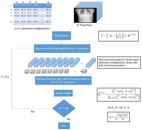
Figure 1.
The proposed hyper-parameter selection approach.
3.2. The Cross-Validation Approach
In order to compare the performance of the hyper-parameter selection approach using the Hedge algorithm, the cross-validation approach [30,31] is implemented. This approach is used to evaluate a predictive models by splitting the original data into training and testing sets. In one trial of the cross-validation approach, one projection is taken out from the available stack of projection data and is used as testing data. The remaining projections are used as training data. The reconstruction using the AwPCSD algorithm is implemented on the training set in parallel, using each one of the hyper-parameter configurations. The root-mean-square error (RMSE) refers to the sum of squares of the errors between the projected data associated with the reconstructed image for each hyper-parameter value, and the testing data. Then, the approach moves on to the next trial, where the next projection data is used as testing data. The same process is repeated again until the last available data is used as testing data. The average error of each hyper-parameter configuration is computed from the errors collected from all trials. At the end of the implementation, the best parameter configuration is the one with the lowest averaged error.
4. Numerical Studies
4.1. Experiments with Digital 4D Extended Cardiac-Torso (XCAT) Phantom
The first experiment to evaluate the proposed Hedge-based hyper-parameter selection approach is implemented by using the projection images simulated from a digital XCAT phantom [34]. Figure 2 displays the original XCAT phantom data used to simulate the input projection data using the GPU-accelerated forward operator available in the TIGRE toolbox [28]. The detector size is 512 × 512 pixels, with each pixel’s size of 0.8 mm. The image size is 128 × 128 × 128 voxels with the total size of 256 × 256 × 256 mm. Each image voxel’s size is 2 mm. The Poisson and Gaussian noise [35,36] has been added to the input projection data for a simulation of realistic noise. This is following the noise model presented in [18]. The maximum number of photon counts, which represents a white level for photon scattering, is specified as 60,000 from a 16 bit detector with some flat-field correction. The Gaussian noise is added to simulate electronic noise and obtained by a Gaussian random number generator with mean and standard deviation of 0 and 0.5, respectively.
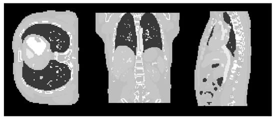
Figure 2.
The original XCATphantom data used to simulate input projection data for the experiments. Cross-sectional slices are shown in transverse, coronal and sagittal planes.
The experiments in this study were conducted by reconstructing images using an extremely low number of projection data, in order to demonstrate the performance of the proposed approach in a limited data CT reconstruction scenario. From the full set of projection data simulated for the entire 360° circle, 50 projection images are taken from this set equally sampled over 360, which represents ≈13% of the full projection data set. The results of image reconstruction from limited number of projection data using the FDK algorithm [9], as well as the AwPCSD algorithm with randomly chosen hyper-parameters () are shown in Figure 2 and Figure 3. It is clearly seen that the reconstructed image from the FDK algorithm suffers from notable artifacts due to the ill condition of the measured data, when the number of available projection data is limited. Although the reconstructed image from the AwPCSD with random hyper-parameters is slightly better than the FDK result, the quality of image is still far away from the exact phantom image. Hence, it is of the utmost importance to select the appropriate hyper-parameters values to obtain good reconstruction results.
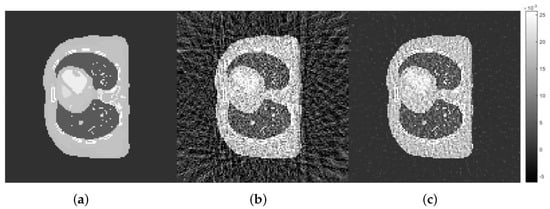
Figure 3.
Cross-sectional images from (a) the exact phantom image, (b) the FDK algorithm and (c) the AwPCSD algorithm with randomly chosen hyper-parameters ().
In our previously published work [21], the sensitivity of hyper-parameters for some common TV regularisation algorithms were analysed. The recommended values of some hyper-parameters were suggested following the conclusions from the experimental results. These values include = 1, = 0.99, to be set to the 90th percentile of the histogram of the reconstructed image from the OS-SART algorithm. These settings of the three hyper-parameters are followed in the experiments in this study. Therefore, there are two remaining hyper-parameters, and , that require a proper setting. The aim of the Hedging hyper-parameter selection approach proposed in this work is to select the best set of hyper-parameters from the user-defined ranges of two hyper-parameters, in combination with the three fixed-values hyper-parameters.
The proposed approach is aiming for any general users who do not have experience in CT reconstruction. Typically, the selection of hyper-parameters is often dependent on experts and can be problematic and time-consuming for general users to find the best hyper-parameters for TV regularised reconstruction algorithm with given data. With the proposed approach, the ranges of possible values can be specified and the approach will select the best set of hyper-parameter values from the user-defined ranges, once the approach finishes its implementation.
In this experiment, the values of all hyper-parameter configurations to be selected are shown in Table 1. The values for and can be defined by the user and were selected in this experiment to be rather broad, in order to cover all possible values of the hyper-parameters. There are 10 values of and 15 values of . The combination of these values leads to 150 different hyper-parameter configurations.

Table 1.
Values of each hyper-parameter configuration for this study.
As the total number of projection data (N) is 50, the initial starting image for the proposed approach is reconstructed using 25 projections (). Then, T is incremented by one, for the next iteration. In order to accelerate the process, the hyper-parameter configurations which produce probability of less than 10% of the highest probability are discarded before the approach moves on to the next iteration. The approach is iteratively implemented until T reaches N. The probability mass of all the parameter configurations at the end of the approach is shown in Figure 4.
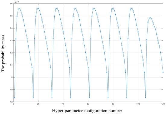
Figure 4.
The probability mass of all the hyper-parameter configurations after 25 iterations of the proposed Hedge-based algorithm (T = 25–50).
From a maximum a posteriori perspective, the best hyper-parameter configuration is the one with the highest probability. According to Figure 4, the highest probability is the configuration number 5 (, ). The lowest probability is the configuration number 16 (, ). Cross-sectional slices of the reconstructed images from the best and the worst hyper-parameter configurations are shown in Figure 5.
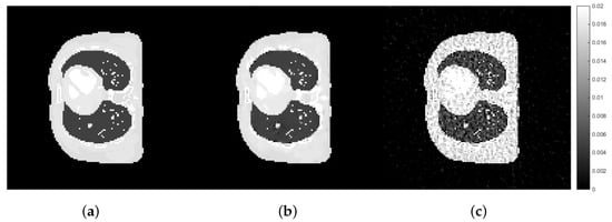
Figure 5.
Cross-sectional images from: (a) the exact phantom, (b) reconstruction with the best hyper-parameter configuration ( and ), and (c) reconstruction with the worst hyper-parameter configuration ( and ). The display window is [0–0.02].
It is seen in Figure 5 that the reconstructed image from the best configuration is better to preserve the important features of the image without being noisy compared to the result from the worst configuration.
4.2. Performance Evaluation
In order to evaluate the performance of the hyper-parameter selection approach using the Hedge method, the result is compared with the Cross-Validation method and the exact phantom image. Starting with the same initial ranges of the hyper-parameters as displayed in Table 1, the best hyper-parameter configurations, i.e., the values of two hyper-parameters ( and ), which have been found by the proposed Hedge-based approach and the Cross-Validation method are summarised in Table 2, together with the fixed values of the other 3 hyper-parameters.
Table 2.
Best hyper-parameter configurations have been found by the Hedge and the cross-validation algorithms.
It is worth mentioning here that the value of = 0 for the Hedge-based and Cross-Validation approaches does not mean that the approaches were able to achieve no error between the predicted and observed projection data. In this case, what happened was that the approaches aimed to reach the zero error point, when the hyper-parameter configuration under study contains = 0, but was forced to stop due to the maximum number of iterations being reached. Thus, the hyper-parameter configurations which contain were evaluated based on this attempt, in combination with the performance as affected by the other hyper-parameters.
In order to compare the results visually, the cross-sectional slices of the reconstructed images from the AwPCSD algorithm using best hyper-parameter configurations obtained using the proposed Hedge-based and Cross-Validation approaches are shown in Figure 6, as well as the one-dimensional profile plots along one arbitrary row of the reconstructed images in Figure 7. The results are compared with the exact phantom image as a reference image.
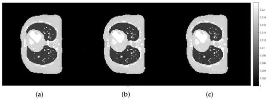
Figure 6.
Cross-sectional images from: (a) the exact phantom image, (b,c) are reconstructed images using the AwPCSD algorithm with best hyper-parameters from Cross-Validation and Hedge-based approaches, respectively.
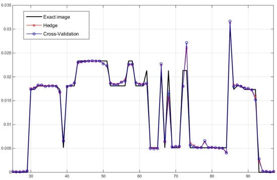
Figure 7.
One dimensional profile plots along pixel numbers 25 to 97 of the reconstructed images from two hyper-parameter selection methods along one arbitrary row of the images, in comparison with the exact image.
From visual inspection, the reconstruction results from the best hyper-parameters found by two approaches are very similar to each other. They are also relatively close to the exact phantom image, as confirmed by the one-dimensional profile plots in Figure 7. This means that the two approaches are able to identify the hyper-parameters which make the AwPCSD algorithm work efficiently and able to recover important features of the images. Comparing the results from two approaches, there are no important differences that could be visually observed. In order to quantify the differences between the results, the relative 2-norm and the Universal Quality Index (UQI) [37,38] are computed to explore the performance of the approaches for detailed structure preservation using the following equations:
where and denote voxel intensity of reconstructed image and reference image, respectively, m is the voxel index, Q is number of voxels, , and are covariance, variance and mean of intensities, respectively. The UQI is an image quality metric which is used to evaluate the degree of similarity between the reconstructed and reference images. The value ranges from zero to one, where a value closer to one suggests better similarity to the reference image.
Table 3 displays the relative errors, UQI values and the computational time taken to implement the hyper-parameter selection for the two approaches. The computational time is measured using the same computer (Intel Core i7-4930K CPU @3.40GHz with 32 GB RAM and GPU: NVDIA GeForce GT 610).
Table 3.
Relative errors, UQI and computational time of image reconstruction results from two hyper-parameter selection approaches. (Boldface numbers indicate the best result).
Quantitatively, the result from the Hedge-based approach is slightly better than the Cross-Validation approach with lower relative error and higher UQI. Comparing the computational time for each approach, the Cross-Validation approach took ≈ 47 h, whereas the Hedge-based approach took ≈ 16 h. It is understandable that the computational time for the Cross-Validation approach is much longer than for the Hedge-based approach since the Cross-Validation approach alternately uses each projection image as testing data and does so until the entire stack of projection data is used. The Hedge-based approach only starts its implementation from a pre-specified number of preliminary projections, which was specified as half of the available projection data () in the first experiment. The point of comparing the Hedge-based approach with the Cross-Validation approach is to prove the potential of the Hedge-based approach that; by computing the loss from the prediction and update the probability of each expert, the Hedge-based approach can drastically save computational time with quantitatively better result.
However, the computational time of ≈ 16 h of the Hedge-based approach in the first experiment is still quite long and requires further improvement. Such improvements can be made by focusing on two factors: the threshold to discard the hyper-parameter configurations from one iteration to the next iteration and the pre-specified number of preliminary projections (T). From trial-and-error, the improvement to the Hedge-based approach can be made by discarding the hyper-parameter configurations which produce a probability of less than 5% of the highest probability before proceeding to the next iteration and specifying . By doing these, the approach starts with a better quality of the preliminary image (based on 40 projections), but will only be implemented for 10 iterations (from to 50). In addition, the algorithm only allows hyper-parameter configurations with the top 5% probability passing through to the next iteration. The experiment with the new settings was conducted with the same XCAT phantom data as in the previous experiment. Upon completion of the implementation, the proposed approach with the new settings returned the same set of the best hyper-parameters () as that of the first experiment with computational time being ≈7 h. The computational time of the new settings is drastically reduced from the first experiment, approximately 8 h shorter. Thus, it can be concluded that the best setting to implement the proposed Hedge-based hyper-parameter selection approach is to specify and 5% from the highest probability as a threshold to discard the hyper-parameter configurations for the next iteration. These settings also yield the hyper-parameters with good reconstruction with much reduced computational time. Cross-sectional images of the AwPCSD algorithm with the best and worst hyper-parameters as found from the proposed approach with new settings are shown in Figure 8.
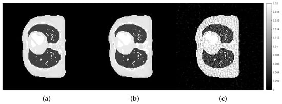
Figure 8.
Cross-sectional slices of (a) the exact phantom, (b,c) are the reconstructed images from the best ( and ) and worst ( and ) hyper-parameters found from the proposed approach with new settings ( and 5% threshold), respectively. The display window is [0–0.02].
4.3. Experiments with Different Datasets
For the next part of the study, the best set of hyper-parameters obtained from the previous experiment are applied to the reconstruction of different datasets with the same context, i.e., similar assumption about the x-ray measurements and materials/tissues. The aim is to observe whether the best hyper-parameters from the implementation of the proposed Hedge-based approach using one set of data can be readily applied to different datasets. For this purpose, we produced two new imaging data using also the digital XCAT phantom, but with different anatomical and motion parameters as shown in Table 4. The two datasets, male and female phantoms, are generated to represent the cases of different patients with different genders, as well as anatomical structures of the bodies. The parameters were specified randomly, aiming to generate as many differences as possible between the two datasets. The projection data were generated in the same way as in the first dataset. For the male phantom, the detector size is 512 × 512 pixels, with each pixel’s size of 0.8 mm. The image size is 128 × 128 × 70 voxels with the total size of 256 × 256 × 140 mm and image voxel’s size is 2 mm. For the female phantom, the detector size is similar to that of the male phantom. The image size is 128 × 128 × 48 voxels with the total size of mm and image voxel’s size is 2 mm. The experiments with these two datasets were also conducted using 50 projection images, equally sampled over 360. Cross-sectional slices of the two phantoms are shown in Figure 9.
Table 4.
The details of anatomical and motion parameters for male and female phantoms.
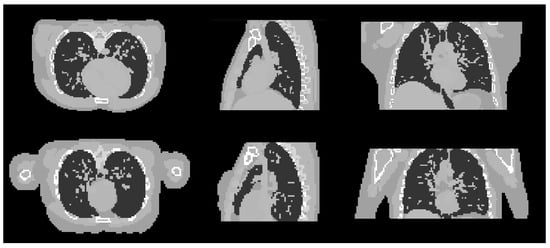
Figure 9.
Cross sectional slices of the male (top row) and female (bottom row) phantoms in the three axes.
The reconstruction using the AwPCSD algorithm with the best set of hyper-parameters from the training data set ( and = the 90t h percentile of the histogram of the reconstructed image from the OS-SART algorithm which are 0.0589 and 0.0748 for male and female datasets, respectively) was implemented with the male and female datasets. In addition, the AwPCSD algorithm using random hyper-parameters ( and /male, /female) was also implemented for comparison, as well as the exact phantom image. Cross-sectional images of these three cases are shown in Figure 10 and Figure 11, for male and female datasets, respectively.
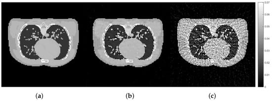
Figure 10.
The reconstruction results of the experiment with second dataset: male phantom: (a) exact male phantom image, (b) with the best hyper-parameters using the proposed Hedge-based approach with the first dataset (), (c) with random hyper-parameters ().
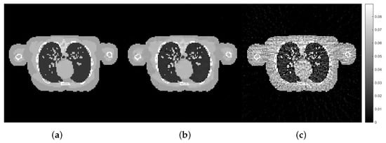
Figure 11.
The reconstruction results of the experiment with third dataset: female phantom: (a) exact female phantom image, (b) with the best hyper-parameters using the proposed Hedge-based approach with the first dataset (), (c) with random hyper-parameters ().
Figure 10 and Figure 11 show that the best hyper-parameters from the implementation of the proposed approach using one dataset can be applied for the reconstruction for different datasets and the images obtained via this approach are closer to the exact phantom image than the reconstruction obtained with random hyper-parameters. Depending on the task, the reconstructed images using the best hyper-parameters obtained from the training dataset may prove useful for a particular imaging application. The quality of the reconstructed image can be improved further by fine-tuning the set of hyper-parameters. It is very promising from the results that the set of hyper-parameters obtained from the training using the proposed Hedge algorithm can be readily applied to different datasets within a similar imaging context.
4.4. Experiments with Real Data
In previous section, discussion was focused on a medical phantom. In this final experimental section, we provide a case study using an industrial reference sample. The sample is designed by the National Physical Laboratory, United Kingdom. The reference sample is formed by standard geometries, including cylinders and cuboids. Both external and internal features are considered, which represent the most popular geometries used in engineering design. Different to medical phantom, the industrial reference sample is single material with clear boundary.
For industrial X-ray computed tomography, the quality of scan is an important factor. For a detector with 2000 × 2000, a complete scan requires 3142 projection images to ensure all pixels are covered in the scans from each rotation. However, with exposure time of 1 frame per second, one complete scan requires 52 min. This process is time consuming when there are significant number of samples to be measured. In order to reduce scan time, in the recent European Metrology Programme for Innovation and Research (EMPIR) project Advanced Computed Tomography for dimensional. and surface measurements in industry (AdvanCT), we have considered fast scan capability with less projection images. (Figure 12).
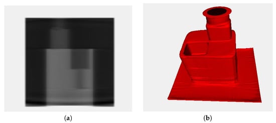
Figure 12.
(a) One projection of the original shape. (b) Reconstruction of a 3D shape.
5. Conclusions
XCT reconstruction from limited numbers of projection data is a challenging problem. The hyper-parameters in TV-penalised algorithms play an important role to balance the effects between the steps of data-consistency and positivity constraints and TV minimisation. Changing the values of hyper-parameters can drastically change the quality of the reconstructed image. Often, the hyper-parameters are calibrated by an expert. This work proposed the hyper-parameter selection approach for TV-penalised algorithm by combining the Hedge method of Freud and Shapire with the AwPCSD reconstruction algorithm. The Hedge algorithm is often analysed in terms of the distance to the optimal cumulated incurred by the best hyper-parameter configuration, as a function of the number of data observed so far, a criterion which is not rigorously equivalent to finding the best configuration based on visual reconstruction assessment. This makes the TV-penalised algorithms, specifically the AwPCSD, more generalised to be implemented by a general user.
The results showed that the proposed approach was able to select the best performance hyper-parameters from the user-defined values. The reconstructed image was compared with the Cross-Validation approach, which was considered as a straightforward approach to evaluate predictive model by splitting the original data into training and testing sets. The results from the Hedge and Cross-Validation approaches were visually indistinguishable and also very close to the exact phantom image. Quantitatively, the reconstructed image from the proposed approach was better than that of the Cross-Validation approach as measured by relative errors and the UQI metric. The computational time for the training using the proposed approach in the improved setting was hours, which is considerably shorter than for the Cross-Validation approach. The results with the other two datasets of the same imaging context but different anatomical and motion parameters showed that the best set of hyper-parameters derived from the training data also produced a good quality reconstructed image.
The main conclusion of this paper is that the proposed hyper-parameter approach using Hedge method provides a systematic way of choosing the hyper-parameters for the TV-regularised algorithm. Within the proposed framework, users can define a relevant range for the comparison of possible hyper-parameters configurations. Either the best performing hyper-parameters will be selected by the proposed method in the interior of the domain, or the selected hyperparameter values will lie on the boundary of the prescribed search domain, in which case the non-expert user will be able to relaunch the search within a larger domain in order to ensure that a relevant domain is explored. Numerical studies also showed the potential of readily applying the best hyper-parameters from the training dataset to other different datasets, which can save much time to avoid re-calibrating the hyper-parameters.
Author Contributions
Methodology, S.C.; Project administration, W.S.; Software, M.L.; Supervision, S.C. and W.S.; Validation, M.L.; Writing—original draft, M.L.; Writing—review & editing, W.S. and M.S. All authors have read and agreed to the published version of the manuscript.
Funding
This work was funded by the UK Government’s Department for Business, Energy and Industrial Strategy (BEIS) through the UK’s National Measurement System programmes. This project also has received funding from the EMPIR programme co-financed by the Participating States and from the European Union’s Horizon 2020 research and innovation programme.
Conflicts of Interest
The authors declare no conflict of interest.
References
- Candès, E.J.; Romberg, J.; Tao, T. Robust uncertainty principles: Exact signal reconstruction from highly incomplete frequency information. IEEE Trans. Inf. Theory 2006, 52, 489–509. [Google Scholar] [CrossRef]
- Donoho, D.L. Compressed sensing. IEEE Trans. Inf. Theory 2006, 52, 1289–1306. [Google Scholar] [CrossRef]
- Candès, E.J. Compressive sampling. In Proceedings of the International Congress of Mathematicians, Madrid, Spain, 22–30 August 2006; Volume 3, pp. 1433–1452. [Google Scholar]
- Candès, E.J.; Wakin, M.B. An introduction to compressive sampling. IEEE Signal Process. Mag. 2008, 25, 21–30. [Google Scholar] [CrossRef]
- Chrétien, S.; Darses, S. Sparse recovery with unknown variance: a LASSO-type approach. IEEE Trans. Inf. Theory 2014, 60, 3970–3988. [Google Scholar] [CrossRef]
- Bredies, K.; Kunisch, K.; Pock, T. Total generalized variation. SIAM J. Imaging Sci. 2010, 3, 492–526. [Google Scholar] [CrossRef]
- Goldstein, T.; Osher, S. The split Bregman method for L1-regularized problems. SIAM J. Imaging Sci. 2009, 2, 323–343. [Google Scholar] [CrossRef]
- Chambolle, A. An algorithm for total variation minimization and applications. J. Math. Imaging vis. 2004, 20, 89–97. [Google Scholar]
- Feldkamp, L.; Davis, L.; Kress, J. Practical cone-beam algorithm. JOSA A 1984, 1, 612–619. [Google Scholar] [CrossRef]
- Rudin, L.I.; Osher, S.; Fatemi, E. Nonlinear total variation based noise removal algorithms. Phys. D Nonlinear Phenom. 1992, 60, 259–268. [Google Scholar] [CrossRef]
- Sidky, E.Y.; Kao, C.M.; Pan, X. Accurate image reconstruction from few-views and limited-angle data in divergent-beam CT. J. X-ray Sci. Technol. 2006, 14, 119–139. [Google Scholar]
- Sidky, E.Y.; Pan, X. Image reconstruction in circular cone-beam computed tomography by constrained, total-variation minimization. Phys. Med. Biol. 2008, 53, 4777. [Google Scholar] [CrossRef] [PubMed]
- Liu, L.; Yin, Z.; Ma, X. Nonparametric optimization of constrained total variation for tomography reconstruction. Comput. Biol. Med. 2013, 43, 2163–2176. [Google Scholar] [CrossRef] [PubMed]
- Lu, X.; Sun, Y.; Yuan, Y. Optimization for limited angle tomography in medical image processing. Pattern Recognit. 2011, 44, 2427–2435. [Google Scholar] [CrossRef]
- Tian, Z.; Jia, X.; Yuan, K.; Pan, T.; Jiang, S.B. Low-dose CT reconstruction via edge-preserving total variation regularization. Phys. Med. Biol. 2011, 56, 5949. [Google Scholar] [CrossRef]
- Liu, L.; Lin, W.; Jin, M. Reconstruction of sparse-view X-ray computed tomography using adaptive iterative algorithms. Comput. Biol. Med. 2015, 56, 97–106. [Google Scholar] [CrossRef]
- Grudzien, K.; Romanowski, A.; Williams, R.A. Application of a Bayesian approach to the tomographic analysis of hopper flow. Part. Part. Syst. Charact. 2005, 22, 246–253. [Google Scholar] [CrossRef]
- Liu, Y.; Ma, J.; Fan, Y.; Liang, Z. Adaptive-weighted total variation minimization for sparse data toward low-dose x-ray computed tomography image reconstruction. Phys. Med. Biol. 2012, 57, 7923. [Google Scholar] [CrossRef]
- Perona, P.; Malik, J. Scale-space and edge detection using anisotropic diffusion. IEEE Trans. Pattern Anal. Mach. Intell. 1990, 12, 629–639. [Google Scholar] [CrossRef]
- Wang, J.; Li, T.; Liang, Z.; Xing, L. Dose reduction for kilovotage cone-beam computed tomography in radiation therapy. Phys. Med. Biol. 2008, 53, 2897. [Google Scholar] [CrossRef]
- Lohvithee, M.; Biguri, A.; Soleimani, M. Parameter selection in limited data cone-beam CT reconstruction using edge-preserving total variation algorithms. Phys. Med. Biol. 2017, 62, 9295. [Google Scholar] [CrossRef]
- Claesen, M.; De Moor, B. Hyperparameter search in machine learning. arXiv preprint 2015, arXiv:1502.02127. [Google Scholar]
- Padierna, L.C.; Carpio, M.; Rojas, A.; Puga, H.; Baltazar, R.; Fraire, H. Hyper-parameter tuning for support vector machines by estimation of distribution algorithms. In Nature-Inspired Design of Hybrid Intelligent Systems; Springer: New York, NY, USA, 2017; pp. 787–800. [Google Scholar]
- Lorenzo, P.R.; Nalepa, J.; Kawulok, M.; Ramos, L.S.; Pastor, J.R. Particle swarm optimization for hyper-parameter selection in deep neural networks. In Proceedings of the Genetic and Evolutionary Computation Conference, Berlin, Germany, 15–19 July 2017; pp. 481–488. [Google Scholar]
- Palar, P.S.; Zuhal, L.R.; Shimoyama, K. On the use of metaheuristics in hyperparameters optimization of gaussian processes. In Proceedings of the Genetic and Evolutionary Computation Conference Companion, Prague, Czech Republic, 13–17 July 2019; pp. 263–264. [Google Scholar]
- Freund, Y.; Schapire, R.E. A decision-theoretic generalization of on-line learning and an application to boosting. J. Comput. Syst. Sci. 1997, 55, 119–139. [Google Scholar] [CrossRef]
- Arora, S.; Hazan, E.; Kale, S. The Multiplicative Weights Update Method: a Meta-Algorithm and Applications. Theory Comput. 2012, 8, 121–164. [Google Scholar] [CrossRef]
- Biguri, A.; Dosanjh, M.; Hancock, S.; Soleimani, M. TIGRE: a MATLAB-GPU toolbox for CBCT image reconstruction. Biomed. Phys. Eng. Exp. 2016, 2, 055010. [Google Scholar] [CrossRef]
- Andersen, A.H.; Kak, A.C. Simultaneous algebraic reconstruction technique (SART): a superior implementation of the ART algorithm. Ultrason. Imaging 1984, 6, 81–94. [Google Scholar] [CrossRef]
- Arlot, S.; Celisse, A. A survey of cross-validation procedures for model selection. Stat. Surv. 2010, 4, 40–79. [Google Scholar] [CrossRef]
- Tibshirani, R. Regression shrinkage and selection via the lasso. J. R. Stat. Soc. Ser. B (Methodol.) 1996, 58, 267–288. [Google Scholar] [CrossRef]
- Chretien, S.; Gibberd, A.; Roy, S. Hedging hyperparameter selection for basis pursuit. arXiv preprint 2018, arXiv:1805.01870. [Google Scholar]
- Heidrich-Meisner, V.; Igel, C. Hoeffding and Bernstein races for selecting policies in evolutionary direct policy search. In Proceedings of the 26th Annual International Conference on Machine Learning, Montreal, QC, Canada, 14–18 June 2009; pp. 401–408. [Google Scholar]
- Segars, W.; Sturgeon, G.; Mendonca, S.; Grimes, J.; Tsui, B.M. 4D XCAT phantom for multimodality imaging research. Med. Phys. 2010, 37, 4902–4915. [Google Scholar] [CrossRef]
- Xu, J.; Tsui, B.M. Electronic noise modeling in statistical iterative reconstruction. IEEE Trans. Image Process. 2009, 18, 1228–1238. [Google Scholar]
- Ma, J.; Liang, Z.; Fan, Y.; Liu, Y.; Huang, J.; Chen, W.; Lu, H. Variance analysis of x-ray CT sinograms in the presence of electronic noise background. Med. Phys. 2012, 39, 4051–4065. [Google Scholar] [CrossRef] [PubMed]
- Wang, Z.; Bovik, A.C. A universal image quality index. IEEE Signal Process. Lett. 2002, 9, 81–84. [Google Scholar] [CrossRef]
- Zhang, H.; Ouyang, L.; Huang, J.; Ma, J.; Chen, W.; Wang, J. Few-view cone-beam CT reconstruction with deformed prior image. Med. Phys. 2014, 41, 121905. [Google Scholar] [CrossRef] [PubMed]


© 2020 by the authors. Licensee MDPI, Basel, Switzerland. This article is an open access article distributed under the terms and conditions of the Creative Commons Attribution (CC BY) license (http://creativecommons.org/licenses/by/4.0/).