Abstract
The Expectation-Maximization algorithm is adapted to the extended Kalman filter to multiple GNSS Precise Point Positioning (PPP), named EM-PPP. EM-PPP considers better the compatibility of multiple GNSS data processing and characteristics of receiver motion, targeting to calibrate the process noise matrix Qt and observation matrix Rt, having influence on PPP convergence time and precision, with other parameters. It is possibly a feasible way to estimate a large number of parameters to a certain extent for its simplicity and easy implementation. We also compare EM-algorithm with other methods like least-squares (co)variance component estimation (LS-VCE), maximum likelihood estimation (MLE), showing that EM-algorithm from restricted maximum likelihood (REML) will be identical to LS-VCE if certain weight matrix is chosen for LS-VCE. To assess the performance of the approach, daily observations from a network of 14 globally distributed International GNSS Service (IGS) multi-GNSS stations were processed using ionosphere-free combinations. The stations were assumed to be in kinematic motion with initial random walk noise of 1 mm every 30 s. The initial standard deviations for ionosphere-free code and carrier phase measurements are set to 3 m and 0.03 m, respectively, independent of the satellite elevation angle. It is shown that the calibrated Rt agrees well with observation residuals, reflecting effects of the accuracy of different satellite precise product and receiver-satellite geometry variations, and effectively resisting outliers. The calibrated Qt converges to its true value after about 50 iterations in our case. A kinematic test was also performed to derive 1 Hz GPS displacements, showing the RMSs and STDs w.r.t. real-time kinematic (RTK) are improved and the proper Qt is found out at the same time. According to our analysis despite the criticism that EM-PPP is very time-consuming because a large number of parameters are calculated and the first-order convergence of EM-algorithm, it is a numerically stable and simple approach to consider the temporal nature of state-space model of PPP, in particular when Qt and Rt are not known well, its performance without fixing ambiguities can even parallel to traditional PPP-RTK.
1. Introduction
Since Precise Point Positioning (PPP) emerged [1,2], people are primarily focusing on improving precise orbit and clock products, developing new algorithms to solve for ambiguities, to accelerate its convergence and expand its applications such as PPP-real-time-kinematic (PPP-RTK), triple frequency PPP [3], ionosphere-constraint PPP and low-cost receiver PPP [4,5,6,7,8,9,10].
Generally, PPP can be realized by the least-squares method (including sequential least-squares) or extended Kalman filter. The least-squares method is for static state estimation and thus does not reflect varying user dynamics. To work the same as Kalman filter, the process noise matrix is added to the gain matrix of the sequential least-squares method to adjust receiver clock behavior and atmospheric activity and so on, which is named as a sequential filter [2]. Hence, in the following paper, the authors will only consider the Kalman filter for PPP data processing.
Although both the process noise Qt and observation covariance matrix Rt are the key to Kalman filter, limited attention is paid to the fundamental problem for multi-GNSS PPP. Qt and Rt must be consistent with state dynamics and measurement accuracy, respectively. For example, if the value of Qt is too small, the estimated state will lose its minimum mean squared error property, and if the value of Qt is too large with respect to the correct one, the estimated state will oscillate around the true value. Moreover, because of ground deformation and specific surroundings, Qt should not be kept fixed to calculate the optimal estimates. In other words, Qt should evolve with time and a proper Qt will shorten the PPP convergence time. If Qt is improper, it may damage PPP convergence sometimes.
As for GNSS, Rt not only depends on the measurement accuracy, elevation of the satellite, orbit and clock error, atmospheric delay error, multipath, missing data, etc. but possibly deteriorate after a lapse of a period. What is more, the assumption, frequently used in geodesy, that different types of measurements have a fixed error ratio is not always true, because the ratio is closely linked to receivers and antenna types, and to the performance of satellite system itself. For example, while fusing multiple GNSS, the weight of measurements of GPS is intended to be higher, other GNSS systems to be lower. It is not easy to give a prior accurate ratio.
Generally, four methods are often applicable to calibrate Qt and Rt. The first one is based on the innovation property of the Kalman filter, in which a moving-window recursive way is used to identify Qt and Rt [11,12,13,14]. However, none of them can maintain the positive semi-definiteness of the estimated covariances. To solve this problem, Odelson developed the autocovariance least-squares method for estimating covariances using a lagged autocovariance function [15]. This kind of least-squares method depends on the user-defined autocovariance function.
The second scheme to recognize Qt and Rt is the multiple model adaptive estimation (MMAE) [13,16]. MMAE runs a bank of Kalman filter in parallel, every one of them is driven by its pair of Qt and Rt. The final Qt and Rt are thought of as the weighted sum of the estimates of individual Kalman filter.
In the third scheme, M-estimator is introduced into an adaptive Kalman filter to increase its resistance to outliers, where an adaptive factor to state error covariance matrix is constructed [17,18]. Yet, choosing a value for is still very challenging. An improper will result in biased results.
Another attractive scheme is the least-squares variance component estimation (LS-VCE) [19], which is based on least-squares principles. Similar to restricted maximum likelihood (REML), LS-VCE does not use observations directly but combine observations to exclude any fixed effects. However, LS-VCE needs to define the weight matrix on the user‘s own and increase its complexity.
In this contribution, a machine learning algorithm, the Expectation-Maximization (EM) algorithm, is developed to the extended Kalman filter to estimate PPP states, , together with a large number of Qt and Rt. The EM-algorithm, which can be classified as the first scheme, works in an iterative procedure to locate maximum likelihood estimates of parameters. Its iteration consists of two steps: Expectation and Maximization. In the Expectation step, a function for the expectation of the log-likelihood is computed using the estimates of the current parameters. In the Maximization step, estimates of parameters are updated by maximizing the expected log likelihood function.
On the one hand, the main drawback of the EM-algorithm is that it converges slowly and needs heavy computation. Here the convergence refers to finding maximum likelihood estimator of parameters, not the PPP convergence time. However, for example, its convergence can be accelerated using the Aitken method or conjugate method [20].
On the other hand, it is fairly simple, and has robust convergence and deals conveniently with problems having a lot of parameters. For such problems, it is often the only algorithm to a large extent [19]. It is also capable of finding Kalman parameters even if we have missing data. In addition, it can detect outliers by introducing small weights for large outliers and can even estimate the outliers [21]. In contrast, the outliers are not removed but automatically downweighed in our article, since outliers sometimes take some useful information.
The paper is organized as follows, after clarifying the importance to calibrate Qt and Rt, the EM algorithm is introduced in the first section. Next, the state space model of PPP is reviewed from a point of machine learning and the methodology to adapt the EM-algorithm for extended Kalman filter for PPP is explained theoretically in detail. Thirdly, we compare the EM-algorithm with other methods, the static and kinematic instances are also given to demonstrate EM-PPP performance to improve the accuracy and reliability of PPP. Finally, the results are analyzed and the conclusion is drawn.
2. State Space Model for PPP
The state-space model allows to process GNSS data in a uniformed form. It is characterized as two equations: the state equation, which comprises a series of vector , is the number of epochs), and the observation equation. The state cannot be observed directly, usually called hidden states, which is driven by hidden process noise. In this article the state-space model is described as the Kalman filter.
2.1. State Equation
The hidden state of multi-GNSS PPP Kalman filter involves five types of parameters: three components of receiver coordinates, receiver clock error, system time difference w.r.t. GPS, troposphere zenith wet delay and ambiguities. Using subscript to denote a specific time epoch, the state at time evolves from the state at ( according to:
where is the transition matrix and the state process noise, which is assumed to be drawn from a zero-mean multivariate normal distribution, with covariance: . Initial condition is assumed to be a Gaussian vector with the a priori information .
The state transition matrix and the process noise matrix in static mode is defined for the position block:
where , and are the random process noise in , and direction, respectively.
In addition to position parameters, the velocity parameters are also included in the state vector for our kinematic processing, whose system model for position and velocity block in the extended Kalman filter is given as:
The corresponding state vector is for position and velocity block. The process noise matrix is uniquely determined by and , which are named as acceleration variance.
2.2. Observation Equation
The observation equation, that we used, is the double frequency ionosphere-free combination for multi-GNSS [22]:
where subscript r indicates the receiver, superscript represents the satellites, superscript indicates GNSS constellation, following the convention of Rinex3.x (G: GPS, E: GALILEO, R: GLONASS and C: BEIDOU). and are the ionosphere-free combinations of code pseudo-range and phase observations (unit: m) respectively, which have already corrected satellite clock, the relativity effect, solid Earth tides, polar tides, ocean tides, phase wind up and a priori troposphere delay using troposphere model [23,24]. is the geometry distance between receiver and satellite, is receiver clock (unit: m), the superscript of implies that GPS time is selected as the reference time, is the system time difference in meters of system to GPS time. Specifically, for is zero. is troposphere mapping function and is troposphere zenith wet delay, is the wavelength of LC combination corresponding to system and is the LC ambiguity. and indicate other unmodeled errors or noise.
Equations (4) and (5) are nonlinear, the extended Kalman filter (EKF) can be used for nonlinear state estimation. For easy description, they are rewritten in a general form:
where is the observation vector, is the number of observations at epoch , , is the observation noise satisfying , is the observation noise covariance matrix at epoch .
2.3. Kalman Filter
Let denote all observations from epoch 1 to epoch , and represent the estimate of given observations , we have predicted state estimate and predicted covariance estimate:
After linearization of Equation (6) at predicted state ,
where . is called innovations or measurement residuals, then the Kalman filter is obtained:
where and are the updated Kalman estimate and the updated covariance estimate.
2.4. Kalman Smoothing
The Kalman smoother estimator could be obtained [25]:
where , is the number of epochs.
Kalman lag-one covariance holds with the starting condition
for
3. EM-PPP
The EM-algorithm is based on the innovation of the likelihood function to compute maximum likelihood estimation [25,26]. The likelihood function describes the probability of the observations, given a set of parameters. The parameters are found such that they maximize the likelihood function. The derivative of the likelihood function or log-likelihood is not always tractable. Therefore, iterative methods like Expectation-Maximization algorithms are very effective to find numerical solutions for the parameter estimates.
Denoting , . Y is thought of as incomplete data, and as complete data. Specifically for PPP, the log likelihood of the parameters of the state space model is approximately derived (ignoring constant):
Since the hidden states are unknown, only the expected value of the log likelihood conditioned on Y is accessible, as a result, the observation equation is expanded at smoother point .
The Expectation (E-step) of EM algorithm for PPP requires computing the expected log-likelihood at the iteration:
then the parameters are recalculated at the Maximization step (M-step):
The two steps are repeated until the converges.
The EM-PPP is terminated when the following convergence criterion is reached:
where is a small predefined amount and is equal to
A flowchart of our EM-PPP procedure is shown in Figure 1. In the initialization step, GNSS data preprocessing is performed including data integrity checking, cycle slips and outliers detection, phase center offset (PCO) and phase center variations (PCV) correction, synchronization of receiver clock using only code range measurements and initialization of parameters . It also initializes the hidden state , sharing of the same processing noise across the time step
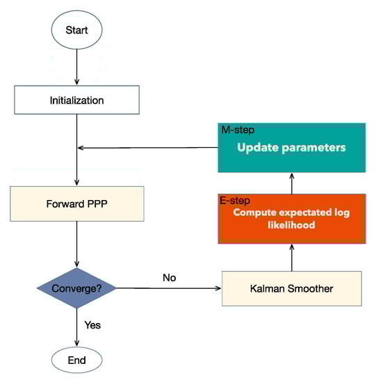
Figure 1.
Flowchart of the Expectation-Maximization (EM)-Precise Point Positioning (PPP) loop.
In the next step, the extended Kalman filter Equations (10)–(12) are implemented to compute a series of hidden states and their covariance. If the convergence condition Equation (20) is not satisfied, then Kalman smoothing is used to calculate smoothed state estimates and involved covariance matrix Equations (13)–(16), which is prepared for the E-step: calculation of the expected log likelihood function Equation (22). All parameters of are updated during the M-step and prepared for the next iteration Equation (27).
3.1. E-Step
Taking the expectation upon Equation (17) over conditional distribution of the latent given observed data, we find immediately:
where
Using Taylor series expression
where , and let , we get
3.2. M-Step
Similar to complete-data weighted maximum likelihood estimation, from the first differential of , the maximum likelihood estimators are updated as follows:
For simplicity, the initial covariance , and the measurement covariance are assumed to be a diagonal matrix:
where indicates the dimension of the hidden state vector at initial epoch and is the dimension of the observation vector at epoch
4. EM Compared to MLE and LS-VCE
In literature [19], a comprehensive comparison is demonstrated between different estimation principles such as LS-VCE, best linear unbiased estimator (BLUE), best invariant quadratic unbiased estimator (BIQUE), minimum norm quadratic unbiased estimator (MINQUE) and restricted maximum likelihood estimator (REML). As shown previously in Section 3.1, the EM algorithm may be thought of as maximum likelihood estimation (MLE), but which finds the ML estimator in an iterative way. EM can be realized based on REML as well. Therefore, an additional comparison between EM variance estimation and LS-VCE and MLE is adequate.
To make theoretical analysis easy and consistent, in the following we first introduce how to covert Kalman filter to least-squares. Then we directly give different (co)variance estimators according to their distribution assumptions and the reason why the EM-algorithm is preferable in our solution.
4.1. From Kalman Filter to Least Squares
The linear (extended) Kalman equation can be transformed into the least-squares function model, which allows the following EM algorithm to be compared with LS-VCE on the same function model and makes the theoretical analysis easy and convenient. To do so, the state Equation (1) and the observation Equation (6) are expanded at a priori value and organized as the function model:
with
where the a priori value is subtracted from the original state vector , leading to and , is the number of epochs. The matrix A is full column rank. The cofactor matrices , are assumed to be known and their weighted sum is assumed to be positive definite and are linearly independent, and the (co)variance components are unknown parameters. Matrix is the known part of the variance matrix [19].
4.2. Least-Squares EM
Similar to Section 3, we can calculate the non-constant part of the full log-likelihood function and then conditional expectation on the observation and , given the data and the iteration estimates of (co)variance components or :
where
M-step:
Maximizing the likelihood of the completed data based on Equation (29), the new estimates are calculated as
where , , is the Kronecker product and vec is -operator.
Equations (29) and (31) are the EM algorithm for ML estimation. If convergence is reached, set , otherwise increase by one and return to E-step.
4.3. MLE
Once the general structure of probability density function is known, MLE can be simply realized and therefore used widely. If a multivariate normal distribution is given, the (co)variance components takes form:
where , .
From Equations (31) and (32), we know that least-squares EM and MLE estimators share the same design matrix and weight matrix. Their difference is mainly caused by the pseudo observation and . for EM-algorithm includes the effects of both observation post-residuals and the accuracy of the estimates . In contrast, for MLE consider only the observation post-residuals. Therefore, MLE estimator is probably over-optimistic to EM.
However, if the REML principle is used to derive the EM-algorithm, the effect of is implicitly removed. Then, the EM-algorithm based on REML will be equivalent to the REML estimator.
4.4. LS-VCE
Another important problem is that the EM-algorithm and MLE do not take the loss of degrees of freedom from the estimation of into account. Borrowing the idea of REML, LS-VCE overcomes this problem based on ( independently error contrasts. Specifically, let
where is misclosure vector, is matrix satisfying , . Then LS-VCE estimator is obtained:
with , , is a user-defined weight matrix. If is set to , LS-VCE is the same as EM-algorithm based on REML.
LS-VCE is derived purely based on the least-squares method and we do not make any assumption on a probability density function (PDF). In contrast, EM-algorithm, MLE and REML are built upon a certain distribution, which explains why when applying LS-VCE, it is necessary for users to set weight matrix on their own.
4.5. Preference for Recursive EM
As discussed previously, the EM-algorithm can be implemented as either recursive form or batch form like MLE and LS-VCE. In our solution, we prefer the EM-algorithm based Kalman filter to other methods.
Recursive EM discriminates between the process noise and the observation noise. For GNSS, the process noise is usually different from observation noise. The process noise is directly connected to the geophysical phenomenon, which has not only linear but also non-linear variations, and suffers both time and spatial correlations [27,28,29]. As a result, it is relatively more difficult to estimate the process noise than the observation covariance matrix. Other batch methods mix the two types of stochastic processes with different behavior, which will bring us extra trouble.
Recursive EM can process data in not only post mode, but also in real-time mode. In both modes, data is processed epoch by epoch, allowing us to dynamically adjust the weight matrix, monitoring time-varying behavior and detecting abrupt motion.
5. Validation
5.1. Static PPP Scheme
A total of 14 IGS multi-GNSS stations are selected to assess the performance of EM-PPP (Figure 2). Those stations are evenly distributed on the Earth and track as many GNSS constellations as possible, covering not only the continent but also coastal and polar regions.
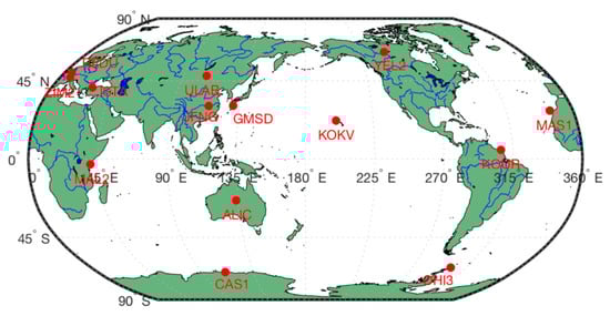
Figure 2.
Distribution of selected IGS multi-GNSS stations.
Daily GNSS measurements from those IGS stations observed during DOY 119 in 2017 are used in this study. The true coordinate benchmarks are from IGS weekly solutions. The final GFZ Beidou multi-GNSS (GBM) products of the satellite orbits and clocks are applied (ftp://cddis.gsfc.nasa.gov/pub/gps/products/mgex/). The used precise orbit correction has a sampling interval of 15 min while the precise clock has a sampling interval of 30 s, both generated at GFZ. For GPS, we aligned C1 to P1 using CODE differential code bias (DCB) product (ftp://ftp.aiub.unibe.ch/CODE/2017/). The frequency bands we used are L1 and L2 for GPS, G1 and G2 for Glonass, E1 and E5a for Galileo, B1 and B2 for BeiDou [9]. Receiver and satellite PCO and PCV were corrected using igs14.atx. solid Earth tides, pole tide and ocean tides are removed according to IERS Conventions 2010. For troposphere delay estimation, the zenith dry component of tropospheric delays was corrected with the a priori Niell model [24]. The zenith wet delay (ZWD) is estimated as an unknown parameter. Then, 24-h observation data sets with a sampling interval of 30 s were processed for all stations. The elevation cut-off was set to 6 degrees.
The initial guess of receiver coordinates is intentionally deviated by 100 m from IGS station solution. A priori standard deviation (std) of PC is set to 3 m, a priori std of LC to 0.03 m for pseudo-range combination (PC) and carrier phase combination (LC) combination, respectively.
The starting values for are shown in Table 1. Random walk noise process with a spectral density equal to 1.0 mm/ s is imposed on coordinates, which means a 1.0 mm disturbance very 30 s for IGS station in North, East and Up. It is not true in reality of course, but useful for test purposes. The receiver clock offset is supposed to be white noise. Zenith wet delay (ZWD) and inter-system bias (ISB) are modeled as random walk noise. Ambiguities can be considered as constant or random walk noise with very small spectral density.

Table 1.
Initial guess for static PPP: ZWD is the zenith wet delay of the troposphere, ISB is the system time difference with respect to GPS time.
If the maximum number of iteration is reached and EM-PPP does not converge, smaller spectral density should be assigned for X, Y and Z for the next cycle.
5.2. Kinematic PPP Scheme
Another kinematic dataset was used to further validate the performance of the EM-PPP. The data was collected at Wuhan, China, in November 14, 2013. The sampling interval is 1 Hz and the observed time span is about one hour. The final CODE precise satellite orbit and 5 s clock products are used to estimate the 1 Hz GPS displacements. The ambiguity-fixed double differenced real-time kinematic (RTK) solutions are adopted as the reference to assess the performance of kinematic EM-PPP solution.
The initial acceleration variance is assumed to be for position and velocity states (Table 2), which can be used to calculate the process noise matrix for position and velocity. The initial Qt for receiver clock is modeled as white noise and estimated epoch-wisely. ZWD and ambiguities are also modeled as random walk processes with initial spectral density 0.01 cm/ and 0.0 m/, respectively.
Table 2.
Initial guess for kinematic PPP: ZWD is zenith wet delay of troposphere.
6. Results and Discussion
6.1. Static EM-PPP Solution
It is found that EM-PPP usually converges after the iteration counter reaches 50. The positioning errors are shown in Table 3, including PPP results at 1st iteration with the biased stochastic model, and the results after 50 iterations of calibration to assess EM-PPP performance. EM-PPP convergence in our research means that the square root of 3D positioning errors of the last 20 consecutive epochs is less than 10 cm.
Table 3.
Statistics of EM-PPP absolute positioning errors (cm) with respect to IGS stations solution. All sites except YEL2 are processed using multiple GNSS observations. YEL2 is processed using only GPS data to verify the algorithm for single GNSS constellation. The ambiguities are not fixed.
Table 3 indicates that when the biased Qt and Rt are fed in the beginning, PPP 3D errors are up to decimeters for a few stations. Horizontal errors are often greater than vertical errors, which is not consistent with the property of GNSS, because of inappropriate process noise matrix and measurement noise covariance matrix. After 50 iterations, the position errors are reduced to within 1 cm in North, East and Up direction on average using our EM-PPP algorithm. The mean 3D error is reduced to 1.77 cm without fixing ambiguities. The overall decrease percentage on average is 66.91%, 66.16%, 71.60% in North, East and Up direction, respectively, 69.95% for 3D errors.
To see what happened to the process noise and the observation covariance matrix before and after calibration, an example of JFNG station located in China is illustrated.
The residuals for PC and the corresponding formal errors are shown in Figure 3. The residuals for LC and the corresponding formal errors against satellite elevation angles after calibration are shown in Figure 4. To be clear, PC and LC residuals for BeiDou are plotted separately from those for GPS, Glonass and Galileo.
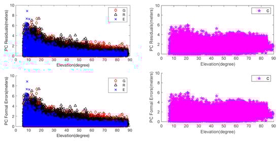
Figure 3.
EM-PPP absolute pseudo-range combination (PC) residuals and formal errors of JFNG station at 50th iteration: Left two pictures are the PC residuals and their formal errors (square root of observation matrix ) of GPS, Glonass and Galileo, respectively. Similarly, the right two pictures show the PC residuals and formal errors of BeiDou.
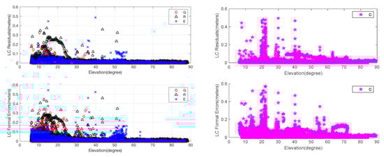
Figure 4.
EM-PPP carrier phase combination (LC) residuals and formal errors of JFNG station at 50th iteration: Left two pictures are the LC residuals and formal errors (square root of the observation covariance matrix) for GPS, Glonass and Galileo, respectively. Similarly, the right two pictures show the LC residuals and formal errors for BeiDou.
The results allow us to examine the relationship between and the residuals. It is clearly shown that formal errors of are changed from 3 m to vary about between 0 and 10 m for PC, and from 0.03 m to vary about between 0 and 0.6 m for LC. The big outliers of LC are due to the non-convergence at the initial epoch and EM-PPP does not fully converge at some epochs. Although variations, similar to the residuals-varying pattern, are dependent on the satellite elevation angle, LC formal error of BeiDou at the elevation of about 20 degrees is greater than the lower degree formal error (refer to the bottom right picture in Figure 4). Clearly, it is not advisable to choose observation weight only according to the satellite elevation angle. Another example is station ISTA, where Glonass Rt for PC at satellite elevation higher than 50 degrees is almost as great as lower degree errors (not plotted here). In addition, random or systematic outliers are downweighed accordingly for both PC and LC.
It can also be observed that BeiDou PC residuals peak are almost 6 m, worse than GPS, Glonass and Galileo at JFNG. In fact, the biggest error source comes from GEO C05 and IGSO C06, C07 and C08, probably due to their poor orbit accuracy and clock offset, because the residuals of those satellites show less independence of satellite elevation angle. is different among GPS, Glonass and Galileo.
Thus not only reflects the accuracy of measurement type itself, elevation-dependent, characteristics of GNSS constellation, but also the quality of GNSS satellite orbit and clock products, and should be adjusted dynamically. Consequently, EM-PPP is effective to calibrate automatically and suppress outliers.
In general, can be adjusted to its correct value, which is zero in our case, after less than ten iterations, as shown in Figure 5. The initial square root of in North, East and Up directions are 0.001 m/ s. Qt becomes zero at the sixth iteration in all three components and position solution at the last epoch varies little.
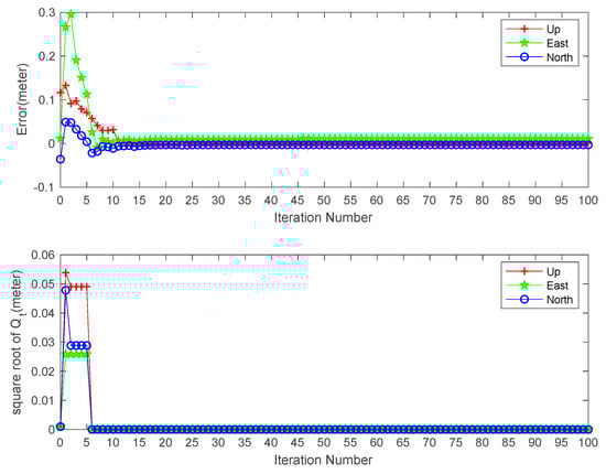
Figure 5.
Effects of EM-PPP iteration number on the position errors (top) and variations of the square root of at last epoch on station JFNG.
It has to be pointed out that EM-PPP suffers local extrema problems like other alternative methods. It is not an algorithm to locate the global maxima, therefore EM-PPP is sensitive to initial guesses. To escape from this local extrema trap, several sets of initialization schemes can be used, and select the best one selected as the final result.
6.2. Kinematic EM-PPP Solution
Figure 6 is the tracking route recovered by the EM-PPP at the 500th iteration. The relative log-likelihood versus iterations is plotted in Figure 7, where the results at the first iteration correspond to the solution to the traditional PPP (TPPP). The relative log likelihood decreases gradually from 1.0 to 8.665 × 10⁻⁷ and forms a concave curve. The less the relative log-likelihood, the less perturbative the EM-PPP solution becomes with respect to the RTK solution. As the iterative number grows to about 150, the EM-PPP solution converges nearly completely.
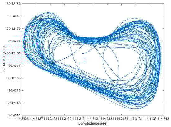
Figure 6.
Driving route of moving vehicle in Wuhan, China on 14 November 2013.
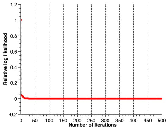
Figure 7.
Relative log-likelihood of two consecutive iterations.
Illustrated in Figure 8 are the positioning errors of the traditional PPP solution and EM-PPP solution at the 500th iteration with respect to the reference coordinates in the Up, East and North directions. It is observed that EM-PPP solutions are much more stable in all directions when compared to TPPP solutions. The TPPP solution in the East changes wobbly in comparison to the North and Up due to greater acceleration in the East (Figure 9), which leads to a larger bias in the East.
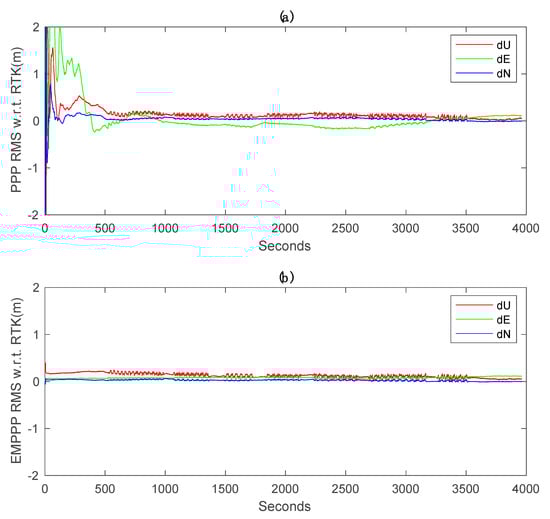
Figure 8.
GPS-only kinematic positioning errors with respect to real-time kinematic (RTK): (a) traditional PPP errors, (b) EM-PPP positioning errors at the 500th iteration. Traditional PPP and EM-PPP share the same initial conditions.
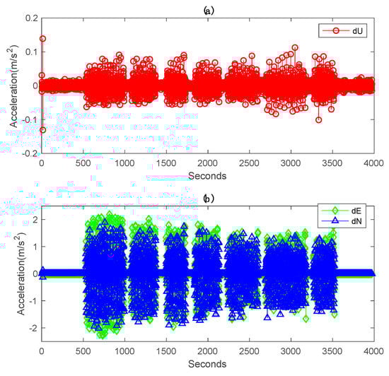
Figure 9.
Acceleration time series derived from second-order differencing RTK position time series in Up, East and North: (a) acceleration in Up. (b) Accelerations in the East and North.
In fact, the position and velocity (PV) model of our kinematic state equation is assumed to be a constant velocity model, which means the acceleration is zero. However, the realistic acceleration of the vehicle is no zero, which results in systematic bias and unstable solution.
Figure 10 and Figure 11 describe the EM-PPP RMSs and STDs with respect to RTK against the number of iterations, respectively. Obviously, after about 40 iterations, RMSs in Up and North are decreasing and the solutions are improved in those two directions. In contrast to Up and North direction, in the East direction it presents a decrease from 9.7 cm falling to 7.6 cm and then increases up to 8.5 cm for the RMS. However, the combined effects of all three directions get decreasingly 3D RMS, proving that EM-PPP does improve the positioning accuracy in the kinematic mode in our case, and apparently converges with increasing iterations, consistent with the EM theory, though there is a little disturbance because of the existing system bias and outliers of pseudo-range. It can be imagined that a better result can be expected if acceleration observations are also observed.
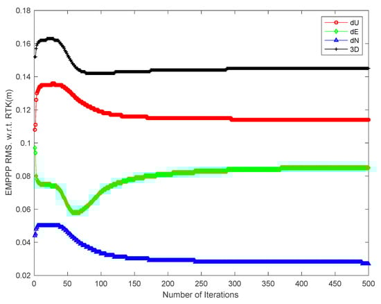
Figure 10.
EM-PPP RMSs w.r.t. RTK solution in Up, East and North (unit: m).
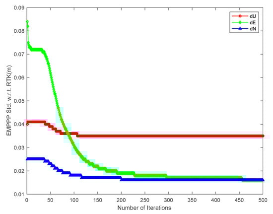
Figure 11.
EM-PPP STDs w.r.t. RTK solution in Up, East and North (unit: m).
As for STDs with respect to RTK, they are consistently increasing in all three directions when EM-PPP continues its iteration. The STDs decrease from 4.0 cm, 8.4 cm and 2.5 cm to 3.5 cm, 1.6 cm and 1.6 cm in Up, East and North components, respectively. In other words, the STDs are improved by 12.5%, 80.9% and 36.0% in Up, East and North, accordingly.
Given Figure 12 is the estimates of geodetic coordinates B, L and H, and their estimates of the square root of Qt after the 500th iteration. It is noted that the coordinates simultaneously stay stable or alternatively change sharply in all three directions, telling that the moving patterns of the vehicle switch between static and kinematic status from time to time. Theoretically, the process Qt should change between zero and positive values. Obviously, the estimates of the square root Qt, displayed in Figure 12b–f agree well with variations of coordinates. Time-varying Qt is identified, which takes the concrete dynamic mode into consideration.
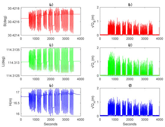
Figure 12.
EM-PPP estimates of the Geodetic coordinates B, L, H and their correspondingly calibrated Qt after the 500th iteration: (a) Latitude estimates B (degree). (b) The square root of Qt of B (m). (c) Longitude estimates L (degree). (d) The square root of Qt of L (m). (e) Height estimates H (m). (f) The square root of Qt of H (m).
If much smaller initial acceleration variances are given, for example rather than for position and velocity states, it can be shown that our algorithm can still recover the process noise matrix as well and makes no difference. As a result, the user can choose values for Qt randomly to a large extent.
7. Conclusions
A machine learning algorithm, EM algorithm, is adapted particularly to the extended Kalman filter to calibrate the process noise matrix and observation covariance noise matrix for PPP. The main advantage of EM-PPP is in fact that it is straightforward, simple, (locally) optimal and able to estimate large amounts of parameters and thus competent in calibrating the time-varying process noise and observation covariance for PPP state-space model, though its execution is time-consuming. The basic framework of EM-PPP is not limited to multi-PPP and can be applied to other fields of geodesy.
The whole procedure of EM-PPP is comprised of three parts: initialization, feedforward and backpropagation. In the beginning, the GNSS preprocess is performed to check the availability of the required data and mainly recognize cycle slips. Next, the whole process iterates between the estimation of hidden state and expectation and maximization.
The EM-algorithm is then compared with MLE and LS-VCE methods. We choose the recursive algorithm because it is superior to separate the process noise and observation variance, and to monitor time-varying behavior.
The approach was verified by selecting a global distribution of 14 IGS multi-GNSS station without fixing ambiguities. Based on the presented results, it concluded that EM-PPP is well suited for dynamically determining the time-varying process noise and observation noise. The calibrated observation variance matches the observation residuals from low satellite elevation angle to high satellite elevation angle. It resists orbit and clock errors and outliers through downweighing abnormal observations at different epochs, which is an alternative reasonable solution in contrast to the popular way that assigns weight according to the satellite elevation angle. People do not need to worry about separating observations into different categories carefully based on different GNSS constellations to estimate variance components like variance component estimation (VCE).
The spectral density of the assumed kinematic IGS station with 1 mm disturbance every 30 s in North, East and Up direction was estimated to be zero, implying that stations are static, which is consistent with reality.
An additional kinematic test was also implemented and reasonable values of Qt are found when biased initial Qt guess was given. The position errors are reduced in Up, East and North direction, respectively, w.r.t. RTK. In particular the STDs with respect to RTK are improved by 12.5%, 80.9% and 36.0% in Up, East and North, further showing that EM-PPP is also beneficial to kinematic PPP.
It has been confirmed that the EM-PPP is competitive for the calibration of the PPP stochastic model dynamically. The main drawback of this approach is that it converges slowly due to its first-order convergence. In the future, online EM-PPP may be derived to process GNSS data in real-time to overcome this problem if a large number of observations are available.
Author Contributions
X.Z. conceived and designed the algorithm; P.L. provided the kinematic GNSS data and helped validate the algorithm; M.G. supervised the whole procedure, and continuously discussed and analyzed the results and gave constructive suggestions; R.T. and X.L. participated in the experimental investigation; H.S. helped edit and revise the paper. All authors have read and agreed to the published version of the manuscript.
Funding
This research is funded by the China Scholarship Council (CSC).
Acknowledgments
X.Z. is financially supported by the China Scholarship Council (CSC) for his study at the German Research Centre for Geosciences (GFZ). We thank the IGS and GFZ for providing GNSS observations, DCBs, precise orbit, and clock products. Our research is also partly supported by the Chinese Academy of Sciences (CAS) program of “Light of West China” (Grant No. 29Y607YR000103), Chinese Academy of Sciences, Russia and Ukraine and other countries of special funds for scientific and technological cooperation (Grant No. 2BY711HZ000101). This work is also partly supported by the National Natural Science Foundation of China (Grant No: 41674034, 41974032, 11903040), the Chinese Academy of Sciences (CAS) programs of “Pioneer Hundred Talents” (Grant No: Y923YC1701), and the Chinese Academy of Sciences (CAS) program of “Western Youth Scholar” (Grant No: Y712YR4701, Y916YRa701), as well as “The Frontier Science Research Project” (Grant No: QYZDB-SSW-DQC028). We also thank the reviewers for their careful review.
Conflicts of Interest
The authors declare no conflict of interest.
References
- Zumberge, J.F.; Heflin, M.B.; Jefferson, D.C.; Watkins, M.M.; Webb, F.H. Precise point positioning for the efficient and robust analysis of GPS data from large networks. J. Geophys. Res. Solid Earth 1997, 102, 5005–5017. [Google Scholar] [CrossRef]
- Kouba, J.; Héroux, P. Precise point positioning using IGS orbit and clock products. GPS Solut. 2001, 5, 12–28. [Google Scholar] [CrossRef]
- Li, P.; Zhang, X.; Ge, M.; Schuh, H. Three-frequency BDS precise point positioning ambiguity resolution based on raw observables. J. Geod. 2018, 92, 1357–1369. [Google Scholar] [CrossRef]
- Ge, M.; Gendt, G.; Rothacher, M.A.; Shi, C.; Liu, J. Resolution of GPS carrier-phase ambiguities in precise point positioning (PPP) with daily observations. J. Geod. 2008, 82, 389–399. [Google Scholar] [CrossRef]
- Laurichesse, D.; Mercier, F.; Berthias, J.; Broca, P.; Cerri, L. Integer ambiguity resolution on undifferenced GPS phase measurements and its application to PPP and satellite precise orbit determination. Navigation 2009, 56, 135–149. [Google Scholar] [CrossRef]
- Collins, P.; Bisnath, S.; Lahaye, F.; Héroux, P. Undifferenced GPS ambiguity resolution using the decoupled clock model and ambiguity datum fixing. Navigation 2010, 57, 123–135. [Google Scholar] [CrossRef]
- Seepersad, G.; Bisnath, S. Reduction of PPP convergence period through pseudorange multipath and noise mitigation. GPS Solut. 2015, 19, 369–379. [Google Scholar] [CrossRef]
- Banville, S.; Collins, P.; Zhang, W.; Langley, R. Global and regional ionospheric corrections for faster PPP convergence. Navigation 2014, 61, 115–124. [Google Scholar] [CrossRef]
- Li, P.; Zhang, X.; Guo, F. Ambiguity resolved precise point positioning with GPS and BeiDou. J. Geod. 2017, 91, 25–40. [Google Scholar]
- Li, P.; Zhang, X.; Ren, X.; Zuo, X.; Pan, Y. Generating GPS satellite fractional cycle bias for ambiguity-fixed precise point positioning. GPS Solut. 2016, 20, 771–782. [Google Scholar] [CrossRef]
- Mehra, R. On the identification of variances and adaptive Kalman filtering. IEEE Trans. Autom. Control 1970, 15, 175–184. [Google Scholar] [CrossRef]
- Maybeck, P.S. Combined State and Parameter Estimation for On-Line Applications. Ph.D. Thesis, Massachusetts Institute of Technology, Cambridge, MA, USA, 1972. [Google Scholar]
- Maybeck, P.S. Moving-bank multiple model adaptive estimation and control algorithms: An evaluation. Control Dyn. Syst. 1989, 31, 1–31. [Google Scholar]
- Mohamed, A.; Schwarz, K. Adaptive Kalman filtering for INS/GPS. J. Geod. 1999, 73, 193–203. [Google Scholar] [CrossRef]
- Odelson, B.; Lutz, A.; Rawlings, J. The autocovariance least-squares method for estimating covariances: Application to model-based control of chemical reactors. IEEE Trans. Control Syst. Technol. 2006, 14, 532–540. [Google Scholar] [CrossRef]
- Magill, D. Optimal adaptive estimation of sampled stochastic processes. IEEE Trans. Autom. Control 1965, 10, 434–439. [Google Scholar] [CrossRef]
- Yang, Y.; He, H.; Xu, G. Adaptively robust filtering for kinematic geodetic positioning. J. Geod. 2001, 75, 109–116. [Google Scholar] [CrossRef]
- Yang, Y.; Gao, W. An optimal adaptive Kalman filter. J. Geod. 2006, 80, 177–183. [Google Scholar] [CrossRef]
- Teunissen, P.J.; Amiri-Simkooei, A.R. Least-squares variance component estimation. J. Geod. 2008, 82, 65–82. [Google Scholar] [CrossRef]
- Jamshidian, M.; Jennrich, R.I. Conjugate gradient acceleration of the EM algorithm. J. Am. Stat. Assoc. 1993, 88, 221–228. [Google Scholar]
- Koch, K.R. Robust estimation by expectation maximization algorithm. J. Geod. 2013, 87, 107–116. [Google Scholar] [CrossRef]
- Cai, C.; Gao, Y. Modeling and assessment of combined GPS/GLONASS precise point positioning. GPS Solut. 2013, 17, 223–236. [Google Scholar] [CrossRef]
- Böhm, J.; Niell, A.; Tregoning, P.; Schuh, H. Global Mapping Function (GMF): A new empirical mapping function based on numerical weather model data. Geophys. Res. Lett. 2006, 33. [Google Scholar] [CrossRef]
- Niell, A.E. Global mapping functions for the atmosphere delay at radio wavelengths. J. Geophys. Res. Solid Earth 1996, 101, 3227–3246. [Google Scholar] [CrossRef]
- Shumway, R.H.; Stoffer, D.S. An approach to time series smoothing and forecasting using the EM algorithm. J. Time Ser. Anal. 1982, 3, 253–264. [Google Scholar] [CrossRef]
- Dempster, A.P.; Laird, N.M.; Rubin, D.B. Maximum likelihood from incomplete data via the EM algorithm. J. R. Stat. Soc. Ser. B (Methodol.) 1977, 39, 1–22. [Google Scholar]
- Benoist, C.; Collilieux, X.; Rebischung, P.; Altamimi, Z.; Jamet, O.; Métivier, L.; Chanard, K.; Bel, L. Accounting for spatiotemporal correlations of GNSS coordinate time series to estimate station velocities. J. Geodyn. 2020, 135, 101693. [Google Scholar] [CrossRef]
- Bock, O.; Collilieux, X.; Guillamon, F.; Lebarbier, E.; Pascal, C. A breakpoint detection in the mean model with heterogeneous variance on fixed time intervals. Stat. Comput. 2020, 30, 195–207. [Google Scholar] [CrossRef]
- Jongrujinan, T.; Satirapod, C. Improving the stochastic model for VRS network-based GNSS surveying. Artif. Satell. 2019, 54, 17–30. [Google Scholar] [CrossRef]


© 2020 by the authors. Licensee MDPI, Basel, Switzerland. This article is an open access article distributed under the terms and conditions of the Creative Commons Attribution (CC BY) license (http://creativecommons.org/licenses/by/4.0/).