Optimal Filtering of Markov Jump Processes Given Observations with State-Dependent Noises: Exact Solution and Stable Numerical Schemes

Abstract

The paper is devoted to the optimal state filtering of the finite-state Markov jump processes, given indirect continuous-time observations corrupted by Wiener noise. The crucial feature is that the observation noise intensity is a function of the estimated state, which breaks forthright filtering approaches based on the passage to the innovation process and Girsanov’s measure change. We propose an equivalent observation transform, which allows usage of the classical nonlinear filtering framework. We obtain the optimal estimate as a solution to the discrete–continuous stochastic differential system with both continuous and counting processes on the right-hand side. For effective computer realization, we present a new class of numerical algorithms based on the exact solution to the optimal filtering given the time-discretized observation. The proposed estimate approximations are stable, i.e., have non-negative components and satisfy the normalization condition. We prove the assertions characterizing the approximation accuracy depending on the observation system parameters, time discretization step, the maximal number of allowed state transitions, and the applied scheme of numerical integration.

1. Introduction

The Wonham filter [1], as well as the Kalman–Bucy filter [2], is one of the most practically used filtering algorithms for the states of the stochastic differential observation systems. It is applied extensively for signal processing in technics, communications, finance and economy, biology, medicine, etc. [3,4,5,6]. The filter provides the optimal in the Mean Square (MS) sense on-line estimate of the finite-state Markov Jump Process. (MJP) given indirect continuous-time observations, corrupted by the Wiener noise. The elegant algorithm represents the desired estimate as a solution to a Stochastic Differential System (SDS) with continuous random processes on the Right-Hand Side (RHS).

The fundamental condition for the solution to the filtering problem is the independence of the observation noise intensity of the estimated state. It provides the continuity from the right for the natural flow of $\sigma$-algebras induced by the observations, with subsequent utilization of the innovation process framework. The condition violation breaks these advantages. In the case of the state-dependent observation noise, the author of [7] presents the optimal estimate within the class of the linear estimates. Further, the authors of [8,9] use filters of a linear structure for the solution to the ${\mathcal{H}}_2$-optimal state filtering problem. To find the absolute optimal filtering estimate, one has to make extra efforts. First, for proper utilization of the stochastic analysis framework, one needs to reformulate the optimal filtering problem, “smoothing forward“ the flow of $\sigma$-algebras induced by the observations. Second, in the case of state-dependent noise, the innovation process contains less information than the original observations. One has to supplement the innovation by the observation quadratic characteristic, which represents a continuous-time noiseless function of the estimated MJP state. In general, the optimal filtering given partially noiseless observations is a challenging problem. Its solution can be expressed either as a sequence of some regularized estimates [10] or by the additional differentiation of the smooth observation components or their quadratic characteristics [11,12,13,14]. In both cases, one needs to realize a limit passage, which is difficult in computers.

Even in the traditional settings, the numerical realization of the MJP state filtering is a complicated problem. For example, the explicit numerical methods based on the Itô–Taylor expansion applied to the Wonham filter equation, diverge: the produced approximations do not meet component-wise non-negativity condition. Over time the approximation components reach arbitrary large absolute values. Further, in the presentation, we refer to the approximations, preserving both the component non-negativity and normalization condition as the stable ones.

The Wonham filtering equation is a particular case of the nonlinear Kushner–Stratonovich equation. To solve it, one can use various numerical algorithms

• the procedures based on the weak approximation of the original processes by Markov chains [15,16],
• some variants of the splitting methods [17],
• the robust procedures based on the Clark transform [18,19],
• the schemes, which represent the conditional probability distributions through the logarithm [20], etc.

All the algorithms are developed for the case of additive observation noise and based on the Girsanov’s measure transform. Hence, they are useless for the estimation of the MJP given the observations with state-dependent noise.

The goal of the paper is two-fold. First, it presents a theoretical solution to the MS-optimal filtering problem, given the observations with state-dependent noise. Second, it introduces a new class of stable numerical algorithms for filter realization and investigates its accuracy. We organize the paper as follows. Section 2 contains a description of the studying observation system with state-dependent observation noise along with the MS-optimal filtering problem statement. To solve the problem, one needs to transform the available observations both to preserve the information equivalence and suit for application of the known results of the optimal nonlinear filtering. Section 3 describes both the observation transformation and the SDS defining the optimal filtering estimate. The SDS is discrete–continuous and contains both continuous and counting random processes on the RHS. Previously, the author of the note [21] presents a sketch of the observation transform, but it cannot guarantee the uniqueness of that SDS solution.

Section 4 presents a new class of the stable numerical algorithms of the nonlinear filtering. The main idea is to discretize original continuous-time observations and then find the MS-optimal filtering estimate given the sampled observations. The authors of [22] use this idea to solve a particular case of the estimation problem, namely the classification problem of a finite-state random vector given continuous-time observations with multiplicative noise. Section 4.1 contains a general solution to the problem. The corresponding estimate represents a ratio, which numerator and denominator are the infinite sums of integrals. They are shift-scale mixtures of the Gaussians. The mixing distributions, in turn, describe the occupation time of the system state in each admissible value during the time discretization interval. In Section 4.2, we suggest approximating the estimates by a convergent sequence bounding number s of possible state transitions, which occurred over the discretization interval. We replace the infinite sums in the formula of the optimal estimate by their finite analogs and also investigate the accuracy of the approximations. We refer these approximations as the analytical ones of the s-th order. One cannot calculate the integrals analytically and have to replace them with some integral sums, and this brings an extra error. Section 4.3 analyzes the value of this error and the total distance between the optimal filtering estimate given the discretized observations and its numerical realization. Section 4.4 presents a numerical example that illustrates the conformity of theoretical estimates and their numerical realization. Section 5 contains discussion and concluding remarks.

2. Continuous-Time Filtering Problem Statement

On the probability triplet with filtration $(\Omega ,\mathcal{F},\mathcal{P},{\left\{\mathcal{F}\right\}}_{t\ge 0})$ we consider the observation system

$$\begin{array}{c}{\displaystyle X_t=X_0+{\int }_0^t{\Lambda }^{\top }\left(s\right)X_{s}ds+M_t^X,}\end{array}$$

(1)

$$\begin{array}{c}{\displaystyle Y_t={\int }_0^{t}f\left(s\right)X_{s}ds+{\int }_0^t\sum _{n=1}^N{X}_s^n{G}_n^{1/2}\left(s\right)d{W}_s.}\end{array}$$

(2)

Here

• $X_t=col(X_t^1,\dots ,X_t^N)\in {\mathbb{S}}^N$ is an unobservable state which is a finite-state Markov jump process (MJP) with the state space ${\mathbb{S}}^N\triangleq \{e_1,\dots ,e_N\}$ (${\mathbb{S}}^N$ stands for the set of all unit coordinate vectors of the Euclidean space ${\mathbb{R}}^N$) with the transition matrix $\Lambda \left(t\right)$ and the initial distribution $\pi =col({\pi }^1,\dots ,{\pi }^N)$; the process $M_t^X$ is an ${\mathcal{F}}_t$-adapted martingale,
• $Y_t=col(Y_t^1,\dots ,Y_t^M)\in {\mathbb{R}}^M$ is an observation process: $W_t=col(W_t^1,\dots ,W_t^M)\in {\mathbb{R}}^M$ is an ${\mathcal{F}}_t$-adapted standard Wiener process characterizing the observation noise, $f\left(t\right)$ is an $M\times N$-dimensional observation matrix and the collection of $M\times M$-dimensional matrices ${\left\{G_n\left(t\right)\right\}}_{n=\overline{1,N}}$ defines the conditional observation noise intensities given $X_t=e_n$.

The natural flow of $\sigma$-algebras generated by the observations Y up to the moment t is denoted by ${\mathcal{Y}}_t\triangleq \sigma \{Y_s:s\in [0,t]\}$, ${\mathcal{Y}}_0\triangleq \{\varnothing ,\Omega \}$.

The optimal state filtering given the observations Y is to find the Conditional Mathematical Expectation (CME)

$${\widehat{X}}_t\triangleq {\mathbf{E}}_{}\left\{X_t|{\mathcal{Y}}_{t+}\right\}.$$

(3)

3. Observation Transform and Optimal Filtering Equation

Before derivation of the optimal filtering equation we specify the properties of the observation system (1) and (2).

• All trajectories of ${\left\{X_t\right\}}_{t\ge 0}$ are continuous from the left and have finite limits from the right, i.e., are cádlág-processes.
• Nonrandom matrix-valued functions $\Lambda \left(t\right)$, $f\left(t\right)$ and ${\left\{G_n\left(t\right)\right\}}_{n=\overline{1,N}}$ consist of the cádlág-components.
• The noises in Y are uniformly nondegenerate [10], i.e., ${\displaystyle \underset{\genfrac{}{}{0.0pt}{}{1\le n\le N,}{t\ge 0}}{min}{G}_n\left(t\right)>\alpha I}$ for some $\alpha >0$; here and after, I is a unit matrix of appropriate dimensionality.
• The processes

  $$K_{ij}\left(t\right)\triangleq {\mathbf{I}}_{\left\{\mathbf{0}\right\}}(G_i\left(t\right)-G_j\left(t\right)),i,j=\overline{1,N}$$

  (4)

  have a finite variation; here and after, ${\mathbf{I}}_{\mathcal{A}}\left(x\right)$ is an indicator function of the set $\mathcal{A}$, and $\mathbf{0}$ is a zero matrix of appropriate dimensionality.

Conditions 1–3 are standard for the filtering problems [10]. They guarantee the proper description of MJP distribution $\pi \left(t\right)\triangleq {\mathbf{E}}_{}\left\{X_t\right\}$ by the Kolmogorov system $\pi \left(t\right)=\pi +{\int }_0^t{\Lambda }^{\top }\left(s\right)\pi \left(s\right)ds$. Condition 4 relates to the quadratic characteristic of the observation process as a key information source itself. Below we show that collection of $G_n(·)$, distinguished for different n, allows to restore the state $X_t$ precisely given the available noisy observations. Condition 4 guarantees the local regularity of the time subsets, where $G_n(·)$ coincide and/or differ each other: one can express them as finite unions of the intervals. The condition is not too restrictive: for instance, they are valid when $G_n(·)$ are piece-wise continuous with bounded derivatives.

Both the system state and observation are special square-integrable semimartingales [6,23] with the predictable characteristics

$$\begin{array}{c}{⟨X,X⟩}_t\triangleq X_t{X}_t^{\top }-{\int }_0^t{X}_{s-}d{X}_s^{\top }-{\int }_0^{t}d{X}_s{X}_{s-}^{\top }=\hfill \\ \hfill ={\int }_0^t\left(diag\left({\Lambda }^{\top }\left(s\right)X_s\right)-{\Lambda }^{\top }\left(s\right)diag{X}_s-diag\left(X_s\right)\Lambda \left(s\right)\right)ds\end{array}$$

(5)

and

$${⟨Y,Y⟩}_t\triangleq Y_t{Y}_t^{\top }-{\int }_0^t{Y}_{s-}d{Y}_s^{\top }-{\int }_0^{t}d{Y}_s{Y}_{s-}^{\top }=\sum _{n=1}^N{\int }_0^t{X}_s^n{G}_n\left(s\right)ds.$$

(6)

Conditions 1–3 and the properties of $X_t$ guarantee $\mathcal{P}$-a.s. fulfilment of the following equalities for the one-sided derivatives of ${⟨Y,Y⟩}_t$:

$$\begin{array}{c}\frac{d{⟨Y,Y⟩}_s}{ds}{|}_{s=t-}={\sum }_{n=1}^N{X}_{t-}^n{G}_n(t-)={\sum }_{n=1}^N{X}_t^n{G}_n(t-),\hfill \\ \frac{d{⟨Y,Y⟩}_s}{ds}{|}_{s=t+}={\sum }_{n=1}^N{X}_{t-}^n\left(G_n(t-)+\Delta G_n\left(t\right)\right)={\sum }_{n=1}^N{X}_t^n{G}_n\left(t\right),\hfill \end{array}$$

(7)

where $\Delta G_n\left(t\right)\triangleq G_n\left(t\right)-G_n(t-)$ is a jump function of $G_n\left(t\right)$. So, if there exists a nonrandom instant $t^{*}>0$ such that ${\sum }_{n=1}^N{\pi }^n\left(t^{*}\right)\Delta G_n\left(t^{*}\right)\ne 0$, then ${\mathcal{Y}}_{t^{*}}\subset {\mathcal{Y}}_{t^{*}+}={\mathcal{Y}}_{t^{*}}\vee \sigma \{{\sum }_{n=1}^N{X}_{t^{*}}^n\Delta G_n\left(t^{*}\right)\}$. The inclusion presumes the flow of $\sigma$-subalgebras ${\left\{{\mathcal{Y}}_t\right\}}_{t\ge 0}$ is not necessarily continuous from the right for the considered observations [24]. This is a reason to define a filtering estimate as a CME of $X_t$ with respect to the “smoothed” flow ${\mathcal{Y}}_{t+}$ for subsequent correct usage of the stochastic analysis framework.

Let us transform the available observations in such a way to derive the optimal filtering estimate by the standard methods [6,23]. Initially, the idea of this transform is suggested in [11]. As the result, the authors introduce the pair

$$U_t\triangleq {\int }_0^t{\left(\frac{d{⟨Y,Y⟩}_u}{du}\left|{}_{u=s+}\right.\right)}^{-1/2}d{Y}_s,$$

(8)

$${⟨Y,Y⟩}_t=\sum _{n=1}^N{\int }_0^t{X}_s^n{G}_n\left(s\right)ds.$$

(9)

The authors of [11] prove coincidence of the $\sigma$-algebras ${\mathcal{Y}}_t=\sigma \{U_s,0\le s\le t\}\vee \sigma \{{⟨Y,Y⟩}_s,0\le s\le t\}$ for the general diffusion observation systems. However, they do not pay attention to the continuity of $\left\{{\mathcal{Y}}_t\right\}$ from the right. The authors of [12,14] suggest to replace the observations ${⟨Y,Y⟩}_t$ by their derivative

$$Q\left(t\right)\triangleq \frac{d{⟨Y,Y⟩}_s}{ds}{|}_{s=t-}=\sum _{n=1}^N{X}_{t-}^n{G}_n(t-).$$

(10)

Then, one can construct the optimal estimate either to use $Q_t$ as a linear constraint or to differentiate (10) for extraction of the dynamic noises. The papers [12,14] contain a rather pessimistic conclusion: the number of differentiations is unbounded in the general case of diffusion observation system. In contrast, we estimate a finite-state MJP and can construct the optimal filtering estimate using Q without additional differentiation.

So, the transformed observations will contain

• diffusion processes with the unit diffusion,
• counting stochastic processes,
• indirect state observations obtained at the nonrandom discrete moments.

The first transformed observation part is the process $U_t$ (8), and in view of (2) and (7) it can be rewritten as

$$U_t={\int }_0^t\overline{f}\left(s\right)X_{s}ds+{\overline{W}}_t,$$

(11)

where $\overline{f}\left(s\right)\triangleq {\sum }_{n=1}^N{G}_n^{-1/2}\left(s\right)f\left(s\right)diag\left(e_n\right)$ and ${\overline{W}}_t$ is an ${\mathcal{F}}_t$-adapted standard Wiener [10].

The process $Q_t$ could play the role of the second part of the transformed observations since ${\mathcal{Y}}_t=\sigma \{U_s,Q_s,s\in [0,t]\}$ [11], however the natural flow of $\sigma$-algebras generated by the couple $(U,Q)$ is not continuous from the right yet. Moreover, the process $Q_t$ is matrix-valued and looks overabundant for the filter derivation. The point is, $Q_t=Q(t,X_{t-})$ (10) is a function of the finite-set argument $X_t$, and it affects the estimate performance through its complete preimage

$$Q_t=Q(t,X_{t-})\stackrel{Q^{-1}}{\to }\{e_n\in {\mathbb{S}}^N:G_n(t-)e_n=Q_t\}.$$

To go to the preimage we introduce the following transformation of $Q_t$:

$$H_t\triangleq \sum _{n=1}^N{\mathbf{I}}_{\left\{\mathbf{0}\right\}}\left(Q_t-G_n\left(t\right)\right)e_n.$$

$H_t$ is a ${\mathcal{Y}}_t$-adapted vector process with components 0 or 1, but the trajectories $H_t$ are not cádlág processes. Due to the fact $X_{t-}=X_t$$\mathcal{P}$-a.s. for $\forall t\ge 0$ the equalities below are valid

$$H_t=\sum _{n,k=1}^N{\mathbf{I}}_{\left\{\mathbf{0}\right\}}\left(G_k\left(t\right)-G_n\left(t\right)\right)X_t^k{e}_n=K\left(t\right)X_t=K\left(t\right)X_{t-}\mathcal{P}-a.s.,$$

(12)

where $K\left(t\right)$ is the $N\times N$-dimensional matrix with the components (4).

The function $K\left(t\right)$ has the following properties.

• $K\left(t\right)\equiv K^{\top }\left(t\right)$ for any $t\ge 0$.
• The number of $K(·)$ jumps occurred in any finite time interval is finite due to condition 4.
• $K\left(t\right)$ is not a cádlág-function [25].
• $\mathcal{P}\left\{\parallel \Delta K\left(t\right)\parallel \parallel \Delta X_t\parallel >0\right\}=0$ for any $t\ge 0$.
• For any $t\ge 0$ there exists a transformation $T\left(t\right)$ such that the matrix $T\left(t\right)K\left(t\right)$ is trapezoid with orthogonal strings and 0 and 1 as the components.
• $\mathcal{P}\left\{T\left(t\right)H_t\in {\mathbb{S}}^N\right\}=1$ for any $t\ge 0$.

Let us define a ${\mathcal{Y}}_{t+}$-adapted process $V_t=col(V_t^1,\dots ,V_t^N)$ with the cádlág-trajectories:

$$V_t\triangleq T(t+)H_{t+}.$$

(13)

From (12) and (13) it follows that $V_t=J\left(t\right)X_t$ $\mathcal{P}$-a.s., where $J\left(t\right)\triangleq T(t+)K(t+)$.

We denote the set of the process V discontinuity by $\mathcal{V}$, $\mathcal{X}$ stands for the set of X discontinuity and $\mathcal{J}$ for the analogous set of the process J. The sets $\mathcal{V}$ and $\mathcal{X}$ are random, in contrast $\mathcal{J}$ is nonrandom. The process $V_t$ is purely discontinuous, and due to property 4 it can be rewritten in the form

$$\begin{array}{c}{V}_t=J\left(0\right)X_0+\sum _{\kappa \in \mathcal{V}:\kappa \le t}\Delta V_{\kappa }=J\left(0\right)X_0+\sum _{\kappa \in \mathcal{J}:\kappa \le t}\Delta J\left(\kappa \right)X_{\kappa }+\sum _{\kappa \in \mathcal{V}\setminus \mathcal{J}:\kappa \le t}J\left(\kappa \right)\Delta X_{\kappa }=\hfill \\ \hfill =J\left(0\right)X_0+\sum _{\kappa \in \mathcal{J}:\kappa \le t}\Delta J\left(\kappa \right)X_{\kappa }+\sum _{\kappa \in \mathcal{X}:\kappa \le t}J\left(\kappa \right)\Delta X_{\kappa }=\underset{\triangleq D_t}{\underbrace{J\left(0\right)X_0+\sum _{\kappa \in \mathcal{J}:\kappa \le t}\Delta J\left(\kappa \right)X_{\kappa }}}+\underset{\triangleq R_t}{\underbrace{{\int }_0^{t}J\left(s\right)d{X}_s}}.\end{array}$$

(14)

Due to the definition $V_t\in {\mathbb{S}}^N$ for $\forall t\ge 0$. The process $D_t$ characterizes the observable jumps at the nonrandom moments caused by $J\left(t\right)$ changes, and $R_t$ is an observable part of the state $X_t$ jumps, occurred, at some random instants.

As a second part of the transformed observations, we choose the N-dimensional random process $C_t\triangleq col(C_t^1,\dots ,C_t^N)$: the components $C_t^n$ count the jumps of the process $V_t$ into the state $e_n$, occurred at the random instants over the interval $[0,t]$:

$$C_t^n={\int }_0^t(1-e_n^{\top }{V}_{s-})e_n^{\top }d{R}_s.$$

(15)

The third part of the transformed observations is the N-dimensional process $D_t$ with the jumps at the nonrandom moments.

Lemma 1.

If ${\overline{\mathcal{Y}}}_t\triangleq \sigma \{(U_s,C_s,D_s),s\in [0,t]\}$, then the coincidence ${\overline{\mathcal{Y}}}_t={\mathcal{Y}}_{t+}$ is true for any $t\ge 0$.

Correctness of the Lemma assertion follows immediately from the fact the composite process $(U_t,C_t,D_t)$ is constructed to be ${\mathcal{Y}}_{t+}$-adapted, and one-to-one correspondence of the $(U,C,D)$ and Y paths:

$$\left\{\begin{array}{c}{\displaystyle U_t={\int }_0^t{\left(\frac{d{⟨Y,Y⟩}_u}{du}\left|{}_{u=s+}\right.\right)}^{-1/2}d{Y}_s,}\hfill \\ {\displaystyle C_t={\int }_0^t(I-diag{V}_{s-})d{V}_s-\sum _{\kappa \in \mathcal{J}:\kappa \le t}(I-diag{V}_{\kappa -})\Delta V_{\kappa },}\hfill \\ {\displaystyle D_t=\sum _{\kappa \in \mathcal{J}:\kappa \le t}(I-diag{V}_{\kappa -})\Delta V_{\kappa },}\hfill \\ {\displaystyle V_t=T(t+)H_{t+},}\hfill \\ H_t\triangleq {\displaystyle \sum _{n=1}^N}{\mathbf{I}}_{\left\{\mathbf{0}\right\}}\left(\frac{d{⟨Y,Y⟩}_s}{ds}{|}_{s=t-}-G_n\left(t\right)\right)e_n,\hfill \end{array}\right.$$

(16)

$$\left\{\begin{array}{c}{\displaystyle V_t=D_t+{\int }_0^t\sum _{(i,j):i\ne j}^N{V}_{s-}^i(e_j-e_i)d{C}_s^j.}\hfill \\ {\displaystyle Y_t={\int }_0^t\sum _{n=1}^N{V}_s^n{G}_n^{1/2}\left(s\right)d{U}_s,}\hfill \end{array}\right.$$

(17)

Below we use the following notations: $\mathbf{1}$ is a row vector of the appropriate dimensionality formed by units, $J_n\left(s\right)\triangleq e_n^{\top }J\left(s\right)$ is the n-th row of the matrix $J\left(s\right)$,

$${\Gamma }_n\left(s\right)\triangleq diag\left(J_n\left(s\right)\right){\Lambda }^{\top }\left(s\right)(I-diag{J}_n\left(s\right)).$$

(18)

Lemma 2.

The process $C_t=col(C_t^1,\dots ,C_t^N)$ has the following properties.

1. 

n-th component $C_t^n$ allows the martingale representation

$$C_t^n={\int }_0^t\mathbf{1}{\Gamma }_n\left(s\right)X_{s}ds+{\int }_0^t(1-J_n\left(s\right)X_{s-})J_n\left(s\right)d{M}_s^X.$$

2. 

${[C^n,C^m]}_t\equiv 0$ for any $n\ne m$;

$${⟨C^n,C^n⟩}_t={\int }_0^t\mathbf{1}{\Gamma }_n\left(s\right)X_{s}ds.$$

(19)

3. 

The innovation processes

$${\nu }_t^n\triangleq {\int }_0^t\left(d{C}_s^n-\mathbf{1}{\Gamma }_n\left(s\right){\widehat{X}}_{s}ds\right),n=\overline{1,N}$$

(20)

are ${\overline{\mathcal{Y}}}_t$-adapted martingales with the quadratic characteristics

$${⟨{\nu }^n,{\nu }^n⟩}_t={\int }_0^t\mathbf{1}{\Gamma }_n\left(s\right){\widehat{X}}_{s}ds.$$

(21)

Proof of Lemma 2 is given in Appendix A.

Finally, the transformed observations $(U,C,D)$ take the form

$$\left\{\begin{array}{c}{\displaystyle U_t={\int }_0^t\overline{f}\left(s\right)X_{s}ds+{\overline{W}}_t,}\hfill \\ {\displaystyle C_t^n={\int }_0^t\mathbf{1}{\Gamma }_n\left(s\right)X_{s}ds+{\int }_0^t(1-J_n\left(s\right)X_{s-})J_n\left(s\right)d{M}_s^X,n=\overline{1,N},}\hfill \\ {\displaystyle D_t=J\left(0\right)X_0+\sum _{\kappa \in \mathcal{J}:\kappa \le t}\Delta J\left(\kappa \right)X_{\kappa }.}\hfill \end{array}\right.$$

(22)

Theorem 1.

The optimal filtering estimate ${\widehat{X}}_t$ is a strong solution to the SDS

$$\begin{array}{c}{\widehat{X}}_t={\left({\left(D_0\right)}^{\top }J\left(0\right){\pi }_0\right)}^{+}diag\left(D_0\right)J\left(0\right){\pi }_0+{\int }_0^t{\Lambda }^{\top }\left(s\right){\widehat{X}}_{s}ds+{\int }_0^t\left(diag{\widehat{X}}_s-{\widehat{X}}_s{\widehat{X}}_s^{\top }\right){\overline{f}}^{\top }\left(s\right)d{\omega }_s+\hfill \\ +\sum _{n=1}^N{\int }_0^t\left({\Gamma }_n\left(s\right)-\mathbf{1}{\Gamma }_n\left(s\right){\widehat{X}}_{s-}I\right){\widehat{X}}_{s-}{\left(\mathbf{1}{\Gamma }_n\left(s\right){\widehat{X}}_{s-}\right)}^{+}d{\nu }_s^n+\\ \hfill +\sum _{\kappa \in \mathcal{J}:\kappa \le t}\left({\left(\Delta D_{\kappa }^{\top }\Delta J\left(\kappa \right){\widehat{X}}_{\kappa -}\right)}^{+}diag(\Delta D_{\kappa })\Delta J\left(\kappa \right)-I\right){\widehat{X}}_{\kappa -},\end{array}$$

(23)

where

$${\displaystyle {\omega }_t\triangleq U_t-{\int }_0^t\overline{f}\left(s\right){\widehat{X}}_{s}ds}$$

(24)

and $A^{+}$ is a Moore–Penrose pseudoinverse. The solution is unique within the class of nonnegative piecewise-continuous ${\mathcal{Y}}_{t+}$-adapted processes with discontinuity set lying in $\mathcal{V}$.

Proof of Theorem 1 is given in Appendix B.

The transformed observations (22) along with Theorem 1 prompt a condition of the exact identifiability of the state $X_t$ given indirect noisy observations $Y_t$ (2).

Corollary 1.

If for any $n\ne m$ ($n,m=\overline{1,N}$) the inequalities $G_n\left(s\right)\ne G_m\left(s\right)$ are true almost everywhere on $[0,t]$, then ${\widehat{X}}_t=X_t$$\mathcal{P}$-a.s., and $X_t$ is the solution to SDS (23).

The proof of Corollary 1 is given in Appendix C.

4. Numerical Algorithms of Optimal Filtering

4.1. Optimal Filtering Given Discretized Observations

The latter section contains the stochastic system (23) defining the optimal filtering estimate ${\widehat{X}}_t$. The problem of its numerical realization seems routine: we should apply the corresponding methods of numerical integration of SDS with jumps on the RHS [26]. However, this simplicity is illusory. The problem is that the “new” countable observation $C_t$ and discrete-time one $D_t$ are results of certain transform of the available observation Y, and this transform includes a limit passage operation. In fact, to obtain $C_t$ we have to estimate/restore the current value of the derivative $\frac{d{⟨Y,Y⟩}_{t+}}{dt}$. First, this leads to some time delay to accumulate observations $Y_t$. Second, any pre-limit variant of $C_t$ either has a.s. continuous trajectories or represents their sampling, which demonstrates oscillating nature. Third, the considered filtering estimate is the CME of the state $X_t$ given the observations Y up to the moment t. The CME has natural properties: its components are a.s. non-negative and satisfy the normalization condition. The estimates and approximations having these properties are referred in the paper as the stable ones. Mostly, the conventional numerical algorithms do not provide these properties for the calculated approximations. They can preserve the normalization condition only, but the components can have the arbitrary signs and absolute values.

In the paper we present another approach to the numerical realization of the filtering algorithm above. We discretize the available observations Y by time with the increment h and then solve the optimal state filtering problem given discretized observations. The estimate can be considered as approximation of the one given the initial continuous-time observations. Properties of the CME guarantee the stability of the proposed approximation.

To simplify derivation of the numerical algorithm and its accuracy analysis we investigate the time-invariant subset of the observation system (1), (2), i.e., $\Lambda \left(t\right)\equiv \Lambda$, $A\left(t\right)\equiv A$, $G_n\left(t\right)\equiv G_n$, $n=\overline{1,N}$. The observations are discretized with the time increment h:

$${\displaystyle {\mathsf{Y}}_r\triangleq {\int }_{t_{r-1}}^{t_r}f{X}_{s}ds+{\int }_{t_{r-1}}^{t_r}\sum _{n=1}^N{X}_s^n{G}_n^{1/2}d{W}_s,r\in \mathbb{N},}$$

(25)

where $t_r\triangleq rh$ are equidistant time instants. We denote ${\mathfrak{Y}}_r\triangleq \sigma \{{\mathsf{Y}}_s:1\le s\le r\}$ non-decreasing collection of $\sigma$-algebras generated by the time-discretized observations; ${\mathfrak{Y}}_0\triangleq \{\varnothing ,\Omega \}$.

The optimal state filtering problem given discretized observations is to find ${\widehat{\mathsf{X}}}_r\triangleq {\mathbf{E}}_{}\left\{X_{t_r}|{\mathfrak{Y}}_r\right\}$.

Let us consider asymptotics of $\widehat{\mathsf{X}}$. We fix some $T>0$ and consider a condensed sequence of binary meshes ${\left\{\frac{rT}{2^n}\right\}}_{r=\overline{1,2^n}}$ with time increments $h_n\triangleq \frac{T}{2^n}$ and corresponding increasing sequence of $\sigma$-subalgebras $\left\{{\mathfrak{Y}}_{2^n}^n\right\}$: ${\mathfrak{Y}}_{2^n}^n\triangleq \sigma \{{\mathsf{Y}}_r,1\le r\le 2^n\}$. The observation process $\left\{Y_t\right\}$ is separable, hence $\sigma \left\{{\bigcup }_{n=1}^{\infty }{\mathfrak{Y}}_n\right\}={\mathcal{Y}}_T$. Then, by Levy theorem ${\widehat{\mathsf{X}}}_{2^n}\triangleq {\mathbf{E}}_{}\left\{X_T|{\mathfrak{Y}}_n\right\}\stackrel{n\to \infty }{\to }{\mathbf{E}}_{}\left\{X_T|{\mathcal{Y}}_T\right\}={\mathbf{E}}_{}\left\{X_T|{\mathcal{Y}}_{T+}\right\}\triangleq {\widehat{X}}_T$ $\mathcal{P}$-a.s. Moreover, since ${\mathbf{E}}_{}\left\{{\widehat{X}}_T\right\}\equiv {\mathbf{E}}_{}\left\{{\widehat{\mathsf{X}}}_{2^n}\right\}=\pi \left(T\right)$, the ${\mathcal{L}}_1$-convergence is also true: ${lim}_{n\to \infty }{\mathbf{E}}_{}\left\{|{\widehat{X}}_T-{\widehat{\mathsf{X}}}_{2^n}|\right\}=0$. The convergence also holds, if we replace the sequence of the binary meshes by any condensed sequence with vanishing step. So, we can conclude that the optimal filtering given the discretized observation is a way to design the stable convergent approximations without observation transform $Y\to (U,C,D)$ introduced in the previous section.

To derive the filtering formula we use the approach of [27] and the mathematical induction.

In the case $r=0$ we have

$${\widehat{\mathsf{X}}}_0={\mathbf{E}}_{}\left\{X_0|{\mathfrak{Y}}_0\right\}={\mathbf{E}}_{}\left\{X_0\right\}=\pi .$$

(26)

Let for some $r\in \mathbb{N}$ the estimate ${\widehat{\mathsf{X}}}_{r-1}={\mathbf{E}}_{}\left\{X_{t_{r-1}}|{\mathfrak{Y}}_{r-1}\right\}$ be known. Now we calculate ${\widehat{\mathsf{X}}}_r$ at the next time instant. To do this we have to specify the mutual conditional distribution $(X_{t_r},{\mathsf{Y}}_r)$ with respect to ${\mathfrak{Y}}_{r-1}$. From the observation model and ([10] Lemma 7.5) it follows that the conditional distribution of ${\mathsf{Y}}_r$ given $\sigma$-algebra ${\mathcal{F}}_{t_r}^X\vee {\mathfrak{Y}}_{r-1}$ is Gaussian with the parameters

$${\mathbf{E}}_{}\left\{{\mathsf{Y}}_r|{\mathcal{F}}_{t_r}^X\right\}=f{\upsilon }_r,cov({\mathsf{Y}}_r,{\mathsf{Y}}_r|{\mathcal{F}}_{t_r}^X)=\sum _{n=1}^N{\upsilon }_r^n{G}_n.$$

(27)

Here, ${\displaystyle {\upsilon }_r=col({\upsilon }_r^1,\dots ,{\upsilon }_r^N)\triangleq {\int }_{t_{r-1}}^{t_r}{X}_{s}ds}$ is a random vector composed of the occupation times of the process X in each state $e_n$ during the interval $[t_{r-1},t_r]$.

Below in the presentation we use the following notations:

• $\mathcal{D}\triangleq \{u=col(u^1,\dots ,u^N):u^n\ge 0,{\sum }_{n=1}^N{u}^n=h\}$ is an $(N-1)$-dimensional simplex in the space ${\mathbb{R}}^M$; $\mathcal{D}$ is a distribution support of the vector ${\upsilon }_r$;
• $\Pi \triangleq \{\pi =col({\pi }^1,\dots ,{\pi }^N):{\pi }^n\ge 0,{\sum }_{n=1}^N{\pi }^n=1\}$ is a “probabilistic simplex” formed by the possible values of $\pi$;
• $N_r^X$ is a random number of the state $X_t$ transitions, occurred on the interval $[t_{r-1},t_r]$,
• $a_r^s\triangleq \{\omega \in \Omega :N_r^X\left(\omega \right)\le s\}$, $A_r^s\triangleq {\prod }_{q=1}^r{a}_q^s$;
• ${\rho }^{k,\ell ,q}\left(du\right)$ is a conditional distribution of the vector $X_{t_r}^{\ell }{\mathbf{I}}_{\left\{q\right\}}\left(N_r^X\right){\upsilon }_r$ given $X_{t_{r-1}}=e_k$, i.e., for any $\mathcal{G}\in \mathcal{B}\left({\mathbb{R}}^M\right)$ the following equality is true:

  $${\mathbf{E}}_{}\left\{{\mathbf{I}}_{\mathcal{G}}\left({\upsilon }_r\right){\mathbf{I}}_{\left\{q\right\}}\left(N_r^X\right)X_{t_r}^{\ell }|X_{t_{r-1}}=e_k\right\}={\int }_{\mathcal{G}}{\rho }^{k,\ell ,q}\left(du\right);$$
• $\mathcal{N}(y,m,K)\triangleq {\left(2\pi \right)}^{-M/2}{\det }^{-1/2}Kexp\left\{-\frac{1}{2}{\parallel y-m)\parallel }_{K^{-1}}^2\right\}$ is an M-dimensional Gaussian probability density function (pdf) with the expectation m and nondegenerate covariance matrix K;
• ${\parallel \alpha \parallel }_K^2\triangleq {\alpha }^{\top }K\alpha$, ${⟨\alpha ,\beta ⟩}_K\triangleq {\alpha }^{\top }K\beta$.

Markovianity of ${\left\{(X_{t_r},{\mathsf{Y}}_r)\right\}}_{r\ge 0}$, formula of the total probability and Fubini theorem provide the equalities below for any set $\mathcal{A}\in \mathcal{B}\left({\mathbb{R}}^M\right)$

$$\begin{array}{c}{\mathbf{E}}_{}\left\{X_{t_r}{\mathbf{I}}_{\mathcal{A}}\left({\mathsf{Y}}_r\right)|{\mathfrak{Y}}_{r-1}\right\}={\mathbf{E}}_{}\left\{{\mathbf{E}}_{}\left\{X_{t_r}{\mathbf{I}}_{\mathcal{A}}\left({\mathsf{Y}}_r\right)|{\mathcal{F}}_{t_r}^X\vee {\mathfrak{Y}}_{r-1}\right\}|{\mathfrak{Y}}_{r-1}\right\}=\hfill \\ ={\mathbf{E}}_{}\left\{X_{t_r}{\int }_{\mathcal{A}}\mathcal{N}(y,f{\upsilon }_r,\sum _{p=1}^N{\upsilon }_r^p{G}_p)dy|{\mathfrak{Y}}_{r-1}\right\}=\\ ={\mathbf{E}}_{}\left\{{\mathbf{E}}_{}\left\{X_{t_r}{\int }_{\mathcal{A}}\mathcal{N}(y,f{\upsilon }_r,\sum _{p=1}^N{\upsilon }_r^p{G}_p)dy|X_{t_{r-1}}\vee {\mathfrak{Y}}_{r-1}\right\}|{\mathfrak{Y}}_{r-1}\right\}=\\ ={\mathbf{E}}_{}\left\{\sum _{\ell =1}^N{e}_{\ell }\sum _{q=0}^{\infty }\sum _{k=1}^N{e}_k^{\top }{X}_{t_{r-1}}{\int }_{\mathcal{D}}{\int }_{\mathcal{A}}\mathcal{N}(y,fu,\sum _{p=1}^N{u}^p{G}_p)dy{\rho }^{k,\ell ,q}\left(du\right)|{\mathfrak{Y}}_{r-1}\right\}=\\ \hfill =\sum _{\ell =1}^N{e}_{\ell }{\int }_{\mathcal{A}}\left[\sum _{k=1}^N{\widehat{\mathsf{X}}}_{r-1}^k\sum _{q=0}^{\infty }{\int }_{\mathcal{D}}\mathcal{N}(y,fu,\sum _{p=1}^N{u}^p{G}_p){\rho }^{k,\ell ,q}\left(du\right)\right]dy.\end{array}$$

This means that the integrand in the square brackets defines the conditional distribution $(X_{t_r},{\mathsf{Y}}_r)$ given ${\mathfrak{Y}}_{r-1}$. Further, the conditional distribution ${\widehat{\mathsf{X}}}_r$ is defined component-wisely by the generalized Bayes rule [10]

$${\widehat{\mathsf{X}}}_r^j=\frac{{\sum }_{k=1}^N{\widehat{\mathsf{X}}}_{r-1}^k{\sum }_{q=0}^{\infty }{\int }_{\mathcal{D}}\mathcal{N}({\mathsf{Y}}_r,fu,{\sum }_{p=1}^N{u}^p{G}_p){\rho }^{k,j,q}\left(du\right)}{{\sum }_{i,\ell =1}^N{\widehat{\mathsf{X}}}_{r-1}^i{\sum }_{c=0}^{\infty }{\int }_{\mathcal{D}}\mathcal{N}({\mathsf{Y}}_r,fv,{\sum }_{n=1}^N{v}^n{G}_n){\rho }^{i,\ell ,c}\left(dv\right)},j=\overline{1,N}.$$

(28)

So, we have proved the following

Lemma 3.

If for the observation system (1), (2) conditions 1–3 are valid, then the filtering estimate ${\widehat{\mathsf{X}}}_r$ given the discretized observations is defined by (26) at $r=0$, and by recursion (28) at the instant $t_r$ of the discretized observation ${\mathsf{Y}}_r$ reception.

4.2. Stable Analytic Approximations

Recursion (23) cannot be realized directly because of infinite summation both in the numerator and denominator. We replace them by the finite sums, and the corresponding vector sequence ${\overline{\mathsf{X}}}_r\left(s\right)$, calculated by the formula

$${\overline{\mathsf{X}}}_r^j\left(s\right)=\frac{{\sum }_{k=1}^N{\overline{\mathsf{X}}}_{r-1}^k\left(s\right){\sum }_{q=0}^s{\int }_{\mathcal{D}}\mathcal{N}({\mathsf{Y}}_r,fu,{\sum }_{p=1}^N{u}^p{G}_p){\rho }^{k,j,q}\left(du\right)}{{\sum }_{i,\ell =1}^N{\overline{\mathsf{X}}}_{r-1}^i\left(s\right){\sum }_{c=0}^s{\int }_{\mathcal{D}}\mathcal{N}({\mathsf{Y}}_r,fv,{\sum }_{n=1}^N{v}^n{G}_n){\rho }^{i,\ell ,c}\left(dv\right)},j=\overline{1,N}$$

(29)

is called the analytic approximation of the s-th order of ${\widehat{\mathsf{X}}}_r$. Obviously, that ${\overline{\mathsf{X}}}_r\left(s\right)$ is stable.

Let us introduce the following positive random numbers and matrices:

$$\begin{array}{c}{\displaystyle {\xi }_q^{kj}\triangleq \sum _{m=0}^s{\int }_{\mathcal{D}}\mathcal{N}({\mathsf{Y}}_q,fu,\sum _{p=1}^N{u}^p{G}_p){\rho }^{k,j,m}\left(du\right),}\hfill \\ {\displaystyle {\theta }_q^{kj}\triangleq \sum _{m=s+1}^{\infty }{\int }_{\mathcal{D}}\mathcal{N}({\mathsf{Y}}_q,fu,\sum _{p=1}^N{u}^p{G}_p){\rho }^{k,j,m}\left(du\right),}\hfill \\ {\xi }_q\triangleq \parallel {\xi }_q^{kj}{\parallel }_{k,j=\overline{1,N}},{\theta }_q\triangleq {\parallel {\theta }_q^{kj}\parallel }_{k,j=\overline{1,N}}.\hfill \end{array}$$

(30)

The estimates ${\widehat{\mathsf{X}}}_r$ (28) and ${\overline{\mathsf{X}}}_r\left(s\right)$ (29) can be rewritten in the recurrent form:

$${\widehat{\mathsf{X}}}_r={\left(\mathbf{1}{({\xi }_r+{\theta }_r)}^{\top }{\widehat{\mathsf{X}}}_{r-1}\right)}^{-1}{({\xi }_r+{\theta }_r)}^{\top }{\widehat{\mathsf{X}}}_{r-1},$$

(31)

$${\overline{\mathsf{X}}}_r\left(s\right)={\left(\mathbf{1}{\xi }_r^{\top }{\overline{\mathsf{X}}}_{r-1}\left(s\right)\right)}^{-1}{\xi }_r^{\top }{\overline{\mathsf{X}}}_{r-1}\left(s\right).$$

(32)

Let us define the global distance [28] between the estimates $\left\{{\overline{\mathsf{X}}}_r\left(s\right)\right\}$ and $\left\{{\widehat{\mathsf{X}}}_r\right\}$ as

$${\Sigma }_r\left(s\right)\triangleq \underset{\pi \in \Pi }{sup}{\mathbf{E}}_{}\left\{\parallel {\widehat{\mathsf{X}}}_r-{\overline{\mathsf{X}}}_r{\left(s\right)\parallel }_1\right\}=\underset{\pi \in \Pi }{sup}\sum _{j=1}^N{\mathbf{E}}_{}\left\{|{\widehat{\mathsf{X}}}_r^j-{\overline{\mathsf{X}}}_r^j\left(s\right)|\right\}.$$

(33)

The pretty natural characteristic shows the maximal expected divergence of the recursions (28) and (29) at the r-th step.

The assertion below defines an upper bound of the characteristic ${\Sigma }_r\left(s\right)$.

Lemma 4.

If the conditions of Lemma 3 are valid, then

$${\Sigma }_r\left(s\right)\le 2-2{\left(1-C_1\frac{{\left(\overline{\lambda }h\right)}^{s+1}}{(s+1)!}\right)}^r,$$

(34)

where $\overline{\lambda }\triangleq {max}_{1\le n\le N}\left|{\lambda }_{nn}\right|$, and $C_1=C_1(h,\overline{\lambda })\in (0,1)$ is the following parameter:

$$C_1\triangleq e^{-\overline{\lambda }h}\frac{(s+1)!}{{\left(\overline{\lambda }h\right)}^{s+1}}{\displaystyle \sum _{k=s+1}^{\infty }}\frac{{\left(\overline{\lambda }h\right)}^k}{k!},$$

(35)

which is bounded from above: $C_1\frac{{\left(\overline{\lambda }h\right)}^{s+1}}{(s+1)!}<1$.

The proof of Lemma 4 is given in Appendix D.

Assertion of Lemma brings the practical benefit. The Lemma does not contain any asymptotic requirements neither to the approximation order s nor to the discretization step h: inequality (34) is universal. Mostly, in the digital control systems the data acquisition rate is fixed or bounded from above. There are some extra algorithmic limitations of the rate: the “raw” data should be preprocessed, smoothed, averaged, refined from outliers, etc. For example, utilization of the central limit theorem [29] and diffusion approximation framework [30] for the the renewal processes is legitimate with significant averaging intervals, and their length depends on the process moments.

Now we fix the time instant T and consider an asymptotic $h\to 0$. In this case $r=\frac{T}{h}\to \infty$ and

$${\Sigma }_{\frac{T}{h}}\left(s\right)\le 2-2{\left(1-C_1\frac{{\left(\overline{\lambda }h\right)}^{s+1}}{(s+1)!}\right)}^{\frac{T}{h}}\sim 2\overline{\lambda }T\frac{{\left(\overline{\lambda }h\right)}^s}{(s+1)!}.$$

4.3. Stable Numerical Approximations

In the recursion (32) we use the integrals ${\xi }_r^{ij}$, which cannot be calculated analytically. The numerical integration brings some extra approximation error. Let us investigate its affect to the total accuracy of the filter numerical realization.

The integrals ${\xi }^{ij}\left(y\right)$ are usually approximated by the sums

$$\begin{array}{ccc}{\xi }^{ij}\left(y\right)\approx {\psi }^{ij}\left(y\right)\triangleq {\sum }_{\ell =1}^L\mathcal{N}(y,f{w}_{\ell },{\sum }_{p=1}^N{w}_{\ell }^p{g}_p){\varrho }_{\ell }^{ij},\hfill & \hfill & \psi \left(y\right)\triangleq \parallel {\psi }^{ij}{\left(y\right)\parallel }_{i,j=\overline{1,N}},\hfill \end{array}$$

(36)

which are defined by the collection of the pairs ${\left\{(w_{\ell },{\varrho }_{\ell }^{ij})\right\}}_{\ell =\overline{1,L}}$. Here, $w_{\ell }\triangleq col(w_{\ell }^1,\dots ,w_{\ell }^N)\in \mathcal{D}$ are the points, and ${\varrho }_{\ell }^{ij}\ge 0$ ($\ell =\overline{1,L}$) are the weights: ${\sum }_{j=1}^N{\sum }_{\ell =1}^L{\varrho }_{\ell }^{ij}\le Q\le 1$.

In complete analogy with ${\xi }_q$ we define the approximations ${\psi }_q\triangleq {\parallel {\psi }^{ij}\left({\mathsf{Y}}_q\right)\parallel }_{i,j=\overline{1,N}}$. By construction, the elements of ${\psi }_q$ are positive random values, hence the approximation ${\tilde{\mathsf{X}}}_r$

$${\tilde{\mathsf{X}}}_r\triangleq {\left(\mathbf{1}{\psi }_r^{\top }{\tilde{\mathsf{X}}}_{r-1}\right)}^{-1}{\psi }_r^{\top }{\tilde{\mathsf{X}}}_{r-1},{\tilde{\mathsf{X}}}_0=\pi$$

(37)

is stable. Below we denote the numerical integration errors and their absolute values as follows

$${\gamma }^{kj}\triangleq {\psi }^{kj}-{\xi }^{kj},{\gamma }_r\triangleq {\parallel {\gamma }^{kj}\left({\mathsf{Y}}_r\right)\parallel }_{k,j=\overline{1,N}}$$

(38)

$${\overline{\gamma }}^{kj}\triangleq \left|{\gamma }^{kj}\right|,{\overline{\gamma }}_r\triangleq {∥|{\gamma }^{kj}\left({\mathsf{Y}}_r\right)|∥}_{k,j=\overline{1,N}}.$$

(39)

So, the recursion (32) is replaced by the scheme (37), holding the common initial condition $\pi$.

Both (32) and (37) are constructed in light of the event $A_r^s$: the state transition numbers do not exceed the threshold s over any subintervals $[t_{q-1},t_q]$ belonging to $[0,t_r]$. So, the distance between ${\tilde{\mathsf{X}}}_r$ and ${\overline{\mathsf{X}}}_r\left(s\right)$ should be determined taking into account $A_r^s$. In view of this fact, we propose the pseudo-metrics

$${\mathcal{E}}_r\left(s\right)\triangleq \underset{\pi \in \Pi }{sup}{\mathbf{E}}_{}\left\{{\mathbf{I}}_{A_r^s}\left(\omega \right){\parallel {\tilde{\mathsf{X}}}_r-{\overline{\mathsf{X}}}_r\left(s\right)\parallel }_1\right\}=\underset{\pi \in \Pi }{sup}\sum _{n=1}^N{\mathbf{E}}_{}\left\{{\mathbf{I}}_{A_r^s}\left(\omega \right)|{\tilde{\mathsf{X}}}_r^n-{\overline{\mathsf{X}}}_r^n\left(s\right)|\right\}.$$

(40)

This index reflects maximal divergence of the algorithms (32) and (37) after r steps, being started from the arbitrary but common initial condition.

Theorem 2.

If the inequality

$$\underset{i=\overline{1,N}}{max}\sum _{j=1}^N{\int }_{{\mathbb{R}}^M}|{\psi }^{ij}\left(y\right)-{\xi }^{ij}\left(y\right)|dy<\delta$$

(41)

is true for the numerical integration scheme (36), then the distance ${\mathcal{E}}_r\left(s\right)$ is bounded from above:

$${\mathcal{E}}_r\left(s\right)\le 2r{Q}^{r-1}\delta .$$

(42)

The proof of Theorem 2 is given in Appendix E.

The chance to describe the accuracy of the numerical algorithm for the stochastic filtering using only the condition (41), related to the calculus, looks remarkable. Furthermore, if the total weight $Q={\sum }_{\ell ,j}{\varrho }_{\ell }^{ij}$ separates from the unity, i.e., $Q<1$, then the index ${\mathcal{E}}_r\left(s\right)$ is a sublinear function of r, so as the index ${\Sigma }_r\left(s\right)$ of the analytic accuracy is. Notably, that in the classic numerical algorithms of the SDS solution the global error grows linearly with respect to the number of steps r [26].

The precision characteristics of both the analytical approximation and its numerical realization should be aggregated into the one. If the conditions of Lemma 4 and Theorem 2 are valid, then the local distance (i.e., the distance after one iteration) between the optimal filtering estimate and its numerical approximation can be bounded from above:

$$\begin{array}{c}\tau \left(s\right)\triangleq \underset{\pi \in \Pi }{sup}{\mathbf{E}}_{}\left\{\parallel {\widehat{\mathsf{X}}}_1-{\tilde{\mathsf{X}}}_1{\parallel }_1\right\}\le \underset{\pi \in \Pi }{sup}{\mathbf{E}}_{}\left\{{\mathbf{I}}_{a_1^s}\left(\omega \right)\parallel {\tilde{\mathsf{X}}}_1-{\overline{\mathsf{X}}}_1\left(s\right)+{\overline{\mathsf{X}}}_1\left(s\right)-{\widehat{\mathsf{X}}}_1{\parallel }_1+{\mathbf{I}}_{{\overline{a}}_1^s}\left(\omega \right){\parallel {\tilde{\mathsf{X}}}_1-{\overline{\mathsf{X}}}_1\left(s\right)\parallel }_1\right\}\le \hfill \\ \le 2\mathcal{P}\left\{{\overline{a}}_1^s\right\}+\underset{\pi \in \Pi }{sup}{\mathbf{E}}_{}\left\{\parallel {\overline{\mathsf{X}}}_1\left(s\right)-{\widehat{\mathsf{X}}}_1{\parallel }_1\right\}+\underset{\pi \in \Pi }{sup}{\mathbf{E}}_{}\left\{{\mathbf{I}}_{a_1^s}\left(\omega \right){\parallel {\tilde{\mathsf{X}}}_1-{\overline{\mathsf{X}}}_1\left(s\right)\parallel }_1\right\}=\\ \hfill =2\mathcal{P}\left\{{\overline{a}}_1^s\right\}+\sigma \left(s\right)+{\mathcal{E}}_1\left(s\right)\le 4\frac{{\left(\overline{\lambda }h\right)}^{s+1}}{(s+1)!}+2\delta .\end{array}$$

(43)

The global distance between ${\widehat{\mathsf{X}}}_r\triangleq {\mathbf{E}}_{}\left\{X_r|{\mathfrak{Y}}_r\right\}$ and ${\tilde{\mathsf{X}}}_r$ can be bounded in the similar way:

$$\mathcal{T}\left(s\right)\triangleq {\displaystyle \underset{\pi \in \Pi }{sup}}{\mathbf{E}}_{}\left\{\parallel {\widehat{\mathsf{X}}}_r-{\tilde{\mathsf{X}}}_r{\parallel }_1\right\}\le 4\left[1-{\left(1-\frac{{\left(\overline{\lambda }h\right)}^{s+1}}{(s+1)!}\right)}^r\right]+2r{Q}^{r-1}\delta .$$

(44)

We could choose the parameters $(h,s)$ of the analytical approximation and $\delta$ of the numerical integration independently each other. However, both the limitation of the computational resources and the accuracy requirements lead to the necessity of the mutual optimization of $(h,s,\delta )$.

Let us fix some time horizon T along with the order s of analytical approximation, and consider the asymptotic $r\to \infty$, or, equivalently, $h=\frac{T}{r}\to 0$. Due to the Bernoulli inequality, and condition $0<Q\le 1$ we have that

$$\begin{array}{c}{\displaystyle \underset{\pi \in \Pi }{sup}}{\mathbf{E}}_{}\left\{\parallel {\tilde{X}}_{T/h}-{\widehat{X}}_{T/h}{\parallel }_1\right\}\le 4\left[1-{\left(1-\frac{{\left(\overline{\lambda }h\right)}^{s+1}}{(s+1)!}\right)}^r\right]+2r{Q}^{r-1}\delta \le 4r\frac{{\left(\overline{\lambda }h\right)}^{s+1}}{(s+1)!}+2r{Q}^{r-1}\delta =\hfill \\ \hfill =4\overline{\lambda }T\frac{{\left(\overline{\lambda }h\right)}^s}{(s+1)!}+2r{Q}^{r-1}\delta \le 2T\left(2\overline{\lambda }\frac{{\left(\overline{\lambda }h\right)}^s}{(s+1)!}+\frac{\delta }{h}\right).\end{array}$$

(45)

The first summand in the brackets represents the contribution of the analytical approximation error, the second one reflects the error of the specified numerical integration scheme. Obviously, the optimal choice of the parameters provides an equal infinitesimal order for both the summands, and it is possible when $\delta \sim \frac{{\left(\overline{\lambda }h\right)}^{s+1}}{\overline{\lambda }}$.

4.4. Numerical Example

To illustrate the correspondence between the theoretical estimate and its realization along with the performance of the numerical algorithm, we consider the filtering problem for the observation system (1) and (2) with the following parameters: $t\in [0,1]$, $N=3$,

$$\Lambda =\left[\begin{array}{ccc}-1.0& 0.2& 0.8\\ 0.8& -1.0& 0.2\\ 0.2& 0.8& -1.0\end{array}\right],\pi =\left[\begin{array}{c}0.333\\ 0.333\\ 0.334\end{array}\right],f=\left[\begin{array}{c}0.0\\ 0.0\\ 0.0\end{array}\right],\begin{array}{c}{G}_1=1.0,\\ G_2=4.0,\\ G_3=9.0.\end{array}$$

The specified observation system is the one with state-dependent noise, and the conditions of Corollary 1 hold, so the optimal filter (23) restores the MJP state precisely under available noisy observations. Let us verify this theoretical fact, using the recursive algorithm (37). We choose the analytical approximation of the order $s=1$ with numerical integration by the simple midpoint rectangle scheme and calculate estimate approximations with decreasing time-discretization step: $h=0.01;0.001;0.0001;0.00001$. We expect the descent of the estimation error characterized by the MS-criterion ${\mathcal{S}}_t\left(h\right)=\sqrt{{\mathbf{E}}_{}\left\{\parallel X_t-{\tilde{\mathsf{X}}}_{\frac{t}{h}}{\parallel }_2^2\right\}}$. To calculate the criterion, we use the Monte–Carlo method over the test sample of the size 1000. Figure 1 presents the corresponding plots of the quality index ${\mathcal{S}}_t\left(h\right)$ for various values of h.

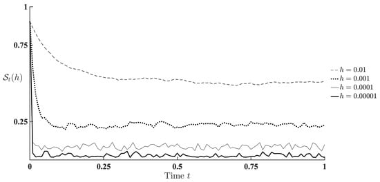
Figure 1. Estimation quality index ${\mathcal{S}}_t\left(h\right)$ depending on the time-discretization step h.

The determination of the precision order provided by the chosen numerical integration method is out of the scope of this investigation. Nevertheless, one can see the expected decrease of the estimation error when the time-discretization step descends. We appraise this result as a practical confirmation of both the theoretical assertions and numerical algorithm.

5. Conclusions

In this paper, we investigated the optimal filtering problem of the MJP states, given the indirect noisy continuous-time observations. The observation noise intensity was a function of the estimated state, so it was impossible to apply the classic Wonham filter to this observation system. To overcome this obstacle, we suggested an observation transform. On the one hand, the transformed observations remained to be equivalent to the original one from the informational point of view. On the other hand, the “new“ observations allowed to apply the effective stochastic analysis framework to process them. We derived the optimal filtering estimate theoretically as a unique strong solution to some discrete–continuous stochastic differential system. The transformed observations included derivative of the quadratic characteristics, i.e., the result of some limit passage in the stochastic settings. Hence, the subsequent numerical realization of the filtering became challenging. We proposed to approximate the initial continuous-time filtering problem by a sequence of the optimal ones given the time-discretized observations. We also involved numerical integration schemes to calculate the integrals included in the estimation formula. We prove assertions, characterizing the accuracy of the numerical approximation of the filtering estimate, i.e., the distance between the calculated approximation and optimal discrete-time filtering estimate. The accuracy depended on the observation system parameters, time discretization step, a threshold of state transition number during the time step, and the chosen scheme of the numerical integration. We suggested the whole class of numerical filtering algorithms. In each case, one could choose any specific algorithm individually, taking into account characteristics of the concrete observation system, accuracy requirements, and available computing resources.

We do not consider the presented investigations as completed. First, the characterization of the distance between the initial optimal continuous-time filtering estimate and its proposed approximation is still an open problem. Second, we can use the theoretical solution to the MJP filtering problem as a base of numerical schemes for the diffusion process filtering, given the observations with state-dependent noise. Third, the obtained optimal filtering estimate looks a springboard for a solution to the optimal stochastic control of the Markov jump processes, given both the counting and diffusion observations with state-dependent noise. All of this research is in progress.

References

- Wonham, W.M. Some Applications of Stochastic Differential Equations to Optimal Nonlinear Filtering. J. Soc. Ind. Appl. Math. Series A Control 1964, 2, 347–369. [Google Scholar] [CrossRef]
- Kalman, R.E.; Bucy, R.S. New results in linear filtering and prediction theory. Trans. ASME Ser. D J. Basic Eng. 1961, 95–108. [Google Scholar] [CrossRef]
- Rabiner, L.R. A tutorial on hidden Markov models and selected applications in speech recognition. Proc. IEEE 1989, 77, 257–286. [Google Scholar] [CrossRef]
- Ephraim, Y.; Merhav, N. Hidden Markov processes. IEEE Trans. Inf. Theory 2002, 48, 1518–1569. [Google Scholar] [CrossRef]
- Cappé, O.; Moulines, E.; Ryden, T. Inference in Hidden Markov Models; Springer: Berlin/Heidelberg, Germany, 2005. [Google Scholar]
- Elliott, R.J.; Moore, J.B.; Aggoun, L. Hidden Markov Models: Estimation and Control; Springer: New York, NY, USA, 1995. [Google Scholar]
- McLane, P.J. Optimal linear filtering for linear systems with state-dependent noise. Int. J. Control 1969, 10, 41–51. [Google Scholar] [CrossRef]
- Dragan, V.; Aberkane, S. -optimal filtering for continuous-time periodic linear stochastic systems with state-dependent noise. Syst. Control Lett. 2014, 66, 35–42. [Google Scholar] [CrossRef]
- Dragan, V.; Morozan, T.; Stoica, A. Mathematical Methods in Robust Control of Discrete-Time Linear Stochastic Systems; Springer: New York, NY, USA, 2010. [Google Scholar]
- Liptser, R.; Shiryaev, A. Statistics of Random Processes II: Applications; Springer: Berlin/Heidelberg, Germany, 2001. [Google Scholar]
- Takeuchi, Y.; Akashi, H. Least-squares state estimation of systems with state-dependent observation noise. Automatica 1985, 21, 303–313. [Google Scholar] [CrossRef]
- Joannides, M.; LeGland, F. Nonlinear filtering with continuous time perfect observations and noninformative quadratic variation. In Proceedings of the 36th IEEE Conference on Decision and Control, San Diego, CA, USA, 10–12 December 1997; Volume 2, pp. 1645–1650. [Google Scholar] [CrossRef]
- Borisov, A. Optimal filtering in systems with degenerate noise in the observations. Autom. Remote Control 1998, 59, 1526–1537. [Google Scholar]
- Crisan, D.; Kouritzin, M.; Xiong, J. Nonlinear filtering with signal dependent observation noise. Electron. J. Probab. 2009, 14, 1863–1883. [Google Scholar] [CrossRef]
- Kushner, H. Probability Methods for Approximations in Stochastic Control and for Elliptic Equations; Academic Press: New York, NY, USA, 1977. [Google Scholar]
- Kushner, H.J.; Dupuis, P.G. Numerical Methods for Stochastic Control Problems in Continuous Time; Springer: Berlin/Heidelberg, Germany, 1992. [Google Scholar]
- Ito, K.; Rozovskii, B. Approximation of the Kushner Equation for Nonlinear Filtering. SIAM J. Control Optim. 2000, 38, 893–915. [Google Scholar] [CrossRef]
- Clark, J. The design of robust approximations to the stochastic differential equations of nonlinear filtering. Commun. Syst. Random Proc. Theory 1978, 25, 721–734. [Google Scholar]
- Malcolm, W.P.; Elliott, R.J.; van der Hoek, J. On the numerical stability of time-discretised state estimation via Clark transformations. In 42nd IEEE International Conference on Decision and Control; IEEE: Piscataway, NJ, USA, 2003; Volume 2, pp. 1406–1412. [Google Scholar] [CrossRef]
- Yin, G.; Zhang, Q.; Liu, Y. Discrete-time approximation of Wonham filters. J. Control Theory Appl. 2004, 2, 1–10. [Google Scholar] [CrossRef]
- Borisov, A.V. Wonham Filtering by Observations with Multiplicative Noises. Autom. Remote Control 2018, 79, 39–50. [Google Scholar] [CrossRef]
- Borisov, A.V.; Semenikhin, K.V. State Estimation by Continuous-Time Observations in Multiplicative Noise. IFAC Pap. OnLine 2017, 50, 1601–1606. [Google Scholar] [CrossRef]
- Liptser, R.; Shiryaev, A. Theory of Martingales; Mathematics and its Applications; Springer: Dortrecht, The Netherlands, 1989. [Google Scholar]
- Stoyanov, J. Counterexamples in Probability; Wiley: Hoboken, NJ, USA, 1997. [Google Scholar]
- Kolmogorov, A.; Fomin, S. Elements of the Theory of Functions and Functional Analysis; Dover: Mineola, NY, USA, 1999. [Google Scholar]
- Platen, E.; Bruti-Liberati, N. Numerical Solution of Stochastic Differential Equations with Jumps in Finance; Springer: Berlin/Heidelberg, Germany, 2010. [Google Scholar] [CrossRef]
- Bertsekas, D.P.; Shreve, S.E. Stochastic Optimal Control: The Discrete-Time Case; Academic Press: New York, NY, USA, 1978. [Google Scholar]
- Zolotarev, V. Metric Distances in Spaces of Random Variables and Their Distributions. Math. USSR-Sbornik 1976, 30, 373–401. [Google Scholar] [CrossRef]
- Zolotarev, V. Limit Theorems as Stability Theorems. Theory Prob. Appl. 1989, 34, 153–163. [Google Scholar] [CrossRef]
- Borovkov, A. Asymptotic Methods in Queuing Theory; John Wiley & Sons: Hoboken, NJ, USA, 1984. [Google Scholar]
- Liptser, R.; Shiryaev, A. Statistics of Random Processes: I. General Theory; Springer: Berlin/Heidelberg, Germany, 2001. [Google Scholar]
© 2020 by the authors. Licensee MDPI, Basel, Switzerland. This article is an open access article distributed under the terms and conditions of the Creative Commons Attribution (CC BY) license (http://creativecommons.org/licenses/by/4.0/).