A Generic Approach to Covariance Function Estimation Using ARMA-Models

Abstract

Covariance function modeling is an essential part of stochastic methodology. Many processes in geodetic applications have rather complex, often oscillating covariance functions, where it is difficult to find corresponding analytical functions for modeling. This paper aims to give the methodological foundations for an advanced covariance modeling and elaborates a set of generic base functions which can be used for flexible covariance modeling. In particular, we provide a straightforward procedure and guidelines for a generic approach to the fitting of oscillating covariance functions to an empirical sequence of covariances. The underlying methodology is developed based on the well known properties of autoregressive processes in time series. The surprising simplicity of the proposed covariance model is that it corresponds to a finite sum of covariance functions of second-order Gauss–Markov (SOGM) processes. Furthermore, the great benefit is that the method is automated to a great extent and directly results in the appropriate model. A manual decision for a set of components is not required. Notably, the numerical method can be easily extended to ARMA-processes, which results in the same linear system of equations. Although the underlying mathematical methodology is extensively complex, the results can be obtained from a simple and straightforward numerical method.

1. Introduction and Motivation

Covariance functions are an important tool to many stochastic methods in various scientific fields. For instance, in the geodetic community, stochastic prediction or filtering is typically based on the collocation or least squares collocation theory. It is closely related to Wiener–Kolmogorov principle [1,2] as well as to the Best Linear Unbiased Predictor (BLUP) and kriging methods (e.g., [3,4,5]). Collocation is a general theory, which even allows for a change of functional within the prediction or filtering step, simply propagating the covariance to the changed functional (e.g., [6] (p. 66); [4] (pp. 171–173); [7]). In this context, signal covariance modeling is the crucial part that directly controls the quality of the stochastic prediction or filtering (e.g., [8] (Ch. 5)).

Various references on covariance functions are found in geostatistics [9,10] or atmospheric studies [11,12,13,14]. The authors in [4,5,8,15,16,17,18] cover the topic of covariance functions in the context of various geodetic applications. The discussion of types of covariance functions and investigations on positive definiteness is covered in the literature in e.g., [13,19,20,21].

In common practice, covariance modelers tend to use simple analytical models (e.g., exponential and Gauss-type) that can be easily adjusted to the first, i.e., to the short range, empirically derived covariances. Even then, as these functions are nonlinear, appropriate fitting methods are not straightforward. On the other hand, for more complex covariance models, visual diagnostics such as half-value width, correlation length, or curvature are difficult to obtain or even undefined for certain (e.g., oscillatory) covariance models. In addition, fitting procedures to any of these are sparse and lack an automated procedure (cf. [17,22]).

Autoregressive processes (AR-processes) define a causal recursive mechanism on equispaced data. Stochastic processes and autoregressive processes are covered in many textbooks in a quite unified parametrization (e.g., [23,24,25,26,27,28,29,30]). In contrast to this, various parametrizations of Autoregressive Moving Average (ARMA) processes exist in stochastic theory [31,32,33,34,35]. A general connection of these topics, i.e., stochastic processes, covariance functions, and the collocation theory in the context of geodetic usage is given by [5].

In geodesy, autoregressive processes are commonly used in the filter approach as a stochastic model within a least squares adjustment. Decorrelation procedures by digital filters derived from the parametrization of stochastic processes are widely used as they are very flexible and efficient for equidistant data (cf. e.g., [36,37,38,39,40,41,42]). Especially for highly correlated data, e.g., observations along a satellite’s orbit, advanced stochastic models can be described by stochastic processes. This is shown in the context of gravity field determination from observations of the GOCE mission with the time-wise approach, where flexible stochastic models are iteratively estimated from residuals [43,44,45].

The fact that an AR-process defines an analytical covariance sequence as well (e.g., [23]) is not well established in geostatistics and geodetic covariance modeling. To counteract this, we relate the covariance function associated with this stochastic processes to the frequently used family of covariance functions of second-order Gauss–Markov (SOGM) processes. Expressions for the covariance functions and fitting methods are aligned to mathematical equations of these stochastic process. Especially in collocation theory, a continuous covariance function is necessary to obtain covariances for arbitrary lags and functionals required for the prediction of multivariate data. However, crucially, the covariance function associated with an AR-process is in fact defined as a discrete sequence (e.g., [26]).

Whereas standard procedures which manually assess decaying exponential functions or oscillating behavior by visual inspection can miss relevant components, for instance high-frequent oscillations in the signal, the proposed method is automated and easily expandable to higher order models in order to fit components which are not obvious at first glance. A thorough modeling of a more complex covariance model does not only result in a better fit of the empirical covariances but results in a beneficial knowledge of the signal process itself.

Within this contribution, we propose an alternative method for the modeling of covariance functions based on autoregressive stochastic processes. It is shown that the derived covariance can be evaluated continuously and corresponds to a sum of well known SOGM-models. To derive the proposed modeling procedure and guidelines, the paper is organized as follows. After a general overview of the related work and the required context of stochastic modeling and collocation theory in Section 2, Section 3 summarizes the widely used SOGM-process for covariance function modeling. Basic characteristics are discussed to create the analogy to the stochastic processes, which is the key of the proposed method. Section 4 introduces the stochastic processes with a special focus on the AR-process and presents the important characteristics, especially the underlying covariance sequence in different representations. The discrete sequence of covariances is continuously interpolated by re-interpretation of the covariance sequence as a difference/differential equation, which has a continuous solution. Based on these findings, the proposed representation can be easily extended to more general ARMA-processes as it is discussed in Section 5. Whereas the previous chapters are based on the consistent definition of the covariance sequences of the processes, Section 6 shows how the derived equations and relations can be used to model covariance functions from empirically estimated covariances in a flexible and numerically simple way. In Section 7, the proposed method is applied to a one-dimensional time series which often serves as an example application for covariance modeling. The numerical example highlights the flexibility and the advantage of the generic procedure. This is followed by concluding remarks in Section 8.

2. Least Squares Collocation

In stochastic theory, a measurement model $\mathcal{L}$ is commonly seen as a stochastic process which consists of a deterministic trend $\mathit{A}\mathit{\xi }$, a random signal $\mathcal{S}$, and a white noise component $\mathcal{N}$ (cf. e.g., [3] (Ch. 2); [5] (Ch. 3.2))

$$\begin{array}{c}\hfill \mathcal{L}=\mathit{A}\mathit{\xi }+\mathcal{S}+\mathcal{N}.\end{array}$$

(1)

Whereas the signal part $\mathcal{S}$ is characterized by a covariance stationary stochastic process, the noise $\mathcal{N}$ is usually assumed as a simple white noise process with uncorrelated components. Autocovariance functions ${\gamma }^{}\left(\left|\tau \right|\right)$ or discrete sequences ${\left\{{\gamma }_{\left|j\right|}^{}\right\}}_{\Delta t}$ are models to describe the stochastic behavior of the random variables, i.e., generally ${\gamma }^{\mathcal{S}}\left(\left|\tau \right|\right)$ and ${\gamma }^{\mathcal{N}}\left(\left|\tau \right|\right)$, and are required to be positive semi-definite ([28] (Proposition 1.5.1, p. 26)). In case covariances are given as a discrete sequence ${\left\{{\gamma }_{\left|j\right|}^{}\right\}}_{\Delta t}$, they are defined at discrete lags $h=j\Delta t$ with sampling interval $\Delta t$ and $j\in {\mathbb{N}}_0$. In general, autocovariance functions or sequences are functions of a non-negative distance, here $\tau$ or h for the continuous and discrete case, respectively. Thus, covariance functions are often denoted by the absolute distance $\left|\tau \right|$ and $\left|h\right|$. Here, we introduce the conditions $\tau \ge 0$ and $h\ge 0$ in order to omit the vertical bars.

The term Least Squares Collocation, introduced in geodesy by [3,6,46], represents the separability problem within the remove–restore technique, where a deterministic estimated trend component $\mathit{A}\tilde{\mathit{x}}$ is subtracted from the measurements ℓ and the remainder $\widetilde{\Delta \mathit{\ell }}=\mathit{\ell }-\mathit{A}\tilde{\mathit{x}}$ is interpreted as a special realization of the stochastic process $\widetilde{\Delta \mathcal{L}}$. In the trend estimation step

$$\tilde{\mathit{x}}={\left({\mathit{A}}^T{({\mathsf{\Sigma }}_{\mathcal{S}\mathcal{S}}+{\mathsf{\Sigma }}_{\mathcal{N}\mathcal{N}})}^{-1}\mathit{A}\right)}^{-1}{\mathit{A}}^T{({\mathsf{\Sigma }}_{\mathcal{S}\mathcal{S}}+{\mathsf{\Sigma }}_{\mathcal{N}\mathcal{N}})}^{-1}\mathit{\ell },$$

(2)

the optimal parameter vector $\tilde{\mathit{x}}$ is computed from the measurements ℓ as the best linear unbiased estimator (BLUE) for the true trend $\mathit{A}\mathit{\xi }$. The collocation step follows as the best linear unbiased predictor (BLUP) of the stochastic signal $\tilde{\mathit{s}}{}^{\prime }$ at arbitrary points

$$\tilde{\mathit{s}}{}^{\prime }={\mathsf{\Sigma }}_{{\mathcal{S}}^{\prime }\mathcal{S}}{({\mathsf{\Sigma }}_{\mathcal{S}\mathcal{S}}+{\mathsf{\Sigma }}_{\mathcal{N}\mathcal{N}})}^{-1}\widetilde{\Delta \mathit{\ell }}$$

(3)

or as a filter process at the measured points

$$\tilde{\mathit{s}}={\mathsf{\Sigma }}_{\mathcal{S}\mathcal{S}}{({\mathsf{\Sigma }}_{\mathcal{S}\mathcal{S}}+{\mathsf{\Sigma }}_{\mathcal{N}\mathcal{N}})}^{-1}\widetilde{\Delta \mathit{\ell }}$$

(4)

([3] (Ch. 2); [5] (Ch. 3)). The variance/covariance matrices ${\mathsf{\Sigma }}_{\mathcal{S}\mathcal{S}}$ reflect the stochastic behavior of the random signal $\mathcal{S}$. The coefficients are derived by the evaluation of the covariance function ${\gamma }^{\mathcal{S}}\left(\tau \right)$, where $\tau$ represents the lags or distances between the corresponding measurement points. ${\mathsf{\Sigma }}_{\mathcal{N}\mathcal{N}}$ denotes the variances/covariances of the random noise which is often modeled as independent and identically distributed random process, ${\gamma }^{\mathcal{N}}\left(\tau \right)={\delta }_{0,\tau }{\sigma }_{\mathcal{N}}^2$ with ${\delta }_{i,j}$ being the Kronecker delta. ${\sigma }_{\mathcal{N}}^2$ denotes the variance of the noise such that the covariance matrix reads ${\mathsf{\Sigma }}_{\mathcal{N}\mathcal{N}}=\mathsf{𝟙}{\sigma }_{\mathcal{N}}^2$. ${\mathsf{\Sigma }}_{{\mathcal{S}}^{\prime }\mathcal{S}}$ is filled row-wise with the covariances of the signal between the prediction points and the measured points.

The true covariance functions ${\gamma }^{\mathcal{S}}\left(\tau \right)$ and ${\gamma }^{\mathcal{N}}\left(\tau \right)$ are unknown and often have to be estimated, i.e., $g^{\mathcal{S}}\left(\tau \right)$ and $g^{\mathcal{N}}\left(\tau \right)$, directly from the trend reduced measurements $\Delta \mathit{\ell }$ by an estimation procedure using the empirical covariance sequences ${\left\{{\tilde{g}}_j^{\Delta \mathcal{L}}\right\}}_{\Delta t}$. The estimated noise variance ${\tilde{s}}_{\mathcal{N}}^2$ can be derived from the empirical covariances at lag zero

$${\tilde{g}}_0^{\Delta \mathcal{L}}={\tilde{g}}_0^{\mathcal{S}}+{\tilde{s}}_{\mathcal{N}}^2.$$

(5)

Thus, it is allowed to split up ${\tilde{g}}_0^{\Delta \mathcal{L}}$ into the signal variance ${\tilde{g}}_0^{\mathcal{S}}$ given by the covariance function $g^{\mathcal{S}}\left(0\right)={\tilde{g}}_0^{\mathcal{S}}$ and a white noise component ${\tilde{s}}_{\mathcal{N}}^2$, known as the nugget effect (e.g., [9] (p. 59)). In theory, ${\tilde{s}}_{\mathcal{N}}^2$ can be manually chosen such that the function plausibly decreases from ${\tilde{g}}_0^{\mathcal{S}}$ towards ${\tilde{g}}_1^{\mathcal{S}}$ and the higher lags. A more elegant way is to estimate the analytical function $g^{\mathcal{S}}\left(\tau \right)$ from empirical covariances ${\tilde{g}}_j^{\mathcal{S}}$ with $j>0$ only. Naturally, all estimated functions $g^{\mathcal{S}}\left(\tau \right)$ must result in ${\tilde{g}}_0^{\Delta \mathcal{L}}-g^{\mathcal{S}}\left(0\right)\ge 0$.

Covariance function modeling is a task in various fields of application. They are used for example to represent a stochastic model of the observations within parameter estimation in e.g., laserscanning [18], GPS [47,48], or gravity field modeling [49,50,51,52,53,54]. The collocation approach is closely related to Gaussian Process Regression from the machine learning domain [55]. The family of covariance functions presented here can be naturally used as kernel functions in such approaches.

Within these kinds of applications, the covariance functions are typically fitted to empirically derived covariances which follow from post-fit residuals. Within an iterative procedure, the stochastic model can be refined. Furthermore, they are used to characterize the signal characteristics, again e.g., in gravity field estimation or geoid determination in the context of least squares collocation [7] or in atmospheric sciences [11,14].

Reference [8] (Ch. 3) proposed to have a special look to only the three parameters, variance, correlation length, and curvature at the origin to fit a covariance function to the empirical covariance sequence. Reference [17] also suggested taking the sequence of zero crossings into account to find an appropriate set of base functions. In addition, most approaches proceed with the fixing of appropriate base functions for the covariance model as a first step. This step corresponds to the determination of the type or family of the covariance function. The fitting then is restricted to this model and does not generalize well to other and more complex cases. Furthermore, it is common to manually fix certain parameters and optimize only a subset parameters in an adjustment procedure; see e.g., [18].

Once the covariance model is fixed, various optimization procedures exist to derive the model parameters which result in a best fit of the model to a set of empirical covariances. Thus, another aspect of covariance function estimation is the numerical implementation of the estimation procedure. Visual strategies versus least squares versus Maximum Likelihood, point cloud versus representative empirical covariance sequences and non robust versus robust estimators are various implementation possibilities discussed in the literature (see e.g., [11,14,18,47,51,56]). To summarize, the general challenges of covariance function fitting are to find an appropriate set of linear independent base functions, i.e., the type of covariance function, and the nonlinear nature of the set of chosen base functions together with the common problem of outlier detection and finding good initial values for the estimation process.

In particular, geodetic data often exhibit negative correlations or even oscillatory behavior in the covariance functions which leaves a rather limited field of types of covariance functions, e.g., cosine and cardinal sine functions in the one-dimensional or Bessel functions in two-dimensional case (e.g., [27]). One general class of covariance functions with oscillatory behavior is discussed in the next section.

3. The Second-Order Gauss–Markov Process

3.1. The Covariance Function of the SOGM-Process

A widely used covariance function is based on the second-order Gauss–Markov processes as given in [23] (Equation (5.2.36)) and [25] (Ch. 4.11, p. 185). The process defines a covariance function of the form

$$\begin{array}{c}\hfill \begin{array}{cc}\hfill \gamma \left(\tau \right)& =\frac{{\sigma }^2}{cos\left(\eta \right)}{\mathrm{e}}^{-\zeta {\omega }_0\tau }cos\left(\sqrt{1-{\zeta }^2}{\omega }_0\tau -\eta \right)\hfill \\ \hfill & =\begin{array}{c}\hfill \left[t\right]{\sigma }^2{\mathrm{e}}^{-\zeta {\omega }_0\tau }\left(cos\left(\sqrt{1-{\zeta }^2}{\omega }_0\tau \right)+tan\left(\eta \right)sin\left(\sqrt{1-{\zeta }^2}{\omega }_0\tau \right)\right)\end{array}\hfill \\ \hfill & \hfill \mathrm{with}0<\zeta <1\mathrm{and}{\omega }_0>0.\end{array}\end{array}$$

(6)

Its shape is defined by three parameters. ${\omega }_0$ represents a frequency and $\zeta$ is related to the attenuation. The phase $\eta$ can be restricted to the domain $\left|\eta \right|<\pi /2$ for logical reasons.

A reparametrization with $c:=\zeta {\omega }_0$ and $a:=\sqrt{1-{\zeta }^2}{\omega }_0$ gives

$$\begin{array}{c}\hfill \begin{array}{cc}\hfill \gamma \left(\tau \right)& =\frac{{\sigma }^2}{cos\left(\eta \right)}{\mathrm{e}}^{-c\tau }cos\left(a\tau -\eta \right)\hfill \\ \hfill & ={\sigma }^2{\mathrm{e}}^{-c\tau }\left(cos\left(a\tau \right)+tan\left(\eta \right)sin\left(a\tau \right)\right)\mathrm{with}a,c>0\hfill \end{array}\end{array}$$

(7)

which highlights the shape of a sinusoid. We distinguish between the nominal frequency a and the natural frequency ${\omega }_0=a/\sqrt{1-{\zeta }^2}$. The relative weight of the sine with respect to the cosine term amounts to $w:=tan\left(\eta \right)$. It is noted here that the SOGM-process is uniquely defined by three parameters. Here, we will use ${\omega }_0$, $\zeta$ and $\eta$ as the defining parameters. Of course, the variance ${\sigma }^2$ is a parameter as well. However, as it is just a scale and remains independent of the other three, it is not relevant for the theoretical characteristics of the covariance function.

The described covariance function is referenced by various names, e.g., the second-order shaping filter [57], the general damped oscillation curve [27] (Equation (2.116)), and the underdamped second-order continuous-time bandpass filter [58] (p. 270). In fact, the SOGM represents the most general damped oscillating autocorrelation function built from exponential and trigonometric terms. For example, the function finds application in VLBI analysis [59,60].

3.2. Positive Definiteness of the SOGM-Process

At first glance, it is surprising that a damped sine term is allowed in the definition of the covariance function of the SOGM-process (cf. Equation (6)), as the sine is not positive semi-definite. However, it is shown here that it is in fact a valid covariance function, provided that some conditions on the parameters are fulfilled.

The evaluation concerning the positive semi-definiteness of the second-order Gauss–Markov process can be derived by analyzing the process’s Fourier transform as given in [25] (Ch. 4.11, p. 185) and the evaluation of it being non-negative (cf. the Bochner theorem, [61]). The topic is discussed and summarized in [60]. With some natural requirements already enforced by $0\le \zeta \le 1$ and ${\omega }_0>0$, the condition for positive semi-definiteness (cf. e.g., [57] (Equation (A2))) is

$$\begin{array}{c}\hfill |sin(\eta \left)\right|\le \zeta \end{array}$$

(8)

which can be expressed by the auxiliary variable $\alpha :=arcsin\left(\zeta \right)$ as $\left|\eta \right|\le \alpha$.

In terms of the alternative parameters a and c, this condition translates to $w\le c/a$ (cf. e.g., [27] (Equation (2.117))). As a result, non-positive definite functions as the sine term are allowed in the covariance function only if the relative contribution compared to the corresponding cosine term is small enough.

4. Discrete AR-Processes

4.1. Definition of the Process

A more general and more flexible stochastic process is defined by the autoregressive (AR) process. An AR-process is a time series model which relates signal time series values, or more specifically the signal sequence, ${\mathcal{S}}_i$ with autoregressive coefficients ${\alpha }_k$ as (e.g., [26] (Ch. 3.5.4))

$$\begin{array}{c}\hfill {\mathcal{S}}_i=\sum _{k=1}^p{\alpha }_k{\mathcal{S}}_{i-k}+{\mathcal{E}}_i.\end{array}$$

(9)

With the transition to ${\overline{\alpha }}_0:=1$, ${\overline{\alpha }}_1:=-{\alpha }_1$, ${\overline{\alpha }}_2:=-{\alpha }_2$, etc., the decorrelation relation to white noise ${\mathcal{E}}_i$ is given by

$$\begin{array}{c}\hfill \sum _{k=0}^p{\overline{\alpha }}_k{\mathcal{S}}_{i-k}={\mathcal{E}}_i.\end{array}$$

(10)

The characteristic polynomial in the factorized form (cf. [26] (Ch. 3.5.4))

$$\begin{array}{c}\hfill {\overline{\alpha }}_0{x}^p+{\overline{\alpha }}_1{x}^{p-1}+\cdots +{\overline{\alpha }}_p=\prod _{k=1}^p(x-p_k)\end{array}$$

(11)

has the roots $p_k\in \mathbb{C}$, i.e., the poles of the autoregressive process, which can be complex numbers. This defines a unique transition between coefficients and poles. In common practice, the poles of an AR(p)-process only appear as a single real pole or as complex conjugate pairs. Following this, an exemplary process of order $p=4$ can be composed by either two complex conjugate pairs, or one complex pair and two real poles, or four individual single real poles. An odd order gives at least on real pole. For general use, AR-processes are required to be stationary. This requires that its poles are inside the unit circle, i.e., $\left|p_k\right|<1$ (cf. [26] (Ch. 3.5.4)).

AR-processes define an underlying covariance function as well. We will provide it analytically for the AR(2)-process and will summarize a computation strategy for the higher order processes in the following.

4.2. The Covariance Function of the AR(2)-Process

Although AR-processes are defined by discrete covariance sequences, the covariance function can be written as a closed analytic expression, which, evaluated at the discrete lags, gives exactly the discrete covariances. For instance, the AR(2)-process has a covariance function which can be written in analytical form. The variance of AR-processes is mostly parameterized using the variance ${\sigma }_{\mathcal{E}}^2$ of the innovation sequence ${\mathcal{E}}_i$. In this paper, however, we use a representation with the autocorrelation function and a variance ${\sigma }^2$ as in [26] (Equation (3.5.36), p. 130) and [62] (Section 3.5, p. 504). In addition, the autoregressive parameters ${\alpha }_1$ and ${\alpha }_2$ can be converted to the parameters a and c via $a=arccos\left({\alpha }_1/\left(2\sqrt{-{\alpha }_2}\right)\right)$ and $c=-\ln \left(\sqrt{-{\alpha }_2}\right)$. Hence, the covariance function of the AR(2)-process can be written in a somewhat complicated expression in the variables a and c as

$$\begin{array}{c}\hfill \gamma \left(\tau \right)={\sigma }^2\sqrt{{\left(cot\left(a\right)tanh\left(c\right)\right)}^2+1}{\mathrm{e}}^{-c\tau }cos\left(a\tau -arctan\left(cot\left(a\right)tanh\left(c\right)\right)\right)\end{array}$$

(12)

using the phase $\eta =arctan(cot(a)tanh(c\left)\right)$ or likewise

$$\begin{array}{c}\hfill \gamma \left(\tau \right)={\sigma }^2{\mathrm{e}}^{-c\tau }\left(cos\left(a\tau \right)+tanh\left(c\right)cot\left(a\right)sin\left(a\tau \right)\right)\end{array}$$

(13)

with the weight of the sine term $w=tanh\left(c\right)cot\left(a\right)$.

Please note that in contrast to the SOGM-process the weight or phase in Equations (12) and (13) cannot be set independently, but depends on a and c. Thus, this model is defined by two parameters only. Therefore, the SOGM-process is the more general model. Caution must be used with respect to the so-called second-order autoregressive covariance model of [11], which is closely related but does not correspond to the standard discrete AR-process.

4.3. AR(p)-Process

The covariance function of an AR(p)-process is given as a discrete series of covariances ${\left\{{\gamma }_j\right\}}_{\Delta t}$ defined at discrete lags $h=j\Delta t$ with distance $\Delta t$. The Yule–Walker equations (e.g., [24] (Section 3.2); [30] (Equation (11.8)))

(14)

directly relate the covariance sequence to the AR(p) coefficients. With (14a) being the 0th equation, the next p Yule–Walker equations (first to pth, i.e., (14b)) are the linear system mostly used for estimation of the autoregressive coefficients. Note that this system qualifies for the use of Levinson–Durbin algorithm because it is Toeplitz structured, cf. [30] (Ch. 11.3) and [63].

The linear system containing only the higher equations (14c) is called the modified Yule–Walker (MYW) equations, cf. [64]. This defines an overdetermined system which can be used for estimating the AR-process parameters where n lags are included.

The recursive relation

$$\begin{array}{c}\hfill {\gamma }_i-{\alpha }_1{\gamma }_{i-1}-{\alpha }_2{\gamma }_{i-2}-\dots -{\alpha }_p{\gamma }_{i-p}=0,\mathrm{for}i=p+1,p+2,\dots \end{array}$$

(15)

represents a pth order linear homogeneous difference equation whose general solution is given by the following equation with respect to a discrete and equidistant time lag $h=|t-t^{\prime }|=j\Delta t$

$$\begin{array}{c}\hfill {\gamma }_j=A_1{p}_1^h+A_2{p}_2^h+\dots +A_p{p}_p^h\mathrm{with}j\in {\mathbb{N}}_0,h\in {\mathbb{R}}^{+},A_k\in \mathbb{C},\end{array}$$

(16)

cf. [23] (Equation (5.2.44)) and [26] (Equation (3.5.44)). $p_k$ are the poles of the process (cf. Equation (11)) and $A_k$ some unknown coefficients.

It has to be noted here that covariances of AR(p)-processes are generally only defined at discrete lags. However, it can be mathematically shown that the analytic function of Equation (13) exactly corresponds to the covariance function Equation (6) of the SOGM. In other words, the interpolation of the discrete covariances is done using the same sinusoidal functions as in Equation (6) such that the covariance function of the AR(p)-process can equally be written with respect to a continuous time lag $\tau =|t-t^{\prime }|$ by

$$\begin{array}{c}\hfill \gamma \left(\tau \right)=\mathrm{Re}\left(A_1{p}_1^{\tau }+A_2{p}_2^{\tau }+\dots +A_p{p}_p^{\tau }\right)=\mathrm{Re}\left(\sum _{k=1}^p{A}_k{p}_k^{\tau }\right)\mathrm{with}\tau \in {\mathbb{R}}^{+},A_k\in \mathbb{C}.\end{array}$$

(17)

This is also a valid solution of Equation (15) in the sense that $\gamma \left(h\right)={\gamma }_j$ holds. For one special case of poles, which are negative real poles, the function can be complex valued due to the continuous argument $\tau$. Thus, the real part has to be taken for general use.

Now, assuming $A_k$ and $p_k$ to be known, Equation (17) can be used to interpolate the covariance defined by an AR-process for any lag $\tau$. Consequently, the covariance definition of an AR-process leads to an analytic covariance function which can be used to interpolate or approximate discrete covariances.

4.3.1. AR(2)-Model

We can investigate the computation for the processes of second order in detail. Exponentiating a complex number mathematically corresponds to

$$\begin{array}{c}\hfill p_k^{\tau }={\left|p_k\right|}^{\tau }\left(cos\left(\arg \left(p_k\right)\tau \right)+isin\left(\arg \left(p_k\right)\tau \right)\right).\end{array}$$

(18)

As complex poles always appear in conjugate pairs, it is plausible that for complex conjugate pairs $p_k=p_l^{{}^{*}}$ the coefficients $A_k$ and $A_l$ are complex and also conjugate to each other $A_k=A_l^{{}^{*}}$. Thus, $A_k{p}_k^{\tau }+A_l{p}_l^{\tau }$ becomes $A_k{p}_k^{\tau }+A_k^{{}^{*}}{\left(p_k^{{}^{*}}\right)}^{\tau }$ and the result will be real.

From Equation (13), we can derive that the constants amount to $A_{k,l}=\frac{{\sigma }^2}{2}\left(1\pm itanh\left(c\right)cot\left(a\right)\right)=\frac{{\sigma }^2}{2}\left(1\pm iw\right)$ for the AR(2)-process and from Equation (18) we can see that $c=-\ln \left(\left|p_k\right|\right)$ and $a=\left|\arg \left(p_k\right)\right|$ such that the covariance function can be written as

$$\begin{array}{l}\gamma (\tau )={\sigma }^2\sqrt{{\left(tanh\left(\ln \left(\left|p_k\right|\right)\right)cot\left(\left|\arg \left(p_k\right)\right|\right)\right)}^2+1}\\ {\left|p_k\right|}^{\tau }cos\left(\left|\arg \left(p_k\right)\right|\tau +arctan\left(tanh\left(\ln \left(\left|p_k\right|\right)\right)cot\left(\left|\arg \left(p_k\right)\right|\right)\right)\right)\end{array}$$

(19)

$$\begin{array}{cc}\hfill & ={\sigma }^2{\left|p_k\right|}^{\tau }\left(cos\left(\left|\arg \left(p_k\right)\right|\tau \right)-tanh\left(\ln \left(\left|p_k\right|\right)\right)cot\left(\left|\arg \left(p_k\right)\right|\right)sin\left(\left|\arg \left(p_k\right)\right|\tau \right)\right).\hfill \end{array}$$

(20)

It is evident now that the AR(2) covariance model can be expressed as an SOGM covariance function. Whilst the SOGM-process has three independent parameters, here, both damping, frequency, and phase of Equation (19) are determined by only two parameters $\left|p_k\right|$ and $\left|\arg \left(p_k\right)\right|$ based on ${\mathrm{e}}^{-c}=\left|p_k\right|$, $c=-\ln \left(\left|p_k\right|\right)$, $a=\left|\arg \left(p_k\right)\right|$ and $\eta =arctan\left(tanh\left(\ln \left(\left|p_k\right|\right)\right)cot\left(\left|\arg \left(p_k\right)\right|\right)\right)$. Thus, the SOGM-process is the more general model, whereas the AR(2)-process has a phase $\eta$ or weight w that is not independent. From Equation (19), phase $\eta$ can be recovered from the $A_k$ by

$$\begin{array}{c}\hfill \left|{\eta }_k\right|=\left|\arg \left(A_k\right)\right|\end{array}$$

(21)

and the weight by $\left|w\right|=\left|\mathrm{Im}\left(A_k\right)/\mathrm{Re}\left(A_k\right)\right|$.

4.3.2. AR(1)-Model

Here, the AR(1)-model appears as a limit case. Exponentiating a positive real pole results in exponentially decaying behavior. Thus, for a single real positive pole, one directly gets the exponential Markov-type AR(1) covariance function, also known in the literature as first-order Gauss–Markov (FOGM), cf. [65] (p. 81). A negative real pole causes discrete covariances of alternating sign. In summary, the AR(1)-process gives the exponentially decaying covariance function for $0<p_k<1$

$$\begin{array}{c}\hfill \begin{array}{cc}\hfill \gamma \left(\tau \right)& ={\sigma }^{2}exp\left(-c\tau \right)\mathrm{with}c=-\ln \left(\left|p_k\right|\right)\hfill \\ \hfill & ={\sigma }^2{\left|p_k\right|}^{\tau }\hfill \end{array}\end{array}$$

(22)

or the exponentially decaying oscillation with Nyquist frequency for $-1<p_k<0$, cf. [23] (p. 163), i.e.,

$$\begin{array}{c}\hfill \begin{array}{cc}\hfill \gamma \left(\tau \right)& ={\sigma }^{2}exp\left(-c\tau \right)cos\left(\pi \tau \right)\hfill \\ \hfill & ={\sigma }^2{\left|p_k\right|}^{\tau }cos\left(\pi \tau \right).\hfill \end{array}\end{array}$$

(23)

4.4. Summary

From Equation (17), one can set up a linear system

$$\begin{array}{c}\hfill \left[\begin{array}{c}{\gamma }_0\hfill \\ {\gamma }_1\hfill \\ {\gamma }_2\hfill \\ {\gamma }_3\hfill \end{array}\right]=\left[\begin{array}{cccc}{p}_1^0\hfill & p_2^0\hfill & p_3^0\hfill & p_4^0\hfill \\ p_1^1\hfill & p_2^1\hfill & p_3^1\hfill & p_4^1\hfill \\ p_1^2\hfill & p_2^2\hfill & p_3^2\hfill & p_4^2\hfill \\ p_1^3\hfill & p_2^3\hfill & p_3^3\hfill & p_4^3\hfill \end{array}\right]\left[\begin{array}{c}{A}_1\hfill \\ A_2\hfill \\ A_3\hfill \\ A_4\hfill \end{array}\right]\mathrm{or}\left[\begin{array}{c}{\gamma }_1\hfill \\ {\gamma }_2\hfill \\ {\gamma }_3\hfill \\ {\gamma }_4\hfill \end{array}\right]=\left[\begin{array}{cccc}{p}_1^1\hfill & p_2^1\hfill & p_3^1\hfill & p_4^1\hfill \\ p_1^2\hfill & p_2^2\hfill & p_3^2\hfill & p_4^2\hfill \\ p_1^3\hfill & p_2^3\hfill & p_3^3\hfill & p_4^3\hfill \\ p_1^4\hfill & p_2^4\hfill & p_3^4\hfill & p_4^4\hfill \end{array}\right]\left[\begin{array}{c}{A}_1\hfill \\ A_2\hfill \\ A_3\hfill \\ A_4\hfill \end{array}\right],\end{array}$$

(24)

here shown exemplarily for an AR(4)-process. The solution of Equation (24) uniquely determines the constants $A_k$ applying standard numerical solvers, assuming the poles to be known from the process coefficients, see Equation (11).

Since Equation (17) is a finite sum over exponentiated poles, the covariance function of a general AR(p)-process is a sum of, in case of complex conjugate pairs, AR(2)-processes in the shape of Equation (19) or, in case of real poles, damping terms as given in Equations (22) and (23). The great advantage is that the choice of poles is automatically done by the estimation of the autoregressive process by the YW-Equations (14). Here, we also see that the AR(2)-process as well as both cases of the AR(1)-process can be modeled with Equation (17) such that the proposed approach automatically handles both cases.

Furthermore, we see that Equation (17) adds up the covariance functions of the forms of Equation (19), Equation (22), or Equation (23) for each pole or pair of poles. Any recursive filter can be uniquely dissected into a cascade of second-order recursive filters, described as second-order sections (SOS) or biquadratic filter, cf. [58] (Ch. 11). Correspondingly, the poles of amount p can be grouped into complex-conjugate pairs or single real poles. Thus, the higher order model is achieved by concatenation of the single or paired poles into the set of p poles (vector p) and correspondingly by adding up one SOGM covariance function for each section. Nonetheless, this is automatically done by Equation (17).

5. Generalization to ARMA-Models

5.1. Covariance Representation of ARMA-Processes

Thus far, we introduced fitting procedures for the estimation of autoregressive coefficients as well as a linear system of equations to simply parameterize the covariance function of AR(p)-processes. In this section, we demonstrate that ARMA-models can be handled with the same linear system and the fitting procedure thus generalizes to ARMA-processes.

For the upcoming part, it is crucial to understand that the exponentiation $p_k^{\tau }$ of Equation (17) exactly corresponds to the exponentiation defined in the following way:

$$\begin{array}{cc}\hfill {\mathrm{e}}^{s_k\tau }& ={\mathrm{e}}^{\mathrm{Re}\left(s_k\right)\tau }\left(cos\left(\mathrm{Im}\left(s_k\right)\tau \right)+isin\left(\mathrm{Im}\left(s_k\right)\tau \right)\right)\hfill \end{array}$$

(25)

i.e., $p_k^{\tau }={\mathrm{e}}^{s_k\tau }$, if the transition between the poles $p_k$ to $s_k$ is done by $s_k=ln\left(p_k\right)=\left(ln\left(\left|p_k\right|\right)+i\arg \left(p_k\right)\right)$ and $p_k={\mathrm{e}}^{s_k}$. To be exact, this denotes the transition of the poles from the z-domain to the Laplace-domain. This parametrization of the autoregressive poles can, for example, be found in [23] (Equation (5.2.46)), [66] (Equation (A.2)), and [26] (Equation (3.7.58)). In these references, the covariance function of the AR-process is given as a continuous function with respect to the poles $s_k$ such that the use of Equation (17) as a continuous function is also justified.

In the literature, several parametrizations of the moving average part exist. Here, we analyze the implementation of [33] (Equation (2.15)), where the covariance function of an ARMA-process is given by

$$\begin{array}{cc}\hfill \gamma \left(\tau \right)& =\sum _{k=1}^p\frac{b\left(s_k\right)b\left(-s_k\right)}{a^{\prime }\left(s_k\right)a\left(-s_k\right)}{\mathrm{e}}^{s_k\tau }.\hfill \end{array}$$

(26)

Inserting $p_k^{\tau }={\mathrm{e}}^{s_k\tau }$ and denoting $A_k:=\frac{b\left(s_k\right)b(-s_k)}{a^{\prime }\left(s_k\right)a(-s_k)}$ which is independent of $\tau$, we obtain

$$\begin{array}{c}\hfill \gamma \left(\tau \right)=\sum _{k=1}^p\frac{b\left(s_k\right)b\left(-s_k\right)}{a^{\prime }\left(s_k\right)a\left(-s_k\right)}{p}_k^{\tau }=\sum _{k=1}^p{A}_k{p}_k^{\tau },\end{array}$$

(27)

which is suitable for the purpose of understanding the parametrization chosen in this paper. Now, the covariance corresponds to the representation of Equation (17). The equation is constructed by a finite sum of complex exponential functions weighted by a term consisting of some polynomials $a\left(·\right)$, $a^{\prime }\left(·\right)$ for the AR-part and $b\left(·\right)$ for the MA-part evaluated at the positions of the positive and negative autoregressive roots $s_k$.

It is evident in Equation (26) that $\tau$ is only linked with the poles. This exponentiation of the poles builds the term which is responsible for the damped oscillating or solely damping behavior. The fraction builds the weighting of these oscillations exactly the same way as the $A_k$ in Equation (17). In fact, Equation (17) can undergo a partial fraction decomposition and be represented as in Equation (26). The main conclusion is that ARMA-models can also be realized with Equation (17). The same implication is also gained from the parametrizations by [67] (Equation (3.2)), [31] (Equation (48)), [68] (Equation (9)), and [34] (Equation (4)). It is noted here that the moving average parametrization varies to a great extent in the literature in the sense that very different characteristic equations and zero and pole representations are chosen.

As a result, although the MA-part is extensively more complex than the AR-part and very differently modeled throughout the literature, the MA-parameters solely influence the coefficients $A_k$ weighting the exponential terms, which themselves are solely determined by the autoregressive part. This is congruent with the findings of the Equation (19) where frequency and damping of the SOGM-process are encoded into the autoregressive poles $p_k$.

5.2. The Numerical Solution for ARMA-Models

Autoregressive processes of order p have the property that $p+1$ covariances are uniquely given by the process, i.e., by the coefficients and the variance. All higher model-covariances can be recursively computed from the previous ones, cf. Equation (15). This property generally does not hold for empirical covariances, where each covariance typically is an independent estimate. Now, suppose Equation (24) is solved as an overdetermined system by including higher empirical covariances, i.e., covariances that are not recursively defined. The resulting weights $A_k$ will automatically correspond to general ARMA-models because the poles $p_k$ are fixed.

Precisely, the contradiction within the overdetermined system will, to some extent, forcedly end up in the weights $A_k$ and thus in some, for the moment unknown, MA-coefficients. The model still is an SOGM process because the number of poles is still two and the SOGM covariance function is the most general damped oscillating function. The two AR-poles uniquely define the two SOGM-parameters frequency ${\omega }_0$ and attenuation $\zeta$. The only free parameter to fit an ARMA-model into the shape of the general damped oscillating function (SOGM-process) is the phase $\eta$. Hence, the MA-part of arbitrary order will only result in a single weight or phase as in Equation (19) and the whole covariance function can be represented by an SOGM-process. Consequently, the $A_k$ will be different from that of Equation (20), cf. [29] (p. 60), but the phase can still be recovered from Equation (21).

In summary, the general ARMA(2,q)-model (Equation (26)) is also realizable with Equation (17) and thus with the linear system of Equation (24). Here, we repeat the concept of second-order sections. Any ARMA(p,q)-process can be uniquely dissected into ARMA(2,2)-processes. Thus, our parametrization of linear weights to complex exponentials can realize pure AR(2) and general SOGM-processes, which can be denoted as ARMA(2,q)-models. These ARMA(2,q)-processes form single SOGM-processes with corresponding parameters ${\omega }_0$, $\zeta$ and $\eta$. The combination of the ARMA(2,q) to the original ARMA(p,q) process is the operation of addition for the covariance (function), concatenation for the poles, and convolution for the coefficients. Thus, the expansion to higher orders is similar to the pure AR(p) case. The finite sum adds up the covariance function for each second-order section which is an SOGM-process.

The weights would have to undergo a partial-fraction decomposition to give the MA-coefficients. Several references exist for decomposing Equation (26) into the MA-coefficients, known as spectral factorization, e.g., by partial fraction decomposition. In this paper, we stay with the simplicity and elegance of Equation (17).

6. Estimation and Interpolation of the Covariance Series

Within this section, the theory summarized above is used for covariance modeling, i.e., estimating covariance functions $g^{\mathcal{S}}\left(\tau \right)$, which can be evaluated for any lag $\tau$, from a sequence of given empirical covariances ${\left\{{\tilde{g}}_j^{\Delta \mathcal{L}}\right\}}_{\Delta t}$. Here, the choice of estimator for the empirical covariances is not discussed and it is left to the user whether to use the biased or the unbiased estimator of the empirical covariances, cf. [23] (p. 174) and [69] (p. 252).

The first step is the estimation of the process coefficients from the ${\tilde{g}}_j^{\Delta \mathcal{L}}$ with the process order p defined by the user. Furthermore, different linear systems have been discussed for this step, cf. Equation (14), also depending on the choice of n, which is the index of the highest lag included in Equation (14). These choices already have a significant impact on the goodness of fit of the covariance function to the empirical covariances, as will be discussed later. The resulting AR-coefficients ${\alpha }_k$ can be directly converted to the poles $p_k$ using the factorization of the characteristic polynomial (Equation (11)).

For the second step, based on Equation (16), a linear system of m equations with $m\ge p$, can be set up, but now for the empirical covariances. Using the first m covariances, but ignoring the lag 0 value contaminated by the nugget effect, this results in a system like Equation (24), but now in the empirical covariances ${\tilde{g}}_j^{\Delta \mathcal{L}}={\tilde{g}}_j^{\mathcal{S}},j>0$

$$\begin{array}{c}\hfill \left[\begin{array}{c}{\tilde{g}}_1^{\mathcal{S}}\hfill \\ {\tilde{g}}_2^{\mathcal{S}}\hfill \\ ⋮\hfill \\ {\tilde{g}}_{m-1}^{\mathcal{S}}\hfill \\ {\tilde{g}}_m^{\mathcal{S}}\hfill \end{array}\right]=\left[\begin{array}{ccccc}{p}_1^1\hfill & p_2^1\hfill & \cdots \hfill & p_{p-1}^1\hfill & p_p^1\hfill \\ p_1^2\hfill & p_2^2\hfill & \cdots \hfill & p_{p-1}^2\hfill & p_p^2\hfill \\ ⋮\hfill & ⋮\hfill & \hfill & ⋮\hfill & ⋮\hfill \\ p_1^{m-1}\hfill & p_2^{m-1}\hfill & \cdots \hfill & p_{p-1}^{m-1}\hfill & p_p^{m-1}\hfill \\ p_1^m\hfill & p_2^m\hfill & \cdots \hfill & p_{p-1}^m\hfill & p_p^m\hfill \end{array}\right]\left[\begin{array}{c}{A}_1\hfill \\ A_2\hfill \\ ⋮\hfill \\ A_{p-1}\hfill \\ A_p\hfill \end{array}\right].\end{array}$$

(28)

For $m=p$, the system can be uniquely solved, resulting in coefficients $A_k$ which model the covariance function as an AR(p)-process. The case $m>p$ results in a fitting problem of the covariance model to the m empirical covariances ${\tilde{g}}_j$ with p unknowns. This overdetermined system can be solved for instance in the least squares sense to derive estimates $A_k$ from the ${\tilde{g}}_j$. As was discussed, these $A_k$ signify a process modeling as an ARMA-model. Here, one could use the notation ${\tilde{A}}_k$ in order to indicate adjusted parameters in contrast to the uniquely determined $A_k$ for the pure AR-process. For the sake of a unified notation of Equation (17), it is omitted.

Due to the possible nugget effect, it is advised to exclude ${\tilde{g}}_0^{\Delta \mathcal{L}}$ and solve Equation (28); however, it can also be included, cf. Equation (24). Moreover, a possible procedure can be to generate a plausible ${\tilde{g}}_0^{\mathcal{S}}$ from a manually determined ${\tilde{s}}_{\mathcal{N}}^2$ by ${\tilde{g}}_0^{\mathcal{S}}={\tilde{g}}_0^{\Delta \mathcal{L}}-{\tilde{s}}_{\mathcal{N}}^2$. Equally, the MYW-Equations are a possibility to circumvent using ${\tilde{g}}_0^{\Delta \mathcal{L}}$.

Modeling Guidelines

The idea of solving the system for the weights $A_k$ is outlined in [23] (p. 167). In the following, we summarize some guidelines to estimate the covariance function starting at the level of some residual observation data.

Initial steps:

• Determine the empirical autocorrelation function ${\tilde{g}}_0^{\Delta \mathcal{L}}$ to ${\tilde{g}}_n^{\Delta \mathcal{L}}$ as estimates for the covariances ${\gamma }_0^{\Delta \mathcal{L}}$ to ${\gamma }_n^{\Delta \mathcal{L}}$. The biased or unbiased estimate can be used.
• Optional step: Reduce ${\tilde{g}}_0^{\Delta \mathcal{L}}$ by an arbitrary additive white noise component ${\tilde{s}}_{\mathcal{N}}^2$ (nugget) such that ${\tilde{g}}_0^{\mathcal{S}}={\tilde{g}}_0^{\Delta \mathcal{L}}-{\tilde{s}}_{\mathcal{N}}^2$ is a plausible y-intercept to ${\tilde{g}}_1^{\mathcal{S}}$ and the higher lags.

Estimation of the autoregressive process:

• Define a target order p and compute the autoregressive coefficients ${\alpha }_k$ by

  –

  solving the Yule–Walker equations, i.e., Equation (14b), or

  –

  solving the modified Yule–Walker equations, i.e., Equation (14c), in the least squares sense using ${\tilde{g}}_1^{\mathcal{S}}$ to ${\tilde{g}}_n^{\mathcal{S}}$.

• Compute the poles of the process, which follow from the coefficients, see Equation (11). Check if the process is stationary, which requires all $\left|p_k\right|<1$. If this is not given, it can be helpful to make the estimation more overdetermined by increasing n. Otherwise, the target order of the estimation needs to be reduced. A third possibility is to choose only selected process roots and continue the next steps with this subset of poles. An analysis of the process properties such as system frequencies a or ${\omega }_0$ can be useful, for instance in the pole-zero plot.

Estimation of the weights $A_k$:

• Define the number of empirical covariances m to be used for the estimation. Set up the linear system cf. Equation (28) either with or without ${\tilde{g}}_0^{\mathcal{S}}$. Solve the system of equations either

  –

  uniquely using $m=p$ to determine the $A_k$. This results in a pure AR(p)-process.

  –

  or as an overdetermined manner in the least squares sense, i.e., up to $m>p$. This results in an underlying ARMA-process.

• $g^{\mathcal{S}}\left(0\right)$ is given by $g^{\mathcal{S}}\left(0\right)={\sum }_{k=1}^p{A}_k$ from which ${\tilde{s}}_{\mathcal{N}}^2$ can be determined by ${\tilde{s}}_{\mathcal{N}}^2={\tilde{g}}_0^{\Delta \mathcal{L}}-g^{\mathcal{S}}\left(0\right)$. If $g^{\mathcal{S}}\left(0\right)$ exceeds ${\tilde{g}}_0^{\Delta \mathcal{L}}$, it is possible to constrain the solution to pass exactly through or below ${\tilde{g}}_0^{\Delta \mathcal{L}}$. This can be done using a constrained least squares adjustment with the linear condition ${\sum }_{k=1}^p{A}_k={\tilde{g}}_0^{\Delta \mathcal{L}}$ (cf. e.g., [69] (Ch. 3.2.7)) or by demanding the linear inequality ${\sum }_{k=1}^p{A}_k\le {\tilde{g}}_0^{\Delta \mathcal{L}}$ [70] (Ch. 3.3–3.5).
• Check for positive definiteness (Equation (8)) of each second-order section (SOGM component). In addition, the phases need to be in the range $\left|\eta \right|<\pi /2$. If the solution does not fulfill these requirements, process diagnostics are necessary to determine whether the affected component might be ill-shaped. If the component is entirely negative definite, i.e., with negative $g^{\mathcal{S}}\left(0\right)$, it needs to be eliminated.
  Here, it also needs to be examined whether the empirical covariances decrease sufficiently towards the high lags. If not, the stationarity of the residuals can be questioned and an enhanced trend reduction might be necessary.

Using the YW-Equations can be advantageous in order to get a unique (well determined) system to be solved for the ${\alpha }_k$. By this, one realizes that the analytic covariance function exactly interpolates the first $p+1$ covariances, which supports the fact that they are uniquely given by the process, cf. Equation (14b). On the other hand, including higher lags into the process estimation enables long-range dependencies with lower degree models. The same holds for solving the system of Equation (28) for the $A_k$ using only $m=p$ or $m>p$ covariances. It is left to the user which procedure gives the best fit to the covariances and strongly depends on the characteristics of the data and the application. In summary, there are several possible choices, cf.

Table 1. Fitting procedures.

	Equation (28), $\mathit{m}=\mathit{p}$	Equation (28) with ${\tilde{\mathit{g}}}_0^{\mathcal{S}}$, $\mathit{m}=\mathit{p}-1$	Equation (28), $\mathit{m}>\mathit{p}$
YW-Equations	AR-model, interpolation of the first $p+1$ covariances	AR-model, approximation	ARMA-model, approximation
MYW-Equations, $n>p$	AR-model, approximation	AR-model, approximation	ARMA-model, approximation

.

Finally, the evaluation of the analytic covariance function (Equation (17)) can be done by multiplying the same linear system using arbitrary, e.g., dense, $\tau$:

$$\begin{array}{cc}\hfill \left[\begin{array}{c}{g}^{\mathcal{S}}\left({\tau }_1\right)\hfill \\ g^{\mathcal{S}}\left({\tau }_2\right)\hfill \\ ⋮\hfill \\ g^{\mathcal{S}}\left({\tau }_n\right)\hfill \end{array}\right]& =\left[\begin{array}{ccccc}{p}_1^{{\tau }_1}& p_2^{{\tau }_1}& \cdots & p_{p-1}^{{\tau }_1}& p_p^{{\tau }_1}\\ p_1^{{\tau }_2}& p_2^{{\tau }_2}& \cdots & p_{p-1}^{{\tau }_2}& p_p^{{\tau }_2}\\ ⋮& ⋮& & ⋮& ⋮\\ p_1^{{\tau }_n}& p_2^{{\tau }_n}& \cdots & p_{p-1}^{{\tau }_n}& p_p^{{\tau }_n}\end{array}\right]\left[\begin{array}{c}{A}_1\hfill \\ A_2\hfill \\ ⋮\hfill \\ A_{p-1}\hfill \\ A_p\hfill \end{array}\right].\hfill \end{array}$$

(29)

Though including complex $p_k$ and $A_k$, the resulting covariance function values are theoretically real. However, due to limited numeric precision, the complex part might only be numerically zero. Thus, it is advised to eliminate the imaginary part in any case.

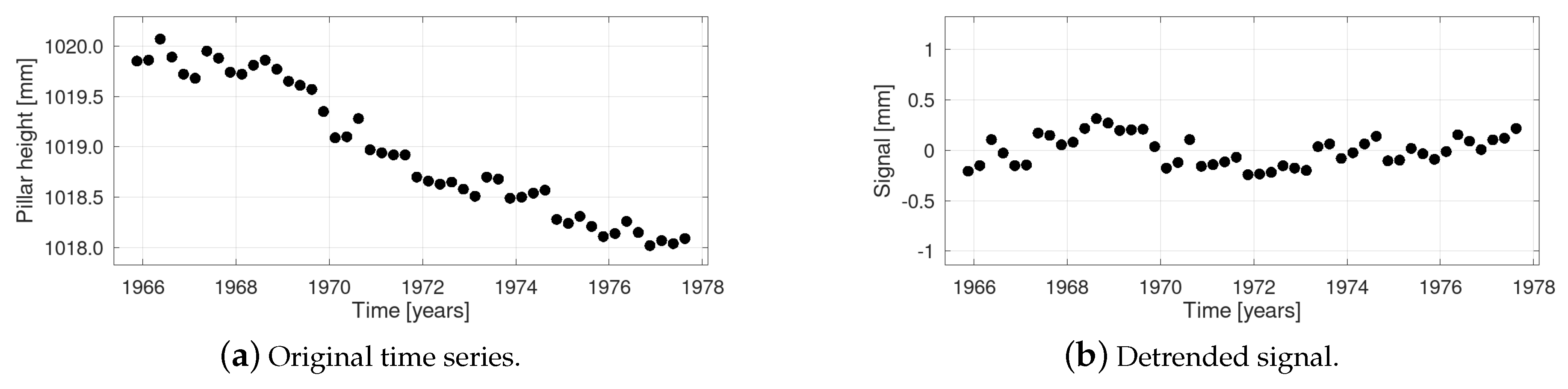
7. An Example: Milan Cathedral Deformation Time Series

This example is the well known deformation time series of Milan Cathedral [62]. The time series measurements are levelling heights of a pillar in the period of 1965 to 1977. It is an equidistant time series having 48 values with sampling interval $\Delta t=0.25$ years. In [62], the time series is deseasonalized and then used for further analysis with autoregressive processes. In this paper, a consistent modeling of the whole signal component without deseasonalization is seen to be advantageous. The time series is detrended using a linear function and the remaining residuals define the stochastic signal, cf. Figure 1.

Based on the detrended time series, the biased estimator is used to determine the empirical covariances in all examples. The order for the AR(p)-process is chosen as $p=4$. Four different covariance functions were determined based on the method proposed here. All second-order components of the estimated covariance functions are converted to the SOGM parametrization and individually tested for positive semi-definiteness using Equation (8).

As a kind of reference, a manual approach (cf. Figure 2a) was chosen. A single SOGM is adjusted by manually tuning the parameters to achieve a good fit for all empirical covariances, ignoring ${\tilde{g}}_0^{\Delta \mathcal{L}}$. This function follows the long-wavelength oscillation contained in the signal.

In a second approach, the process coefficients are estimated using the YW-Equations (14b) with the covariances ${\tilde{g}}_0^{\Delta \mathcal{L}}$ to ${\tilde{g}}_p^{\Delta \mathcal{L}}$. Furthermore, the system in Equation (28) is solved uniquely using the lags from ${\tilde{g}}_1^{\Delta \mathcal{L}}$ up to ${\tilde{g}}_m^{\Delta \mathcal{L}}$ with $m=p$. In Figure 2b, the covariance function exactly interpolates the first five values. This covariance model with relatively low order already contains a second high-frequent oscillation of a 1-year period, caused by annual temperature variations, which is not obvious at first. However, the function misses the long wavelength oscillation and does not fit well to the higher covariances. Here, the model order can of course be increased in order to interpolate more covariances. However, it will be demonstrated now that the covariance structure at hand can in fact also be modeled with the low-order AR(4)-model.

For the remaining examples, the process coefficients are estimated using the MYW-Equations (14c) with $n=24$ covariances. As a first case, the function was estimated with a manually chosen nugget effect, i.e., ${\tilde{g}}_0^{\mathcal{S}}={\tilde{g}}_0^{\Delta \mathcal{L}}-0.0019$, and by solving Equation (28) with $m=p-1$, which results in a pure AR(4)-process. The covariance function represented by Figure 2c approximates the correlations better compared to first two cases. The shape models all oscillations, but does not exactly pass through all values at the lags $\tau =1.5$ to $4$ years.

Finally, the system of Equation (28) was solved using the higher lags ${\tilde{g}}_m^{\mathcal{S}}$ up to $m=14$ in order to enforce an ARMA-model. However, the best fit exceeds ${\tilde{g}}_0^{\Delta \mathcal{L}}$, such that the best valid fit is achieved with a no nugget effect in the signal covariance model and a covariance function exactly interpolating ${\tilde{g}}_0^{\Delta \mathcal{L}}$. Thus, we fix $g^{\mathcal{S}}\left(0\right)$ to ${\tilde{g}}_0^{\Delta \mathcal{L}}$ using a constrained least squares adjustment, which is the result shown here. In comparison, Figure 2d shows the most flexible covariance function. The function passes very close to nearly all covariances up to $\tau =6$ years and the fit is still good beyond that. The approximated ARMA-process with order $p=4$ allows more variation of the covariance function and the function fits better to higher lags.

The corresponding process parameters for the last two examples are listed in

Table 2. Approximation with pure AR(2)-components. The frequency is also given as ordinary frequency ${\nu }_0$. The variance of the combined covariance function amounts to ${\sigma }^2=0.02046\mathrm{m}{\mathrm{m}}^2$ which leads to ${\sigma }_{\mathcal{N}}=0.04359\mathrm{m}\mathrm{m}$. ${\omega }_0$ and $\eta$ are given in units of radians.

	Roots	Frequency ${\mathit{\omega }}_0$	Frequency ${\mathit{\nu }}_0$	Damping $\mathit{\zeta }$	Phase $\mathit{\eta }$	$\mathit{\alpha }=arcsin\left(\mathit{\zeta }\right)$
A	$\phantom{-}0.91262+0.18022i$	$0.20794$	$0.13238$ [1/year]	$0.34774$	$-0.15819$	$0.35516$
	$\phantom{-}0.91262-0.18022i$
B	$0.0042636+0.93678i$	$1.5676$	$0.99797$ [1/year]	$0.041655$	$0.040221$	$0.041667$
	$0.0042636-0.93678i$

and

Table 3. Approximation with SOGM-components, i.e., ARMA(2,q)-models. The variance of the combined covariance function amounts to ${\sigma }^2=0.02235\mathrm{m}{\mathrm{m}}^2$.

	Roots	Frequency ${\mathit{\omega }}_0$	Frequency ${\mathit{\nu }}_0$	Damping $\mathit{\zeta }$	Phase $\mathit{\eta }$	$\mathit{\alpha }=arcsin\left(\mathit{\zeta }\right)$
A	$\phantom{-}0.91262+0.18022i$	$0.20794$	$0.13238$ [1/year]	$0.34774$	$-0.30670$	$0.35516$
	$\phantom{-}0.91262-0.18022i$
B	$0.0042636+0.93678i$	$1.5676$	$0.99797$ [1/year]	$0.041655$	$0.026133$	$0.041667$
	$0.0042636-0.93678i$

. All parameters are given with numbers in rational approximation. The positive definiteness is directly visible by the condition $\left|\eta \right|\le \alpha$. The approximated pure AR(4)-process in Table 2 is relatively close to being invalid for the second component but still within the limits. For the ARMA-model, notably, poles, frequency, and attenuation parameters are the same, cf. Table 3. Just the phases $\eta$ of the two components are different and also inside the bounds of positive definiteness. The resulting covariance function using the ARMA-model (Figure 2d) is given by

$$\begin{array}{c}\hfill \begin{array}{cc}\hfill g^{\mathcal{S}}\left(\tau \right)=& 0.01680·{\mathrm{e}}^{-0.0723\frac{\tau }{\Delta t}}\left(cos\left(0.1950\frac{\tau }{\Delta t}\right)-0.3167sin\left(0.1950\frac{\tau }{\Delta t}\right)\right)+\hfill \\ \hfill & \begin{array}{c}\hfill 0.00555·{\mathrm{e}}^{-0.0653\frac{\tau }{\Delta t}}\left(cos\left(1.5662\frac{\tau }{\Delta t}\right)+0.02614sin\left(1.5662\frac{\tau }{\Delta t}\right)\right)\end{array}\hfill \\ \hfill & \hfill \mathrm{with}\tau \mathrm{in}\mathrm{years}.\end{array}\end{array}$$

(30)

It needs to be noted here that the connection of unitless poles and parameters with distance $\tau$ cannot be done in the way indicated by Section 2, Section 3, Section 4, Section 5 and Section 6. In fact, for the correct covariance function, the argument $\tau$ requires a scaling with sampling interval $\Delta t$ which was omitted for reasons of brevity and comprehensibility. As a consequence, the scaling $1/\Delta t$ to the argument $\tau$ is included in Equation (30). We also assess the same factor to the transition from ${\omega }_0$ to ordinary frequency ${\nu }_0$ given in Table 2 and Table 3.

Using the process characteristics in Table 2 and Table 3, it is obvious now that the long wavelength oscillation has a period of about $7.6$ years. Diagnostics of the estimated process can be done in the same way in order to possibly discard certain components if they are irrelevant. In summary, the proposed approach can realize a much better combined modeling of long and short-wavelength signal components without manual choices of frequencies, amplitudes, and phases. The modified Yule–Walker equations prove valuable for a good fit of the covariance function due to the stabilization by higher lags. ARMA-models provide a further enhanced flexibility of the covariance function.

8. Summary and Conclusions

In this paper, we presented an estimation procedure for covariance functions based on methodology of stochastic processes and a simple and straightforward numerical method. The approach is based on the analogy of the covariance functions defined by the SOGM-process and autoregressive processes. Thus, we provide the most general damped oscillating autocorrelation function built from exponential and trigonometric terms, which includes several simple analytical covariance models as limit cases.

The covariance models of autoregressive process as well as of ARMA-processes correspond to a linear combination of covariance functions of second-order Gauss–Markov (SOGM) processes. We provide fitting procedures of these covariance functions to empirical covariance estimates based on simple systems of linear equations. Notably, the numerical method easily extends to ARMA-processes with the same linear system of equations. In the future, research will be done towards possibilities of constraining the bounds of stationarity and positive definiteness in the estimation steps.

The great advantage is that the method is automated and gives the complete model instead of needing to manually model each component. Our method is very flexible because the process estimation automatically chooses complex or real poles, depending on whether more oscillating or only decaying covariance components are necessary to model the process. Naturally, our approach restricts to stationary time series. In non-stationary cases, the empirically estimated covariance sequence would not decrease with increasing lag and by this contradict the specifications of covariance functions, e.g., ${\tilde{g}}_0^{\Delta \mathcal{L}}$ being the largest covariance, see Section 2 and [28]. Such an ill-shaped covariance sequence will definitely result in non-stationary autoregressive poles and the method will fail.

The real world example has shown that covariance function estimation can in fact give good fitting results even for complex covariance structures. The guidelines presented here provide multiple possibilities for fitting procedures and process diagnostics. As a result, covariance function estimation is greatly automatized with a generic method and a more consistent approach to a complete signal modeling is provided.

References

1. Kolmogorov, A.N. Grundbegriffe der Wahrscheinlichkeitsrechnung; Springer: Berlin/Heidelberg, Germany, 1933. [Google Scholar] [CrossRef]
2. Wiener, N. Extrapolation, Interpolation, and Smoothing of Stationary Time Series; MIT Press: Cambridge, MA, USA, 1949. [Google Scholar]
3. Moritz, H. Advanced Least-Squares Methods; Number 175 in Reports of the Department of Geodetic Science; Ohio State University Research Foundation: Columbus, OH, USA, 1972. [Google Scholar]
4. Moritz, H. Advanced Physical Geodesy; Wichmann: Karlsruhe, Germany, 1980. [Google Scholar]
5. Schuh, W.D. Signalverarbeitung in der Physikalischen Geodäsie. In Handbuch der Geodäsie, Erdmessung und Satellitengeodäsie; Freeden, W., Rummel, R., Eds.; Springer Reference Naturwissenschaften; Springer: Berlin/Heidelberg, Germany, 2016; pp. 73–121. [Google Scholar] [CrossRef]
6. Moritz, H. Least-Squares Collocation; Number 75 in Reihe A; Deutsche Geodätische Kommission: München, Germany, 1973. [Google Scholar]
7. Reguzzoni, M.; Sansó, F.; Venuti, G. The Theory of General Kriging, with Applications to the Determination of a Local Geoid. Geophys. J. Int. 2005, 162, 303–314. [Google Scholar] [CrossRef] [Green Version]
8. Moritz, H. Covariance Functions in Least-Squares Collocation; Number 240 in Reports of the Department of Geodetic Science; Ohio State University: Columbus, OH, USA, 1976. [Google Scholar]
9. Cressie, N.A.C. Statistics for Spatial Data; Wiley Series in Probability and Statistics; Wiley: New York, NY, USA, 1991. [Google Scholar] [CrossRef]
10. Chilès, J.P.; Delfiner, P. Geostatistics: Modeling Spatial Uncertainty; Wiley Series in Probability and Statistics; John Wiley & Sons: Hoboken, NJ, USA, 1999. [Google Scholar] [CrossRef]
11. Thiébaux, H.J. Anisotropic Correlation Functions for Objective Analysis. Mon. Weather Rev. 1976, 104, 994–1002. [Google Scholar] [CrossRef] [Green Version]
12. Franke, R.H. Covariance Functions for Statistical Interpolation; Technical Report NPS-53-86-007; Naval Postgraduate School: Monterey, CA, USA, 1986. [Google Scholar]
13. Gneiting, T. Correlation Functions for Atmospheric Data Analysis. Q. J. R. Meteorol. Soc. 1999, 125, 2449–2464. [Google Scholar] [CrossRef]
14. Gneiting, T.; Kleiber, W.; Schlather, M. Matérn Cross-Covariance Functions for Multivariate Random Fields. J. Am. Stat. Assoc. 2010, 105, 1167–1177. [Google Scholar] [CrossRef]
15. Meissl, P. A Study of Covariance Functions Related to the Earth’s Disturbing Potential; Number 151 in Reports of the Department of Geodetic Science; Ohio State University: Columbus, OH, USA, 1971. [Google Scholar]
16. Tscherning, C.C.; Rapp, R.H. Closed Covariance Expressions for Gravity Anomalies, Geoid Undulations, and Deflections of the Vertical Implied by Anomaly Degree Variance Models; Technical Report DGS-208; Ohio State University, Department of Geodetic Science: Columbus, OH, USA, 1974. [Google Scholar]
17. Mussio, L. Il metodo della collocazione minimi quadrati e le sue applicazioni per l’analisi statistica dei risultati delle compensazioni. In Ricerche Di Geodesia, Topografia e Fotogrammetria; CLUP: Milano, Italy, 1984; Volume 4, pp. 305–338. [Google Scholar]
18. Koch, K.R.; Kuhlmann, H.; Schuh, W.D. Approximating Covariance Matrices Estimated in Multivariate Models by Estimated Auto- and Cross-Covariances. J. Geod. 2010, 84, 383–397. [Google Scholar] [CrossRef]
19. Sansò, F.; Schuh, W.D. Finite Covariance Functions. Bull. Géodésique 1987, 61, 331–347. [Google Scholar] [CrossRef]
20. Gaspari, G.; Cohn, S.E. Construction of Correlation Functions in Two and Three Dimensions. Q. J. R. Meteorol. Soc. 1999, 125, 723–757. [Google Scholar] [CrossRef]
21. Gneiting, T. Compactly Supported Correlation Functions. J. Multivar. Anal. 2002, 83, 493–508. [Google Scholar] [CrossRef] [Green Version]
22. Kraiger, G. Untersuchungen zur Prädiktion nach kleinsten Quadraten mittels empirischer Kovarianzfunktionen unter besonderer Beachtung des Krümmungsparameters; Number 53 in Mitteilungen der Geodätischen Institute der Technischen Universität Graz; Geodätische Institute der Technischen Universität Graz: Graz, Austria, 1987. [Google Scholar]
23. Jenkins, G.M.; Watts, D.G. Spectral Analysis and Its Applications; Holden-Day: San Francisco, CA, USA, 1968. [Google Scholar]
24. Box, G.; Jenkins, G. Time Series Analysis: Forecasting and Control; Series in Time Series Analysis; Holden-Day: San Francisco, CA, USA, 1970. [Google Scholar]
25. Maybeck, P.S. Stochastic Models, Estimation, and Control; Vol. 141-1, Mathematics in Science and Engineering; Academic Press: New York, NY, USA, 1979. [Google Scholar] [CrossRef]
26. Priestley, M.B. Spectral Analysis and Time Series; Academic Press: London, UK; New York, NY, USA, 1981. [Google Scholar]
27. Yaglom, A.M. Correlation Theory of Stationary and Related Random Functions: Volume I: Basic Results; Springer Series in Statistics; Springer: New York, NY, USA, 1987. [Google Scholar]
28. Brockwell, P.J.; Davis, R.A. Time Series Theory and Methods, 2nd ed.; Springer Series in Statistics; Springer: New York, NY, USA, 1991. [Google Scholar] [CrossRef]
29. Hamilton, J.D. Time Series Analysis; Princeton University Press: Princeton, NJ, USA, 1994. [Google Scholar]
30. Buttkus, B. Spectral Analysis and Filter Theory in Applied Geophysics; Springer: Berlin/Heidelberg, Germany, 2000. [Google Scholar] [CrossRef]
31. Jones, R.H. Fitting a Continuous Time Autoregression to Discrete Data. In Applied Time Series Analysis II; Findley, D.F., Ed.; Academic Press: New York, NY, USA, 1981; pp. 651–682. [Google Scholar] [CrossRef]
32. Jones, R.H.; Vecchia, A.V. Fitting Continuous ARMA Models to Unequally Spaced Spatial Data. J. Am. Stat. Assoc. 1993, 88, 947–954. [Google Scholar] [CrossRef]
33. Brockwell, P.J. Continuous-Time ARMA Processes. In Stochastic Processes: Theory and Methods; Shanbhag, D., Rao, C., Eds.; Volume 19, Handbook of Statistics; North-Holland: Amsterdam, The Netherlands, 2001; pp. 249–276. [Google Scholar] [CrossRef]
34. Kelly, B.C.; Becker, A.C.; Sobolewska, M.; Siemiginowska, A.; Uttley, P. Flexible and Scalable Methods for Quantifying Stochastic Variability in the Era of Massive Time-Domain Astronomical Data Sets. Astrophys. J. 2014, 788, 33. [Google Scholar] [CrossRef] [Green Version]
35. Tómasson, H. Some Computational Aspects of Gaussian CARMA Modelling. Stat. Comput. 2015, 25, 375–387. [Google Scholar] [CrossRef] [Green Version]
36. Schuh, W.D. Tailored Numerical Solution Strategies for the Global Determination of the Earth’s Gravity Field; Volume 81, Mitteilungen der Geodätischen Institute; Technische Universität Graz (TUG): Graz, Austria, 1996. [Google Scholar]
37. Schuh, W.D. The Processing of Band-Limited Measurements; Filtering Techniques in the Least Squares Context and in the Presence of Data Gaps. Space Sci. Rev. 2003, 108, 67–78. [Google Scholar] [CrossRef]
38. Klees, R.; Ditmar, P.; Broersen, P. How to Handle Colored Observation Noise in Large Least-Squares Problems. J. Geod. 2003, 76, 629–640. [Google Scholar] [CrossRef] [Green Version]
39. Siemes, C. Digital Filtering Algorithms for Decorrelation within Large Least Squares Problems. Ph.D. Thesis, Landwirtschaftliche Fakultät der Universität Bonn, Bonn, Germany, 2008. [Google Scholar]
40. Krasbutter, I.; Brockmann, J.M.; Kargoll, B.; Schuh, W.D. Adjustment of Digital Filters for Decorrelation of GOCE SGG Data. In Observation of the System Earth from Space—CHAMP, GRACE, GOCE and Future Missions; Flechtner, F., Sneeuw, N., Schuh, W.D., Eds.; Vol. 20, Advanced Technologies in Earth Sciences, Geotechnologien Science Report; Springer: Berlin/Heidelberg, Germany, 2014; pp. 109–114. [Google Scholar] [CrossRef]
41. Farahani, H.H.; Slobbe, D.C.; Klees, R.; Seitz, K. Impact of Accounting for Coloured Noise in Radar Altimetry Data on a Regional Quasi-Geoid Model. J. Geod. 2017, 91, 97–112. [Google Scholar] [CrossRef] [Green Version]
42. Schuh, W.D.; Brockmann, J.M. The Numerical Treatment of Covariance Stationary Processes in Least Squares Collocation. In Handbuch der Geodäsie: 6 Bände; Freeden, W., Rummel, R., Eds.; Springer Reference Naturwissenschaften; Springer: Berlin/Heidelberg, Germany, 2018; pp. 1–36. [Google Scholar] [CrossRef]
43. Pail, R.; Bruinsma, S.; Migliaccio, F.; Förste, C.; Goiginger, H.; Schuh, W.D.; Höck, E.; Reguzzoni, M.; Brockmann, J.M.; Abrikosov, O.; et al. First, GOCE Gravity Field Models Derived by Three Different Approaches. J. Geod. 2011, 85, 819. [Google Scholar] [CrossRef] [Green Version]
44. Brockmann, J.M.; Zehentner, N.; Höck, E.; Pail, R.; Loth, I.; Mayer-Gürr, T.; Schuh, W.D. EGM_TIM_RL05: An Independent Geoid with Centimeter Accuracy Purely Based on the GOCE Mission. Geophys. Res. Lett. 2014, 41, 8089–8099. [Google Scholar] [CrossRef]
45. Schubert, T.; Brockmann, J.M.; Schuh, W.D. Identification of Suspicious Data for Robust Estimation of Stochastic Processes. In IX Hotine-Marussi Symposium on Mathematical Geodesy; Sneeuw, N., Novák, P., Crespi, M., Sansò, F., Eds.; International Association of Geodesy Symposia; Springer: Berlin/ Heidelberg, Germany, 2019. [Google Scholar] [CrossRef]
46. Krarup, T. A Contribution to the Mathematical Foundation of Physical Geodesy; Number 44 in Meddelelse; Danish Geodetic Institute: Copenhagen, Denmark, 1969. [Google Scholar]
47. Amiri-Simkooei, A.; Tiberius, C.; Teunissen, P. Noise Characteristics in High Precision GPS Positioning. In VI Hotine-Marussi Symposium on Theoretical and Computational Geodesy; Xu, P., Liu, J., Dermanis, A., Eds.; International Association of Geodesy Symposia; Springer: Berlin/ Heidelberg, Germany, 2008; pp. 280–286. [Google Scholar] [CrossRef] [Green Version]
48. Kermarrec, G.; Schön, S. On the Matérn Covariance Family: A Proposal for Modeling Temporal Correlations Based on Turbulence Theory. J. Geod. 2014, 88, 1061–1079. [Google Scholar] [CrossRef]
49. Tscherning, C.; Knudsen, P.; Forsberg, R. Description of the GRAVSOFT Package; Technical Report; Geophysical Institute, University of Copenhagen: Copenhagen, Denmark, 1994. [Google Scholar]
50. Arabelos, D.; Tscherning, C.C. Globally Covering A-Priori Regional Gravity Covariance Models. Adv. Geosci. 2003, 1, 143–147. [Google Scholar] [CrossRef] [Green Version]
51. Arabelos, D.N.; Forsberg, R.; Tscherning, C.C. On the a Priori Estimation of Collocation Error Covariance Functions: A Feasibility Study. Geophys. J. Int. 2007, 170, 527–533. [Google Scholar] [CrossRef] [Green Version]
52. Darbeheshti, N.; Featherstone, W.E. Non-Stationary Covariance Function Modelling in 2D Least-Squares Collocation. J. Geod. 2009, 83, 495–508. [Google Scholar] [CrossRef] [Green Version]
53. Barzaghi, R.; Borghi, A.; Sona, G. New Covariance Models for Local Applications of Collocation. In IV Hotine-Marussi Symposium on Mathematical Geodesy; Benciolini, B., Ed.; International Association of Geodesy Symposia; Springer: Berlin/Heidelberg, Germany, 2001; pp. 91–101. [Google Scholar] [CrossRef] [Green Version]
54. Kvas, A.; Behzadpour, S.; Ellmer, M.; Klinger, B.; Strasser, S.; Zehentner, N.; Mayer-Gürr, T. ITSG-Grace2018: Overview and Evaluation of a New GRACE-Only Gravity Field Time Series. J. Geophys. Res. Solid Earth 2019, 124, 9332–9344. [Google Scholar] [CrossRef] [Green Version]
55. Rasmussen, C.; Williams, C. Gaussian Processes for Machine Learning; Adaptive Computation and Machine Learning; MIT Press: Cambridge, MA, USA, 2006. [Google Scholar]
56. Jarmołowski, W.; Bakuła, M. Precise Estimation of Covariance Parameters in Least-Squares Collocation by Restricted Maximum Likelihood. Studia Geophysica et Geodaetica 2014, 58, 171–189. [Google Scholar] [CrossRef]
57. Fitzgerald, R.J. Filtering Horizon-Sensor Measurements for Orbital Navigation. J. Spacecr. Rocket. 1967, 4, 428–435. [Google Scholar] [CrossRef]
58. Jackson, L.B. Digital Filters and Signal Processing, 3rd ed.; Springer: New York, NY, USA, 1996. [Google Scholar] [CrossRef]
59. Titov, O.A. Estimation of the Subdiurnal UT1-UTC Variations by the Least Squares Collocation Method. Astron. Astrophys. Trans. 2000, 18, 779–792. [Google Scholar] [CrossRef]
60. Halsig, S. Atmospheric Refraction and Turbulence in VLBI Data Analysis. Ph.D. Thesis, Landwirtschaftliche Fakultät der Universität Bonn, Bonn, Germany, 2018. [Google Scholar]
61. Bochner, S. Lectures on Fourier Integrals; Number 42 in Annals of Mathematics Studies; Princeton University Press: Princeton, NJ, USA, 1959. [Google Scholar]
62. Sansò, F. The Analysis of Time Series with Applications to Geodetic Control Problems. In Optimization and Design of Geodetic Networks; Grafarend, E.W., Sansò, F., Eds.; Springer: Berlin/Heidelberg, Germany, 1985; pp. 436–525. [Google Scholar] [CrossRef]
63. Kay, S.; Marple, S. Spectrum Analysis—A Modern Perspective. Proc. IEEE 1981, 69, 1380–1419. [Google Scholar] [CrossRef]
64. Friedlander, B.; Porat, B. The Modified Yule-Walker Method of ARMA Spectral Estimation. IEEE Trans. Aerosp. Electron. Syst. 1984, AES-20, 158–173. [Google Scholar] [CrossRef]
65. Gelb, A. Applied Optimal Estimation; The MIT Press: Cambridge, MA, USA, 1974. [Google Scholar]
66. Phadke, M.S.; Wu, S.M. Modeling of Continuous Stochastic Processes from Discrete Observations with Application to Sunspots Data. J. Am. Stat. Assoc. 1974, 69, 325–329. [Google Scholar] [CrossRef]
67. Tunnicliffe Wilson, G. Some Efficient Computational Procedures for High Order ARMA Models. J. Stat. Comput. Simul. 1979, 8, 301–309. [Google Scholar] [CrossRef]
68. Woodward, W.A.; Gray, H.L.; Haney, J.R.; Elliott, A.C. Examining Factors to Better Understand Autoregressive Models. Am. Stat. 2009, 63, 335–342. [Google Scholar] [CrossRef]
69. Koch, K.R. Parameter Estimation and Hypothesis Testing in Linear Models, 2nd ed.; Springer: Berlin/Heidelberg, Germany, 1999. [Google Scholar] [CrossRef]
70. Roese-Koerner, L. Convex Optimization for Inequality Constrained Adjustment Problems. Ph.D. Thesis, Landwirtschaftliche Fakultät der Universität Bonn, Bonn, Germany, 2015. [Google Scholar]
Figure 1. Milan Cathedral time series.
Mathematics 08 00591 g001
Figure 2. Covariance functions for the Milan Cathedral data sets determined with four different approaches: (a) Intuitive ("naive") approach using a single SOGM-process with manually adjusted parameters. (b) Covariance function resulting from the interpolation of the first p + 1 covariances with a pure AR(4)-processes. (c) Covariance function resulting from an approximation procedure of g ˜ 0 S to g ˜ 24 S using a pure AR-process with p = 4 . (d) Covariance function based on approximation with the most flexible ARMA-process ( p = 4 ). Empirical covariances are shown by the black dots. The variances g ˜ 0 S of the covariance functions are indicated by circles. The parameters of the processes (c,d) are provided in Table 2 and Table 3.
Mathematics 08 00591 g002