1. Introduction
A digital filter is a hardware or software used to reduce the noise in the data of a system, extract information, or predict and rebuild the behavior of a system [
1]. In [
1,
2], two basic areas in digital filtering theory are presented: estimation and identification. Depending on the time evolution interval
k, in which the digital filter works, three filter actions are defined: reconstruction, filtering and prediction.
A Real-time System (RTS) interacts with a known dynamic environment, during a certain instant of occurrence
μk of the physical world, and the system output depends on the input through a processing intrinsic time ε [
3], and it must be completed into a sampling time of the dynamic process [
4]. The interaction between RTS and dynamic processes takes place through the detection of the system variables with the use of transducers like semiconductor devices. The sensed signals may be affected by internal and external noise causing measurement errors. Filtering techniques can be added in the RTS, integrating an architecture that can be used in industrial processes interactions, according to [
5,
6]. One of the most widely used dynamic filters that performs estimation and identification is the Kalman filter (KF); its digital version is described as an adaptive iterative algorithm designed to identify the state vector of state space linear systems. The real-time implementation of this filter requires an analysis of the time constraints imposed by the system. The correct characterization of these restrictions in addition with the recursive form of the algorithm enable the real-time simulation.
In the last decades, the application of gas turbines has demonstrated a significant growth [
7]. These engines are principal drivers for electricity production and are widely used in oil platforms, chemical plants, gas stations, and so on. Air transport is another large area of application, where a turbofan is a main engine type. Being relatively light and compact, aircraft gas turbine engines provide high power and efficiency. To have the best performances, the engine must operate near its limits at all operating modes. To this end, an engine control must be accurate. The enhancement of an engine control system makes control laws more complex, and mathematical modeling becomes increasingly useful in the development of such a system [
8]. Under contradictive demands of high engine performances, reliability, safety, and low maintenance costs, the use of developed diagnostic systems becomes an effective strategy. The development and operation of these systems are also based on different mathematical models [
9,
10]. Nonlinear dynamic physics-based engine models are too complex and slow to be used in on-board control and diagnostic systems. Instead, linear dynamic models and Kalman filtering operating in real time are widespread [
8,
9].
In this paper, a real-time implementation on a Single Board Computer (SBC) of a Kalman digital filter applied to the hybrid dynamic model of a turbofan engine is proposed. The objective is to closely examine a real-time operation of the filter. The execution time is verified at each time instance and under the conditions of a specialized computer similar to an engine control processor. This examination allows us to draw a sound conclusion whether the filter and model can be implemented in real on-board engine and aircraft systems. To our knowledge, such a strict verification is novel.
The mathematical model corresponds to a linear discrete time stochastic dynamic system expressed in a state-space form. For the experimental results, a Raspberry Pi 2 Model B® was used. This computer has a quad-core ARM Cortex-A7 CPU at 900 MHz, graphics processor Video-Core IV and 1 GB RAM. A strong contribution is a real-time implementation details of the digital Kalman filter; including the development of a library in C language for RT-Raspbian®.
The rest of this paper is organized as follows.
Section 2 presents the gas turbine engine models.
Section 3 shows the hybrid dynamic model for a gas turbine. In
Section 4, a real-time simulation of a gas turbine engine is introduced.
Section 5 presents the state vector identification using an embedded version of the Kalman filter. In
Section 6, a real-time response analysis is presented. Finally, the conclusions are provided.
3. Hybrid Dynamic Model
To obtain dynamic values of gas path variables in a simplified hybrid dynamic model, the dynamic corrections of Equations (5) and (6) are added to the static model values:
Table 1 specifies the control, state space, and monitored variables. The simulation was performed at standard ambient conditions, therefore, the static and the linear dynamic models have only one operating condition that is the control variable (power set). A pressure ratio is chosen as a static control variable
us, and a fuel flow is a dynamic control variable
u.
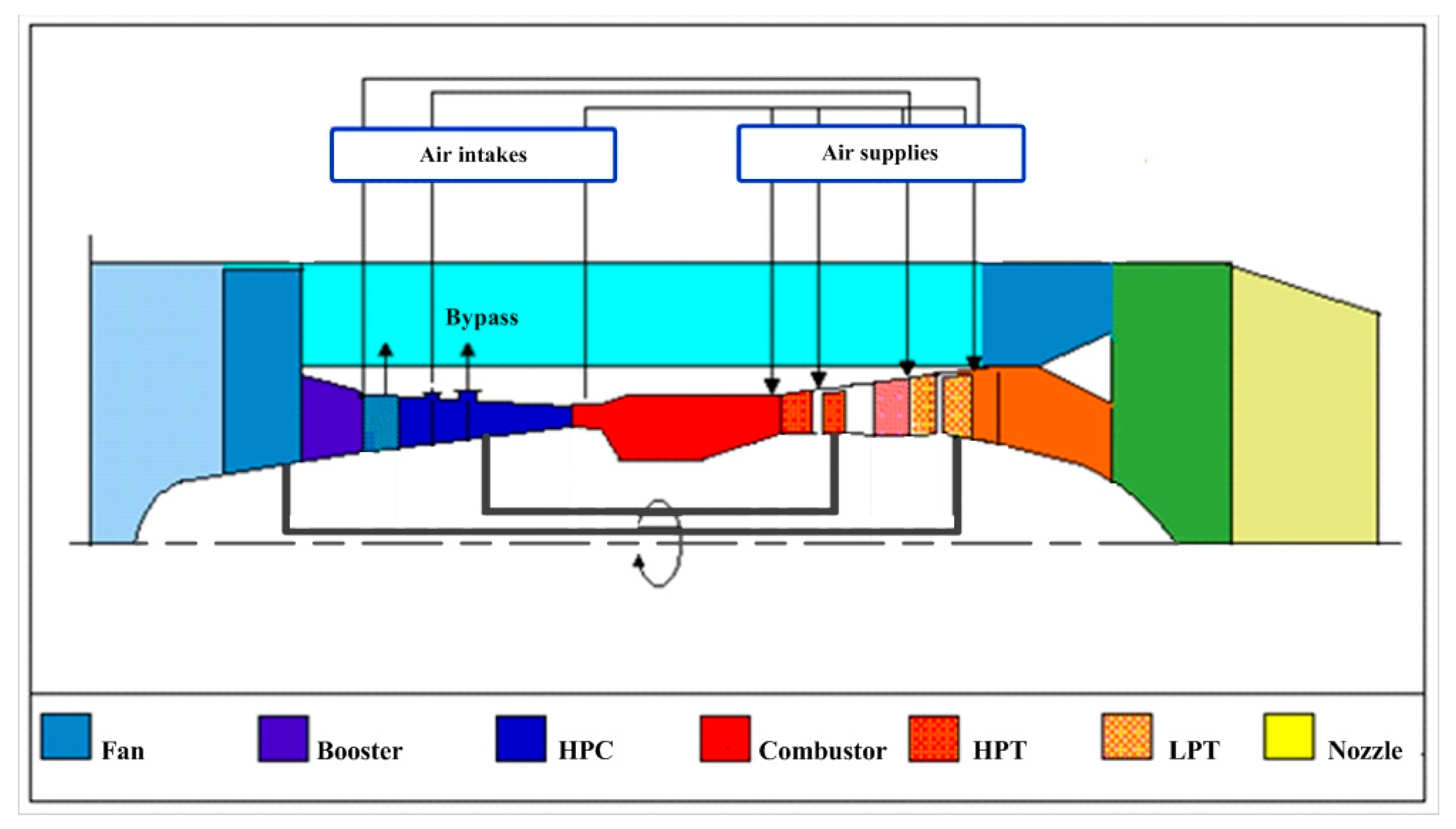
The static performance depends on the power level; a piecewise approximation is used to determine the unknown values in Equations (3), (5), and (6). According to the control variable (power set),
, the interval of engine operation is divided into five zones
iz = 1, 2…5, where the last zone corresponds to the highest power. This division is related to the action of bypass valves, which causes the shifts of engine performances. These zones are also the result of the trade-off between approximation accuracy and simplicity. The static quantities
ust,
Xst, and
Yst are presented as polynomial functions of the variable
. The matrixes
A,
B,
C, and
D are computed using the static nonlinear model, see Equation (1). In total, the approximation can be given by the system:
Variables are computed for times t = t1, t2, t3, … tk, tk+1, … tn, determined with a constant time interval Δt = tk+1 − tk. The transient is set according to a control variable time profile . The simulation is defined in 10 steps:
Step 1. Current time
is given by:
Step 2. Using a time profile
, the dynamic control variable is determined by:
Step 3. The static control variable is known from the previous time point k−1.
Step 4. According to Equation (10), the zone number is obtained:
Step 5. Equation (11) is given by the following static values:
Step 6. The differences are calculated according to:
The dynamic and static values are calculated. Note that the state space variable dynamic values are known from the previous instant k − 1.
Step 7. According to Equation (12), the following matrices are chosen:
Step 8. Placing the matrixes of Equation (18) in (5), the state space derivatives are determined by:
and the changes of monitored variables are defined according to:
Step 9. The knowledge of the derivatives allows us to compute dynamic values of state space variables for the next point
k + 1.
Step 10. Dynamic values of monitored variables are calculated as:
The first monitored variable is the pressure
PHPC, and its value
is used for the next time to calculate
as a static control variable
. Therefore, for each iteration
k and time
tk, the 10 steps described above are executed to determine the dynamic control variable
and the dynamic values
. The iteration
k also provides the values
X(
k + 1) and
used as input data in the next iteration. In this way, continuous dynamic gas turbine simulation in the interval (
−
) is achieved. The scheme in
Figure 2 illustrates this simulation.
4. Real-Time Simulation of GTE
The hybrid model was programmed in the SBC Raspberry pi 2 model B
® with RT-Raspbian and C language, [
17]; some libraries have been developed to provide necessary tools for (a) the use of matrices and vectors, (b) dynamic memory management, (c) simulation of state-space systems, and (d) approximation of systems by equations in matrix finite differences. The gas turbine engine operation was simulated during 10 s with a time step
, resulting in 200 real-time instances. The fuel consumption was linearly increased from an idle regime value at
t = 1 s to a take-off regime value at
t = 2 s. The resulting time plots of static and dynamic values of the variables and dynamic changes can be seen in
Figure 3,
Figure 4 and
Figure 5.
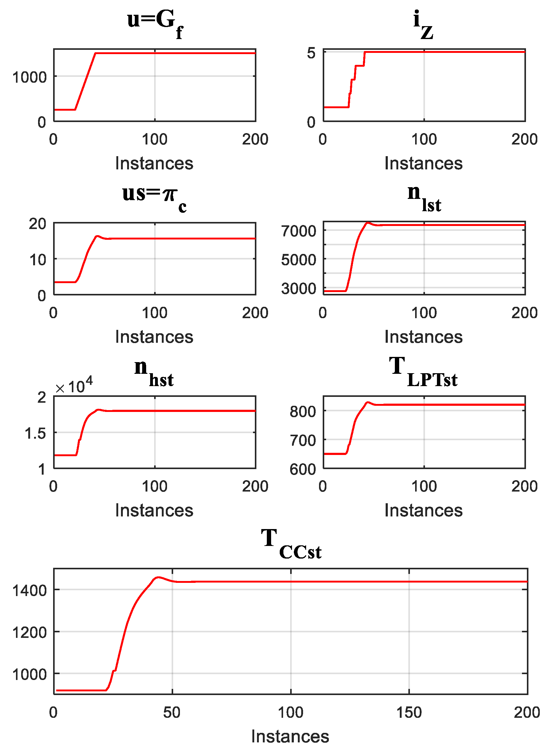
In
Figure 3, the plot
u =
Gf(
k) shows the lineal behavior of the control variable. The fuel consumption increases, causing the increment in the zone number, as is shown in plot
iz(
k).
The control variable
us is set as a dynamic value of
from the previous instance, therefore,
us changes dynamically after the instance 40 generating a transient response. In Equation (10), the static variables
Xst and
Yst depend on
, therefore, their behavior should be similar to
. This is shown in
Figure 3 with the plots of
nlst,
nhst,
PHPCst,
TLPTst, and
TCCst.
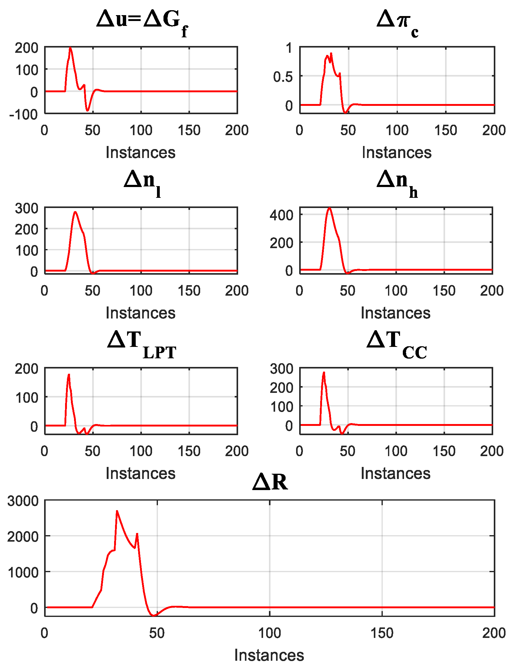
To verify the dynamic behavior of the simulated engine, the plots of the dynamic deviations (changes) are presented in
Figure 4. The overshoots that appear at the point
t = 1 s (instance 20) are greater than the ones after
t = 2 s (instance 40), then stabilize approximately at the point
t = 3 s (instance 60).
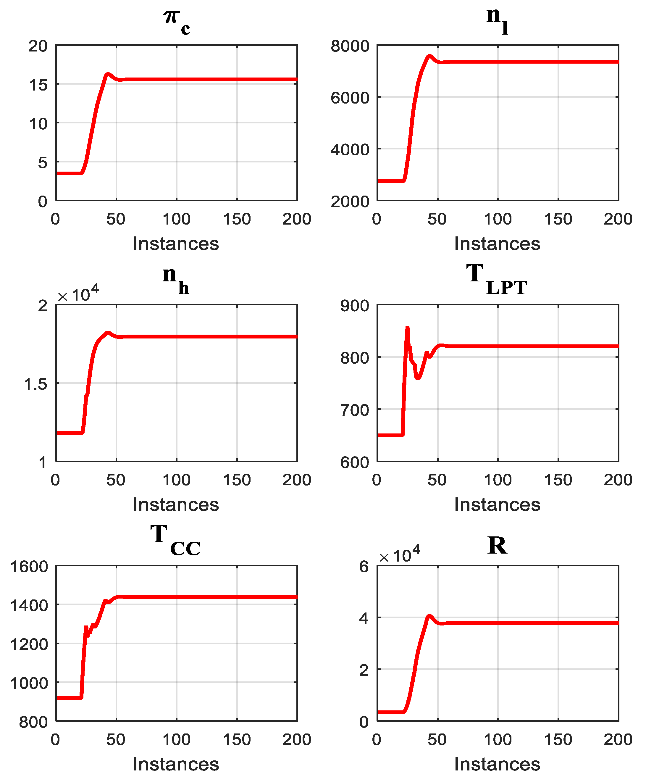
Figure 5 integrates the static values and dynamic deviations resulting in dynamic values of gas turbine variables. These dynamic values were compared with the outputs of the dynamic nonlinear model, Equation (2), and its accuracy was confirmed. Thus,
Figure 3,
Figure 4 and
Figure 5 validate the hybrid model.
5. State Vector Identification by Kalman Filter
The hybrid model described in
Section 3 and the variables simulated with this model in
Section 4 do not consider internal or external noise. Since in a real system (gas turbine), the measurements contain noise, the computed variables will have errors. To reduce this noise and minimize the random estimation errors, a Kalman filter is used. The Digital Kalman filter is an iterative algorithm based on a linear state space model of a non-deterministic system in which internal noise
V(
k) and external noise
W(
k) have been added in Equations (5) and (6) respectively [
18]. The noise interacts with the system and modifies it, resulting in a stochastic process. The filter is applied to the systems to identify its state vector and then reconstruct its outputs with minimum errors. In other cases, the Kalman filter is applied to estimate the non-measurable state variables through the engine measured variables. In [
19] it was used as a strategy to control position with vibration suppression of Flexible Link Manipulator. In [
20], an Extended Kalman Filter (EKF) is used to estimate position and speed, without any mechanical sensor in an uncertain Permanent Magnet Synchronous Motor (PMSM).
The Equations (23)–(27) define the filter operation at instant
k and are used to identify its state vector that is also illustrated in
Figure 6.
where
is a covariance matrix of a state identification error
. The matrix
is an internal noise covariance matrix;
represents the external noise covariance matrix;
and
denote a state vector estimation. The quantities
and
found at the iteration
k are input data to the next iteration
k + 1. The Kalman filter considers no correlation between error vectors, that is:
To mitigate the noise effects, Kalman filter Equations (23)–(27) were integrated in the hybrid dynamic model described in
Section 3. The original model state
X(
k) was calculated with monitored variables
Y(
k), while the modified model uses the known measurements
Y(
k) as input data. To verify the new model with the Kalman filter, the data similar to measurements were firstly obtained by adding a Gaussian zero mean noise component to the hybrid model values. Then the new model with the filter was applied to the noisy data. The use of the same engine description for data generation and data filtering allows evaluating the filtering effect. Otherwise, if we use, for example, the nonlinear dynamic model of Equation (2) to generate measurements, the differences between this model and the hybrid model will alter the filtering effect. Other comparisons of linear and non-linear gas turbine performance can be seen in [
21].
Figure 7 shows the initial noisy values and filtered values of the same four GTE variables; this figure allows the Kalman filter action verification. It can be seen by comparing the curves that general behavior of the variables is the same, but the noise in red curves (initial noisy GTE variables) disappears in blue curves (filtered GTE variables). In other words,
Figure 7 confirms a correct operation of the filter.
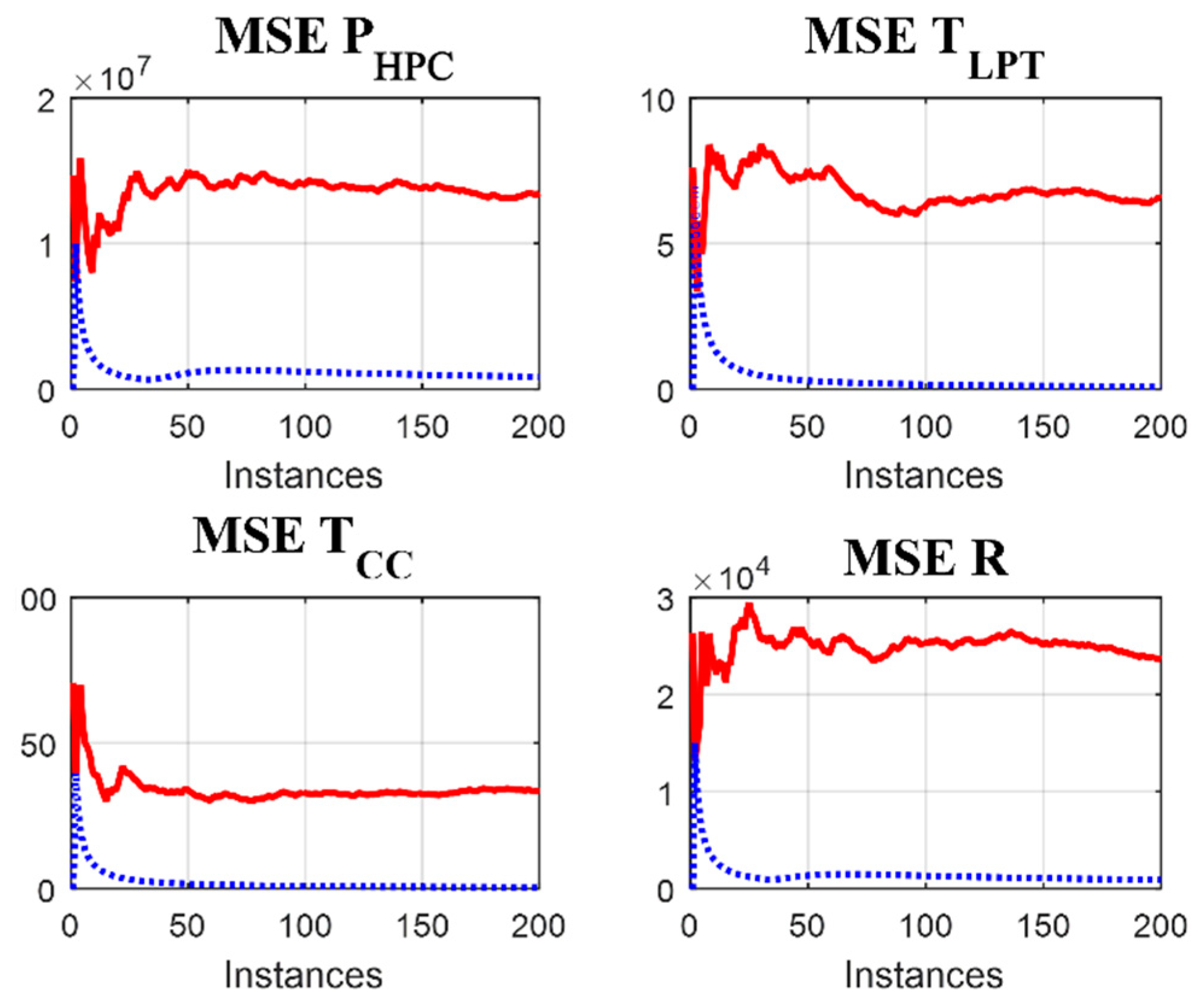
To quantify the filtering effect, two variations of the mean square error (MSE) were computed for each variable: one between the initial noisy values and the exact values and the second between the filtered values and the exact values.
Figure 8 shows these two variations of the MSE against time instances for the same four variables
,
TLPT,
TCC, and
R analyzed before. Comparing the MSE of the initial and filtered values of each variable, we can confirm that the errors after the filtration decrease rapidly and are by far smaller than the initial errors.
In real on-board implementation, the significant noise suppression effect illustrated above will result in more precise variables in control algorithms and, in general, more accurate engine control. The use of the Kalman filter in an on-board diagnostic subsystem will provide more precise estimates of the fault parameters, and, consequently, more reliable engine diagnosis.
6. Real-Time Response Analysis
A real-time system (RTS) implemented in a digital computer interacts with the physical world through the conditioning variables (sensors, actuators, and two converters: Analog/Digital and Digital/Analog) and processes them by a task in real-time,
. As shown in [
3], a real-time task
is described as an executable job entity characterized by arrival and restriction times associated with an instance
, where
i is the task index, and
k is the instance index, see [
4]. The real-time task has many internal tasks, each one with its execution time
limited by a maximum deadline
. These temporal variables can be defined as follows:
Execution time is the time in which the instance with k index of a real-time task carries out its operations.
Deadline is the maximum time in which a local response from the RTS must be obtained, without modification of the dynamic process.
As shown in [
3], real-time systems can be classified as critical and non-critical according to the time limits, synchrony, and quality of response of the environment that interacts with the RTS. For critical RTS, every instance must satisfy
; for non-critical RTS. the condition
is sufficient. For a RTS that is programmed on a digital computer and operates in parallel with a physical system, the analysis of execution times and the fulfillment of the time restrictions (
) justify that this RTS works in real-time.
In our case, the gas turbine measurement filtering is performed with the frequency of 20 Hz that corresponds to the interval 5–20 Hz of engine controllers [
9]. The noise of real engine sensors is also considered. Given the frequency chosen, a 10 s time period is presented by 200 instances with an interval of 50 ms, and the deadline for all instances is
. This time resolution is higher than the resolution observed in the figures of simulated dynamic processes in published studies [
22,
23,
24,
25].
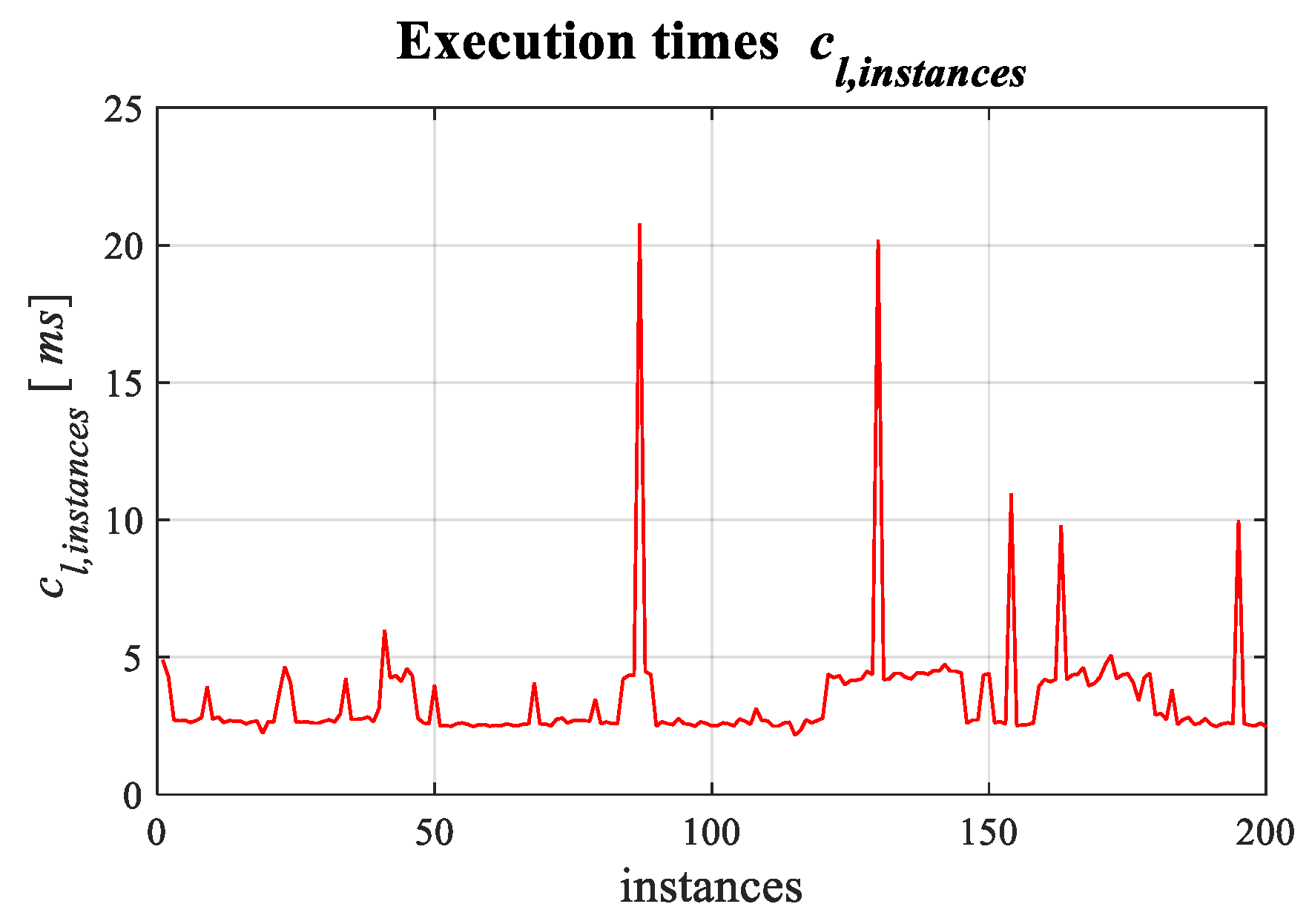
Figure 9 shows the results of this real-time simulation in the form of the execution time plotted for each instance. It can be denoted that the execution time is by far smaller than the deadline; this confirms that all instances achieve the requirements of the real-time operation for a critical real time system. A total execution time of the hybrid dynamic model with the Kalman filter is about 0.8 s. In contrast, the nonlinear dynamic model with no filtering runs 15 s the same transient and, therefore, cannot be used for real-time simulation.
7. Conclusions
In this paper, a turbofan engine for a passenger airplane was analyzed. Since the turbofan presents a complex and expensive mechanical system, to avoid real engine operation, the measurements were previously generated by the hybrid dynamic model and a Kalman filter was integrated to filter measurement errors. The RTS was programmed and operates on the SBC.
The development and validation of this new technique for filtering gas turbine measurements in real-time were performed. To verify the possibility of real-time operation, the algorithm was implemented on the SBC Raspberry Pi 2® with the Emlid RT real-time operating system. First, the chosen gas turbine engine was simulated by the hybrid dynamic model and its accuracy was validated. Then, based on the MSE analysis, the operation of the filtering algorithm was verified; it was found that the algorithm performs the filtering correctly and suppresses measurement noise. Finally, execution time in every time instance was determined, and it was shown that the proposed filtering algorithm has the capacity to work in real-time, which is a strong requirement for its use in real gas turbine control and diagnosis systems.

 ,
, 


