Abstract
The ever-increasing complexity of industrial and engineering problems poses nowadays a number of optimization problems characterized by thousands, if not millions, of variables. For instance, very large-scale problems can be found in chemical and material engineering, networked systems, logistics and scheduling. Recently, Deb and Myburgh proposed an evolutionary algorithm capable of handling a scheduling optimization problem with a staggering number of variables: one billion. However, one important limitation of this algorithm is its memory consumption, which is in the order of 120 GB. Here, we follow up on this research by applying to the same problem a GPU-enabled “compact” Genetic Algorithm, i.e., an Estimation of Distribution Algorithm that instead of using an actual population of candidate solutions only requires and adapts a probabilistic model of their distribution in the search space. We also introduce a smart initialization technique and custom operators to guide the search towards feasible solutions. Leveraging the compact optimization concept, we show how such an algorithm can optimize efficiently very large-scale problems with millions of variables, with limited memory and processing power. To complete our analysis, we report the results of the algorithm on very large-scale instances of the OneMax problem.
1. Introduction
In recent years, several application domains have shown a constantly growing need for efficient optimization algorithms capable of handling problems with a very large number of decision variables, i.e., problems in the order of thousands, or even millions, of variables. Nowadays, this kind of problems occurs for instance in network optimization, logistics, and scheduling: examples of such problems are resource allocation, vehicle routing, and production scheduling, to name a few.
Of note, most of these industrial problems can be formulated in terms of (Mixed) Integer Linear Programming (MILP), and as such can be solved by popular commercial or open-source solvers such as CPLEX [1], Gurobi [2], or glpk [3]. While these solvers are guaranteed to find the optimal solutions, when it comes to solve problems with a very large number of variables, they hit a roadblock. As reported in [4], even on some Linear Programming problems, these solvers are not able to find a feasible solution in feasible time: the so-called “curse of dimensionality”.
A valid alternative to overcome this issue is represented by meta-heuristics, namely stochastic search algorithms which trade optimality guarantees off for better scalability and numerical complexity. Among these, Evolutionary Algorithms (EAs) and Swarm Intelligence—such as Particle Swarm Optimization (PSO)—have especially attracted a great research attention, due to their flexibility and attributed general-purposedness. This is demonstrated by a rich literature in the field, not to mention the various benchmarks and competitions dedicated to Large-Scale Global Optimization (LSGO) [5]. However, perhaps also because these benchmarks focus on continuous optimization, most of the attempts in this area are limited to the continuous domain, with few exceptions. The most notable of these is represented by a recent work by Deb and Myburgh [4,6], who reported to have broken for the first time the “billion-variable barrier” on an ILP problem concerning metallurgy casting scheduling. This achievement was obtained with a Genetic Algorithm dubbed PILP (Population-Based Integer Linear Programming), consisting of two populations (parent and offspring) of 60 solutions each. As the authors reported, the flip side of this method is its memory consumption, which with one billion variables is in the order of 120 GB of RAM: despite the low-cost availability of RAM to date, this is a fairly large amount of memory resources.
This leads us to the motivation of our work. The main research question we try to answer here is: Is it possible to reach at least comparable results to those reported by Deb and Myburgh, with less memory?. Secondly, we try to assess if there is a trade-off between memory consumption and time to solve the problems. As working case, we consider a scenario where one needs to solve very large-scale problems with the additional constraint to save as much as possible the available RAM, while trying to use only one GPU. This memory-constraint scenario further exacerbates the difficulty of solving very large-scale problems, and as such our research question is quite challenging.
A possible answer to our question comes from a concept known as “compact optimization” [7]. Compact optimization is a way of designing stochastic search algorithms belonging to the class of Estimation of Distribution Algorithms (EDAs) [8]. As EDAs, compact optimization algorithms are essentially meta-heuristics that make use of an explicit probabilistic model of the distribution of the solutions in the search space. During the search, new candidate solutions are sampled from the distribution and evaluated; then the model is updated depending on the feedback from the search process itself, such that the next sampling process will be biased towards the most promising areas of the search space. The distinctive feature of compact optimization algorithms [7] with respect to the more general class of EDAs is that they purposely employ a simplistic probabilistic model that handles each variable separately. This model is usually referred to as “Probability Vector” (PV), and its structure and cardinality depend on the problem dimensionality (n) and variable type (binary, integer, or continuous). For instance, in binary problems, the PV simply consists of an n-dimensional vector of probabilities (i.e., each ith element of PV, , represents the probability in that the corresponding ith variable is sampled as 0). In continuous optimization, compact algorithms usually employ n independent truncated Gaussian Probability Distribution Functions (one per variable), and as such the PV consists of two n-dimensional vectors, and , namely means and standard deviations, one per each truncated Gaussian PDF. In this case, sampling involves calculating the inverse of the corresponding Cumulative Distribution Function (see [7] for details).
In the past decade, the compact optimization paradigm has steadfastly advanced. Originally devised mainly as a tool for binary optimization [9,10], many compact algorithms intelligence have been proposed lately, although most of them are meant for continuous optimization only. These include real-valued compact Genetic Algorithm (cGA) [11] (and the similar “Selfish Gene” Algorithm [12]), compact Differential Evolution (cDE) [13,14] and its many variants [15,16,17,18,19,20,21], compact Particle Swarm Optimization (cPSO) [22], compact Bacterial Foraging Optimization (cBFO) [23], and, more recently, compact Teaching Learning Optimization (cTLBO) [24], compact Flower Pollination Algorithm (cFPA) [25], compact Firefly Algorithm (cFA) [26], and compact Artificial Bee Colony (cABC) [27,28]. In terms of applications, these algorithms have been successfully applied to a broad range of memory-limited cases, such as embedded control of robots [29,30,31,32], intrinsic evolvable hardware [33], neural network training [34], and topology control in Wireless Sensor Networks [35].
Obviously, the use of a limited-memory probabilistic model that completely replaces a population comes at a cost. The first drawback concerns the lack of a population, which in turn poses a number of problems in terms of exploration efficiency and loss of diversity: these issues are in fact implicitly addressed by having a sufficiently large number of—possibly diverse—candidate solutions at any given time during the search process, which is the main reason for the success of population-based algorithms [36]. This is by definition impossible in compact algorithms, even though various mechanisms such as re-initialization of the PV or partial restarts [37,38] have been proposed to partially alleviate this problem and prevent premature convergence.
The second drawback comes from the fact that compact algorithms treat all variables as independent. This is not the case of all problems though: most optimization problems are indeed non-separable, i.e., they are characterized by mutual dependencies between variables. These can be captured only by multivariate distributions, similar to the Covariance Matrix used in CMA-ES for continuous optimization [39]. However, due to quadratic space and time complexity, using such distributions in very large-scale problems is not be feasible, unless iterative transformation matrices are used [40]. In discrete optimization, a possible solution is to use approximations of the objective function [41], although the research in this field has been so far rather limited. Notwithstanding these limitations on separability, compact algorithms have proven successfully at solving even non-separable problems, especially at large dimensionalities [7]. One possible explanation for this—somehow surprising—result was given by Caraffini et al. [42], who collected evidence on the fact that the correlation between pairs of variables appears, from the perspective of a stochastic search algorithm, to consistently decrease when the problem dimensionality increases. In other words, non-separable problems in high dimensionalities can be tackled as if they are separable. In [42], the authors conjectured that this effect is due to fact that in high dimensionalities only a very restricted portion of the decision space can be explored: because of this “localness” of the search, the best strategy to make use of the available budget is to exploit any improvement along each variable, which is in accordance with the most popular and successful methods for large-scale optimization.
In this paper, we build on this conjecture and question if, in practice, GPU-enabled cGAs are a viable solution for solving even very large-scale optimization problems. In particular, we focus on the casting scheduling ILP problem tackled by Deb and Myburgh in [4,6] and evaluate the efficacy of a GPU-enabled compact Genetic Algorithm on it. To complete our analysis, we also assess the performance of the cGA on the OneMax benchmark problem [43], both on the original binary formulation, as well as a continuous and an integer formulation with 16 discrete values (reported in Appendix A), on which we evaluate the time consumption of each element of the algorithm. It is worth noting that, apart from [4,6], only few works have tried to apply Evolutionary Algorithms to very large-scale problems: in [44], a one-billion variable noisy binary OneMax problem is tackled with a parallel implementation of cGA on a cluster of 256 CPU cores, with a very weak “relaxed convergence” criterion requiring each variable to reach a fixed-proportion correct value (probability ). In [45], random embeddings are used as a form of dimensionality reduction applied to Bayesian optimization, and tested on a two-variable real-parameter problem embedded into a one-billion variable vector (in which all but two variables have no effect on the fitness). As for a GPU-enabled cGA, thus far the only attempt was made by Iturriaga and Nesmachnow [46], who tested the algorithm on the binary OneMax problem, with and without noise. However, even though their experiments were scaled up to one billion variables, they did not consider the presence of constraints, nor they tackled ILP problems. Therefore, here we advance with respect to the previous literature by: (1) extending the analysis on the OneMax performed in [46], also in the light of the new hardware available (more specifically, Iturriaga and Nesmachnow [46] used 8 CPU cores (Intel Xeon @ 2.33 GHz with 8 GB RAM) in multi-threading, with 4 Tesla C1060 GPUs (each with 4GB GDDR3, 240 cores @ 610 MHz). Here, we use one CPU core (Intel i9-7940x @ 3.10 GHz with 64 GB RAM), with one Titan XP GPU (with 12 GB GDDR5X, 3840 cores @ 1405 Mhz)); and (2) applying, for the first time, a cGA to the very large-scale industrial ILP problem taken from [4,6]. Overall, the main contributions of this work can be summarized as follows:
- We adapt the binary compact Genetic Algorithm in order to handle integer variables, represented in binary form.
- We present a fully GPU-enabled implementation of the compact Genetic Algorithm, where all the algorithmic operations (sampling, model update, solution evaluation, and comparison) can be optionally executed on the GPU.
- We apply the proposed GPU-enabled compact Genetic Algorithm to the OneMax benchmark problem and the casting scheduling ILP problem described in [4,6], in various dimensionalities.
- For the ILP problem, we include in the compact Genetic Algorithm custom (problem-specific) operators and a smart initialization technique inspired by Deb and Myburgh [4] that, by acting on the PV, guide the sampling process towards feasible solutions.
- We show that on the OneMax problem our proposed GPU-enabled compact Genetic algorithm obtains partial improvements with respect to the results reported in [46]; on the casting scheduling problem, we obtain at least comparable–and in some cases better—results with respect to those in [4,6], despite a much more limited usage of computational resources.
The remaining of this paper is organized as follows. In the next section, we describe the formulation of the OneMax and the casting scheduling problems. In Section 3, we introduce the details of the proposed GPU-enabled compact Genetic Algorithm and its various versions. Then, in Section 4, we present the numerical results on the two problems. Finally, in Section 5, we provide the conclusions and highlight possible future research directions.
2. Problem Formulations
Let us introduce the two problems we use in our experimentation. It should be noted that both problems are scalable, i.e., they can be instantiated in any number of variables. In our experiments, we scaled both problems at various dimensionalities, up to one billion variables.
2.1. OneMax
The first problem we used in our experiments is the binary OneMax benchmark function, also called BitCounting [43]. This problem consists in finding a Boolean vector such that:
where is the ith element of , , and . The optimum of this function corresponds to a vector whose all bits are set to one, .
In our experiments, we further extended the original binary formulation of the OneMax problem to account for discrete values () and for continuous variables (). In the first case, the optimum is a vector where all variables are set to 15, and its fitness is . In the second case, the optimum is the same as in the original binary OneMax formulation. We report these additional results in Appendix A.
2.2. Casting Scheduling Problem
The second problem we consider is the casting scheduling ILP problem defined in [4,6], formulated as follows:
where each variable is in . The goal is to find the optimal scheduling to cast batches of N distinct objects in H heats. The production of each ith heat is bound by the corresponding crucible size . Each jth object has a weight, , and must be produced in a certain number of copies, . However, the total amount of metal required for one batch of copies of the same object does not necessarily result equal to the size of the crucible in the ith heat, . For this reason, a desired efficiency is set. This is done by finding the minimum number of heats, H, such that , where M is the total amount of metal required for all batches, . Note that the problem must consider both the fact that the metal molten in one heat cannot be greater than the crucible capacity and that an exact number of objects is required. Therefore, the problem has variables, H inequality constraints, see Equation (3), and N equality constraints, see Equation (4).
To allow the cGA to handle the constraints, we follow the penalty-based approach described in [4,6], by subtracting to the fitness function described in Equation (2) the following quadratic penalty factor, calculated from the constraint violations:
where indicates that the penalty is summed only if the corresponding inequality constraint is violated. Consequently, the cGA should be applied to maximize , where R is a penalty multiplier. However, as suggested in [4,6] and further verified by us, optimal solutions in terms of fitness can be obtained simply by minimizing the penalty factor, i.e., . Note that, while the range of F(x) is , the function takes values in . For this reason, we minimize Equation (5) until it reaches the value 0, which corresponds to in Equation (2).
3. Proposed Algorithms
To better highlight the changes required to the original cGA [9] to make it run on a GPU and handle integer values, we present here separately two versions of the GPU-enabled cGA, namely a binary cGA and a discrete cGA, the latter being an evolution of the first. Their general structure is similar, and is shown in Algorithm 1. Note that the only parameter of both algorithms is virtualPopulation, which affects the dynamics of the algorithm [7]. In a nutshell, the differences between the two algorithms are: (1) the different type of variables (binary vs integer); and (2) the introduction of problem-specific operators in the discrete cGA. Furthermore, for the binary cGA, we present three different versions, i.e., synchronous and asynchronous with sub-problem size 1 and 100 (where “sub-problem” indicates a set of variables handled by one GPU thread). In the following, we describe the details of the GPU implementation of each function used in Algorithm 1 for the various versions of the cGA.
| Algorithm 1 Binary cGA: general structure. |
|
3.1. Binary cGA
We developed in total three versions of the binary cGA, which we refer to as “cGA-Base”, “cGA-A100”, and “cGA-A1”, respectively. Each version follows the structure of Algorithm 1. A summary of the variables and functions used in these binary cGAs is reported in Table 1. The differences among the three versions are in the parallelization process, in particular in the evaluate() and updatePV() functions. cGA-Base operates synchronously, evaluating solutions atomically and, as result, performing updatePV() considering all variables. The two other versions are based on the asynchronous cGA presented in [46], in which the problem is divided into sub-problems of the same size, which are processed asynchronously. In cGA-A100 and cGA-A1, we consider sub-problems sizes of 100 and 1, respectively. Overall, the three versions of the binary cGA differ not only in terms of performance (as we show in the next section), but also in terms of the resources used, which are summarized in Table 2. Let us now analyze in detail the implementation of the three binary cGA versions. For each function used in the cGAs, we specify if it is specific for the OneMax problem or not. If another problem were to be solved, those functions would need to be changed.

Table 1.
Variables and functions used in the binary cGAs.

Table 2.
Data type and size for the binary cGAs.
3.1.1. Binary cGA-Base
In this version of the binary cGA, the parallelization occurs at variable level, i.e., each ith variable is handled by a separate GPU thread. The functions in Table 1 are implemented as follows.
- -
- generateTrial(): This function samples, for each variable, a random number in , and compares it to the corresponding element of PV. If the random number is greater than the element of PV, then the relative variable of trial is set to 1; otherwise, it is set to 0. Each variable is handled by a separate GPU thread.
- -
- compete(): This function compares fitnessTrial and fitnessElite, and sets winner to 1 (0) if trial is better (worse) than elite. This operation is performed without GPU-parallelization.
- -
- evaluate(): This function loops through all the variables of the argument and sums 1 if the ith variable is set to 1. This operation is performed without GPU-parallelization, since its output (the fitness of the argument) depends on all variables.Note: This function is specific for the OneMax problem.
- -
- updatePV(): This function biases PV towards the winner between trial and elite, i.e., it makes more probable that the next trial will be more similar to the winner, increasing or decreasing each element of PV accordingly (see Algorithm 2). Each variable is handled by a separate GPU thread.
| Algorithm 2 Binary cGA-Base: updatePV(). |
|
3.1.2. Binary cGA-A100
In contrast with the cGA-Base, in this case, there is not a one-to-one relation between variables and GPU threads. Instead, each GPU thread handles a single sub-problem, in this case of 100 variables, in particular in the evaluate(), compete() and updatePV() functions. On the contrary, generateTrial() is implemented as in the cGA-Base (i.e., with parallelization at variable level). Furthermore, as it is necessary to save the partial fitness and winner for each sub-problem, in this case fitnessTrial, fitnessElite, and winner are vectors of size problemSize/100 (as shown in Table 2), to allow asynchronous updates. The evaluate(), compete(), and updatePV() functions are implemented as follows.
- -
- evaluate(): This function evaluates the argument by processing each sub-problem independently on the GPU threads. Each thread takes a portion of the argument and calculates its partial fitness. The operations executed by each thread, illustrated in the outer for loop in Algorithm 3, can be parallelized since each sub-problem operates over disjoint portions of the argument. The function getSubProblem() returns the ith sub-problem, i.e., a vector of 100 variables. Note that in this case evaluate() returns a vector, fitness, rather than a scalar. The partial result of each sub-problem is stored by each GPU thread in the corresponding position of fitness.Note: This function is specific for the OneMax problem.
- -
- compete(): This function operates over the vectors fitnessTrial and fitnessElite returned by the evaluate() shown in Algorithm 3. As shown in Algorithm 4, each separate GPU thread simply checks the winner on its sub-problem, i.e., it operates on a single index of fitnessTrial, fitnessElite, and winner, which are all vector of size problemSize/100.Note: This function is specific for the OneMax problem.
- -
- updatePV(): This function is implemented similarly to the evaluate(). As shown in Algorithm 5, each GPU thread loads its portion of data, composed by both corresponding sub-problem of elite and trial and the relative portion of winner and PV. After that, the procedure is similar to the one described in the cGA-Base (see Algorithm 2), with the only difference being that in this case the for loop in Algorithm 2 is performed within the same GPU thread and not in parallel. The ancillary function setPartialPV() updates PV with the result of the partial pPV.Note: This function is specific for the OneMax problem.
| Algorithm 3 Binary cGA-A100: evaluate(). |
|
| Algorithm 4 Binary cGA-A100: compete(). |
|
| Algorithm 5 Binary cGA-A100: updatePV(). |
|
3.1.3. Binary cGA-A1
In principle, this version can be obtained simply by setting the sub-problem size equal to 1 in cGA-A100. However, in this way, the size of winner, fitnessTrial, and fitnessElite would match the problem size, thus increasing the memory usage. For this reason, we decided to embed the operations of evaluate() and compete() into the updatePV() function, thus removing the need for the winner vector and reducing the fitnessTrial and fitnessElite vectors to a scalar. As for the parallelization process, in this case, each GPU thread handles a single variable, as it happens in the cGA-Base. The generateTrial() function is implemented as in the cGA-Base. The updatePV() function is implemented as follows, and replaces Lines 7–13 in Algorithm 1.
- -
- updatePV(): This function includes, in this case, also the operations performed in evaluate() and compete() and results quite simpler than the previous cases. The process is shown in Algorithm 6. Since PV is updated only when the variables of trial and elite are different, each GPU thread checks if one of the two variables is set to 1 and the other to 0. Consequently, PV is only reduced, which increases the probability of sampling 1. Finally, if the relative element of trial is set to 1, each GPU thread adds 1 to the fitnessTrial variable to calculate the total fitness. Note that in this case there is no need for using winner, which reduces the memory consumption.Note: This function is specific for the OneMax problem.
| Algorithm 6 Binary cGA-A1: updatePV(). |
|
3.2. Discrete cGA
The discrete version of the cGA can be seen as an evolution of the binary cGA, specifically adapted to handle integers and include problem-specific mechanisms to solve the casting scheduling problem taken from [4,6]. As for the integer handling, the idea is to represent, quite straightforwardly, integer variables in binary format, and then use a binary cGA to evolve the resulting bit-string. For the casting scheduling problem, we consider integer variables in the interval , and represent each variable with 4 bits. In addition to that, we implement on the GPU the problem-specific smart initialization, crossover and mutation operators described in [4]. We further improve the initialization mechanism in order to adapt it to the cGA paradigm. A summary of the variables and functions used in the discrete cGA is reported in Table 3. The overall structure of the algorithm is shown in Algorithm 7. In the following, we describe the main implementation details of the discrete cGA. Note that, unless indicated differently, all operations are fully parallelized on the GPU, maintaining a one-to-one mapping between GPU threads and variables as described in the cGA-Base.
| Algorithm 7 Discrete cGA: specific structure for the cast scheduling problem. |
|

Table 3.
Variables and functions used in the discrete cGA.
- -
- smartInitialization(): This function performs the initialization process, divided into three steps. Firstly, the function estimateH() estimates the value H to get an efficiency equal to , as described in Section 2.2. This value is also used to define the size of elite and PV. Secondly, an elite of size is created in initializeElite(), repaired by the two mutations, and evaluated. Finally, PV is created, with a size of and processed as described in initializePV() below.
- o
- initializeElite(): This function initializes the elite as described in [4], i.e., creates the elite by creating N vectors of size H, which are initialized respecting as much as possible the number of copies required for each object. This operation is GPU-parallelized through two steps: firstly, a vector of random numbers is created, and a correction factor is calculated; and, secondly, the correction is applied to the vector. After this, to repair any possible violated constraint, the elite is passed to the two mutation operators mutationOne() and mutationTwo(), and finally evaluated by evaluate(). The implementation of these functions is shown below.
- o
- initializePV(): This function initializes the PV such that it generates solutions that satisfy the inequality constraints, and which are biased towards the elite. This initialization is performed in two functions. The first function, shown in Algorithm 8, blocks the PV values for the variables which, if set to 1, would cause the violation of an inequality constraint. For example, if the crucible size is 600 kg and an object weights 200 kg, obviously no more than three copies can be cast for that object without a penalty: in this case, the inhibitor blocks (i.e., sets to NaN) the third and fourth bit of the variable, preventing it from assuming values greater than 3 for that object. This operation is GPU-parallelized, with each thread checking a single element of PV. The second function aims at modifying the PV values to produce solutions closer to the elite. This operation is done by setting each PV element to if the bit of the corresponding element in the elite is 1, and otherwise, unless that element is blocked by inhibitor(), as shown in Algorithm 9.
- -
- generateTrial(): This function is divided into four steps: generation of the trial, crossover and two mutation operators to repair the trial. The problem-specific crossover and mutation operators were implemented as described in [6]. In addition, we operated some modifications in order to parallelize the operators on the GPU and save the information necessary to simplify the successive calculation of the fitness. This information consists of two vectors, one of size H, called heatsTrial, and one of size N called copiesTrial. The first one saves the available space in the crucible for each heat, and it is created during newTrial() in two steps: firstly, the vector is initialized with the crucible size; then, while trial is created, its values are decreased, as shown in Algorithm 10. Moreover, heatsTrial is updated also during crossover and mutations, as shown below. The second vector, copiesTrial, stores instead the total number of objects cast by the trial, and is calculated during mutationOne() (see Algorithm 12). The other details of the four steps are presented below.
- o
- newTrial(): This function, as shown in Algorithm 10, is implemented such that each GPU thread handles one variable of trial and its corresponding four values of PV. More specifically, each thread samples 4 bits based on the corresponding probabilities of PV, converts them to a value in , and assigns this value to the corresponding variable in trial. Finally, the element of heatsTrial relative to this variable is updated accordingly to the value just assigned. Note that this last operation is implemented as thread-safe, as the same heat can be updated asynchronously by different threads.
- o
- crossover(): The function, as shown in Algorithm 11, is implemented such that each GPU thread handles one variable of trial. The crossover operator compares each heat of trial with the corresponding one in elite. If elite has a better heat (i.e., has a higher (lower) value in case both trial and elite have negative (positive) heats), then all the elite variables referred to that heat are assigned to trial, updating heatsTrial accordingly.
- o
- mutationOne(): The first mutation is meant to repair trial with respect to the equality constraint (see Equation (4)). The procedure is divided into two steps, as shown in Algorithm 12: firstly, the total number of copies cast by trial for each object, copiesTrial, is calculated, with each GPU thread handling one variable of trial and performing a thread-safe sum over copiesTrial. Next, for each object, if the copies required (stored in copies) are less than the ones that are cast (stored in copiesTrial), this means that some copies in excess should be removed from trial: to do that, first the heat with the greatest inequality violation (i.e., the lowest value of heatsTrial, returned by argmin()) is found, then the corresponding variable in trial is decreased by one, and heatsTrial and copiesTrial are updated accordingly. On the other hand, if the copies required are more than the ones that are cast, this means that some more copies should be added to trial: to do that, first the heat with the lowest crucible utilization (i.e., the highest value of available space, stored in heatsTrial, returned by argmax()) is found, then the corresponding variable in trial is increased by one, and heatsTrial and copiesTrial are updated accordingly. This operation is repeated until the equality constraint is satisfied. Note that the functions used to find the two heats, i.e., argmin() and argmax(), are GPU-parallelized. Moreover, during the repair process heatsTrial and copiesTrial vectors are updated in order to be reused later to calculate the fitness.
- o
- mutationTwo(): The second mutation tries to reduce the heats which use more space than the one available in the crucible, as described in [4]. The procedure consists in finding two heats: the one with the greatest inequality violation, and the one with the greatest available space. After that, a random object is selected and removed from the first heat and added to the second one, in order to preserve the total number of copies. These operations are repeated the number of times indicated by the parameter iterationLimit. In the original version in [4], this value was fixed during all the computation (set to 30), while, in our implementation, due to the compact nature of the algorithm, we needed to double this value at each iteration, starting from 30. This process leads to an exponential increase of the time of mutationTwo(), as shown in the next section. As for the parallelization process, similar to mutationOne(), it is obtained by loading trial into the GPU and then performing the argmin() and argmax() operations parallelized with a one-to-one mapping between GPU threads and variables.
- -
- evaluate(): This function evaluates the solution in a time-efficient way, using the information already calculated during generateTrial(). The two penalty factors related to the inequality and equality constraints (see Equations (3) and (4)) are determined, respectively, through the heatsTrial and copiesTrial vectors, and added to fitnessTrial, as shown in Algorithm 13. The total time required is , and it is further decreased due to the parallelization over H heats. Note that the second loop over N objects is not parallelized as N is typically much smaller than H.
- -
- updatePV(): This function is parallelized on the size of PV (one bit per GPU thread) and operates similarly to Algorithm 2, with the only difference that each thread has to extract the relative bit before performing the update.
| Algorithm 8 Discrete cGA: inhibitor(). |
|
| Algorithm 9 Discrete cGA: initializePV(). |
|
| Algorithm 10 Discrete cGA: newTrial(). |
|
| Algorithm 11 Discrete cGA: crossover(). |
|
| Algorithm 12 Discrete cGA: mutationOne(). |
|
| Algorithm 13 Discrete cGA: evaluate(). |
|
4. Results
We discuss now the performance of the binary and discrete cGA implementations described in the previous section. Firstly, we compare the three binary cGAs (cGA-Base, cGA-A100, and cGA-A1) with the cGA presented in [46] on the OneMax problem. Then, we compare the discrete cGA with the PILP algorithm presented in [4,6]. We provide the code publicly as Colab notebooks (https://drive.google.com/drive/folders/1k6KWtR9ceuW7HneLptK3TlMpfjqaNMBT?usp=sharing).
4.1. OneMax
We performed the experiments on the OneMax problem using the Google®Colab service, which provides a machine powered by an Intel®Xeon™4 CPU @ 2.20 GHz, 25 GB RAM, with an NVIDIA®P100 GPU. For each algorithm presented, we tested four dimensionalities, varying the size of the problem from one million to one billion variables. For each algorithm and problem size, we performed 10 runs, with a virtual population of 100. Each run ended either when it reached the optimal fitness, or after a predetermined maximum number of iterations (note that in the cGA one iteration corresponds to one solution evaluation). This last parameter was set to 5000 for all the dimensionalities, except for the case with one billion variables, where it was set to 1600 for the cGA-Base and cGA-A100 and 500 for the cGA-A1. A summary of the results, in comparison with the results taken from [46], is shown in Table 4 for the synchronous cGAs, and in Table 5 for the asynchronous cGAs.

Table 4.
Synchronous binary cGAs: comparison on the OneMax problem (mean across 10 runs, std. dev. in parentheses). The symbol ‘-’ indicates data not provided in [46].

Table 5.
Asynchronous binary cGAs: comparison on the OneMax problem (mean across 10 runs, std. dev. in parentheses). The symbol ’-’ indicates data not provided in [46].
Our cGA-Base shows only marginal improvements with respect to the cGA-sync from [46]. One possible explanation for this is the different value of virtual population used in [46], which however is not reported in the paper. However, as it is quite improbable that a compact genetic algorithm can converge in very large-scale problems [44], our result can be considered satisfactory. In contrast with these results, our asynchronous versions show much better results, in terms of both computing time and fitness. In particular, the cGA-A100 obtains better results in all four dimensionalities, with execution times from 9 to 46 times smaller than the times reported in [46] (also due to more recent GPU hardware). The cGA-A1, as expected, shows even better behavior, solving the problem in roughly 1300 iterations for the first three dimensionalities, and reaching in only 500 iterations for the one billion-variable problem. The fitness trend of the three binary cGAs is shown in Figure 1, where it can be seen that, while the synchronous cGA suffers from premature convergence, the asynchronous cGAs do not, and are able to reach high-quality solutions in both versions of the algorithm, although with a very different convergence profile: the cGA-A100 shows an almost-linear behavior, while the cGA-A1 has an exponential convergence.

Figure 1.
Best fitness value per iteration (mean ± std. dev. across 10 runs per algorithm) for the three binary cGAs on the OneMax problem in four different dimensionalities.
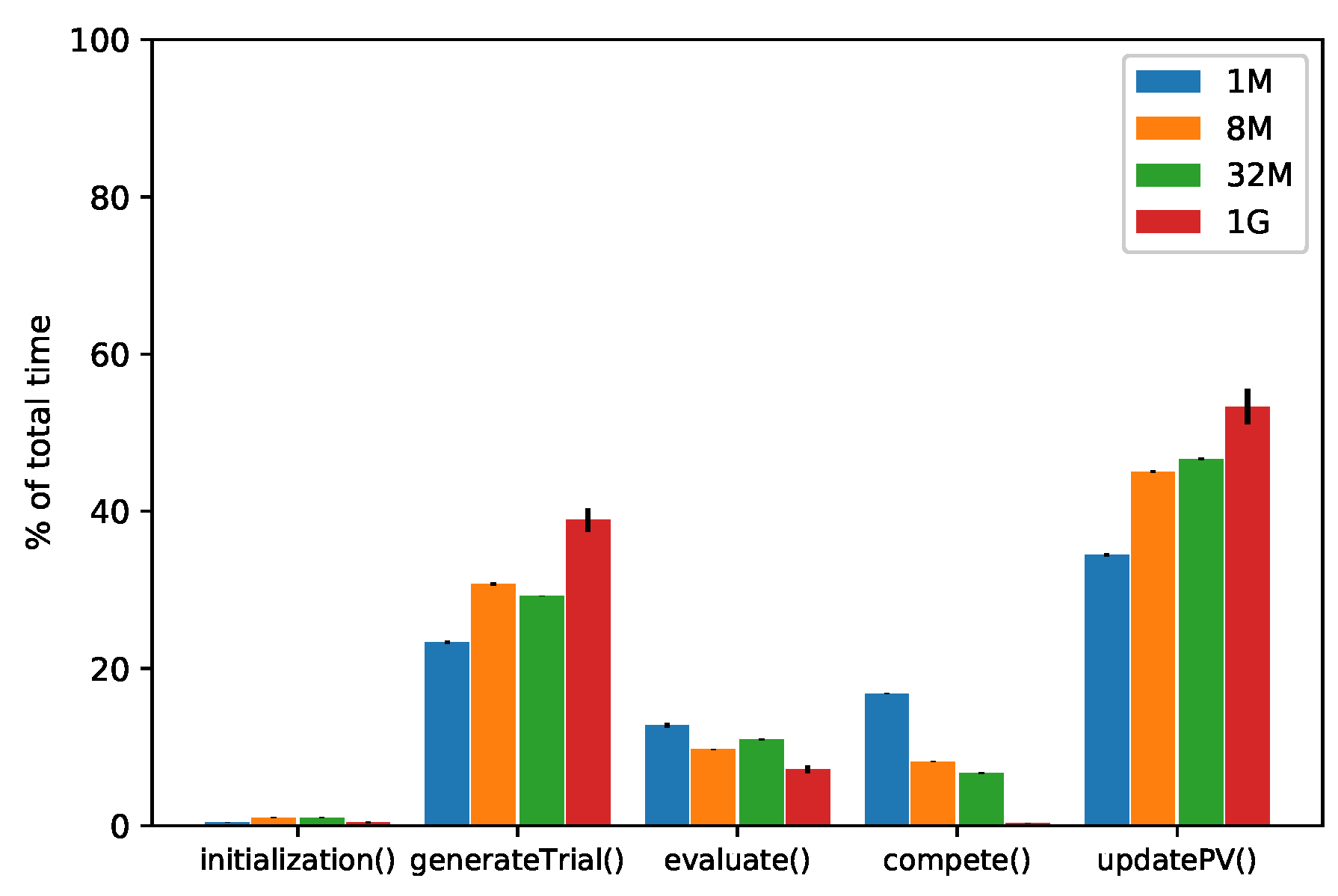
We complete our analysis on the OneMax problem with a profiling of the various functions used in the cGAs. The results for the cGA-A100 are shown in Figure 2, where it can be noted that the time distribution on the four problem dimensionalities is approximately the same, with the updatePV() and generateTrial() functions requiring most of the time, roughly and , respectively. The remaining is divided between evaluate() and compete(). Similar considerations apply to the cGA-Base and cGA-A1, with some caveats: Firstly, as described in the previous section, the compete() function in the asynchronous algorithms is more expensive than in the cGA-Base. Secondly, in the cGA-A1 the operations of compete() and evaluate() are embedded into updatePV(), causing an increase of this function in terms of execution time. Interestingly, these results are quite different from the ones described in [46], where up to of the time is spent in the trial generation phase, while in our setup most of the time is spent to update the probability vector.

Figure 2.
Time profiling (mean ± std. dev. across 10 runs) for the cGA-A100 on the OneMax problem in four different dimensionalities.
4.2. Casting Scheduling Problem
We performed the experiments on the casting scheduling problem on a Linux workstation powered by an Intel®Core™i9-7940x CPU @ 3.10GHz, 64GB RAM, with an NVIDIA®Titan XP GPU. The code was tested on Ubuntu 19.10 (kernel GNU/Linux 5.3.0-40-generic x86_64), CUDA 10.1, and Python3 with the Numba library used to write the GPU kernel for the parallelization process.
Similar to the OneMax case, we ran 10 independent runs of the discrete cGA for three different dimensionalities (100k, 1M, and 10M variables), with and the input parameters indicated in Table 6. The virtualPopulation and the iterationLimit are set to 100 and 30, respectively. Of note, all the runs terminated successfully, finding the optimal solution corresponding to . A summary of the results in comparison with the results taken from [4] is shown in Table 7.

Table 6.
Parameters used for the casting scheduling problem. Note that the crucible size, W, and the weights are in common for all the problem dimensionalities, therefore the only parameter that changes across dimensionalities is the number of copies per object.

Table 7.
Casting scheduling problem: number of solution evaluations to reach the optimum, number of heat updates, and execution times (mean across 10 runs, std. dev. in parentheses). The results for the PILP algorithm are taken from Table 6 in [4]; the symbol ‘-’ indicates data not provided.
It should be noted that our implementation requires only a few tens of solution evaluations to solve the problem (slightly more than 50 in the 10M case), while PILP for the same problem dimensionalities needs above 1000 evaluations. This reflects also in an average number of heat updates (i.e., how many times a variable is modified by the two mutation operators), which is from 10 to 300 times lower than PILP, due to the lower number of trials processed. Additionally, it is important to consider the much smaller amount of memory used with respect to the population-based PILP algorithm: while discrete cGA needs only bytes (More specifically: float32 (for PV), int8 (for trial and elite), and int32 (for ).) to save PV, trial, elite and its respective heats vector, PILP requires bytes, where 60 is the population size, excluding some additional memory needed to store the fitness values and other data structures.
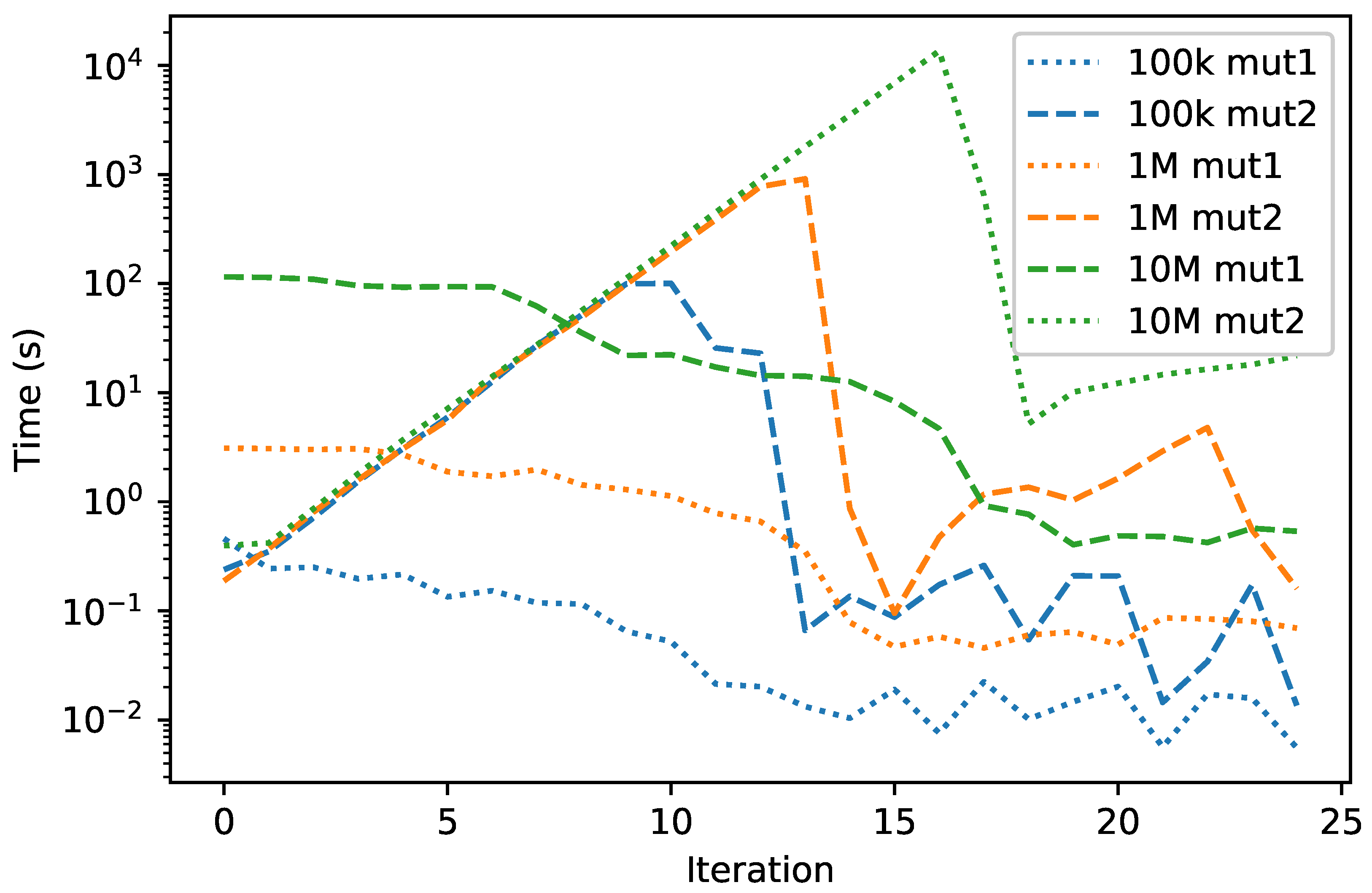
As for the time needed to solve the problem, our algorithm results from one to two orders of magnitude slower than PILP. This is mainly due to the lack of a population, which we compensated with an exponential increase of the parameter iterationLimit in mutationTwo(). As can be seen in Table 7, the majority of time is spent for the generateTrial() function, particularly for the execution of the mutation operators. As shown in Figure 3, during the first iterations, the execution times for the two mutations is dominated by mutationOne(), but eventually it is mutationTwo() that requires more time. However, it can be seen that the time per iteration of mutationTwo() remains almost constant as the problem dimensionality increases. Therefore, the time increase of mutationTwo() is only caused by the increasing number of iterations required. Overall, it seems then that there is a trade-off between memory consumption (more memory is needed to store more solutions, which allow a better search with fewer iterations needed to repair them) and time to converge (with limited memory, more time is needed to repair the trial generated at each iteration of the cGA).
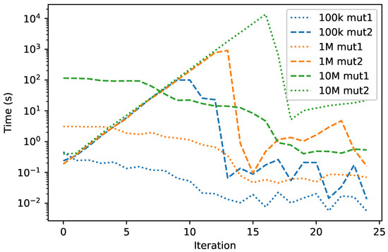
Figure 3.
Execution time per iteration (mean across 10 runs) for the two mutation operators on the casting scheduling problem in three different dimensionalities.
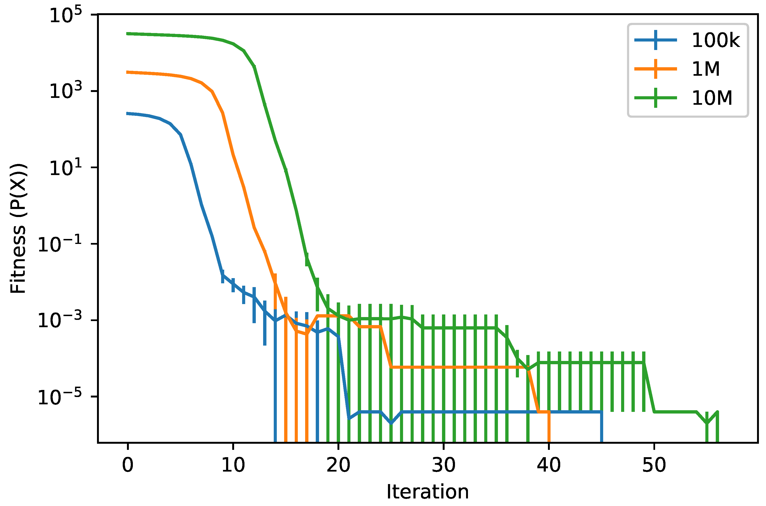
For completeness, we report the fitness trend of the discrete cGA in Figure 4. The behavior is similar to the one described in [4], with the entire evolution that can be divided into three phases: in the initial galloping phase, the fitness rapidly decreases; then follows a consolidation phase, where new solutions have small improvements; and, lastly, the final solution is created in the culmination phase.
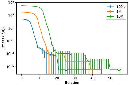
Figure 4.
Best fitness value per iteration (mean ± std. dev. across 10 runs) on the casting scheduling problem in three different dimensionalities.
Effect of the Smart PV Initialization
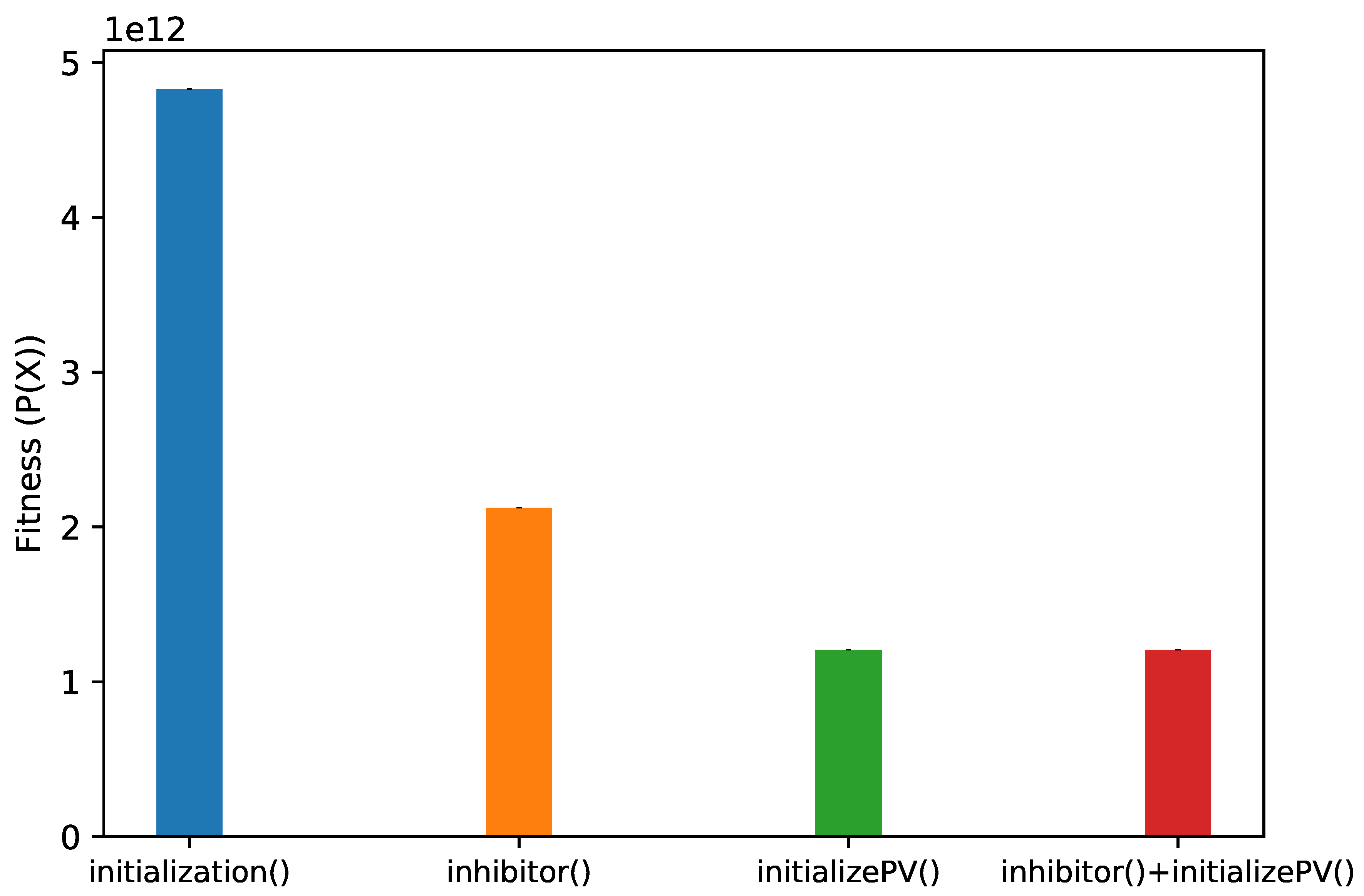
As discussed in the previous section, for the casting scheduling problem, we introduced a smart initialization mechanism aimed at reducing the fitness of the first trial and also avoiding generating unfeasible solutions. To assess the effect of the smart initialization on the algorithmic performance, we compared the effect of inhibitor() and initializePV() with that of a random initialization. As shown in Figure 5, these two functions lead to generate trials that are five times better (in terms of fitness) than those generated by random initialization, indicated as initialization(). This provides the algorithm a “head start” that as seen before allows converging in a very limited number of iterations.
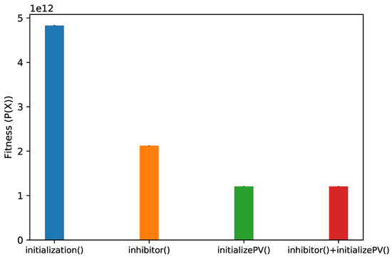
Figure 5.
Casting scheduling problem: fitness of trials generated using different PV initialization strategies (mean ± std. dev. across 1000 trials). Here, initialization() indicates a random initialization of PV. Note that in these experiments the mutation operators are not applied, thus any violated constraint is not repaired. While it seems that initializePV() alone is enough to generate good trials at the beginning of the algorithm, inhibitor() blocks the bits also during the evolution.
5. Conclusions
In many application domains, there is a constant demand for ever more efficient optimization techniques. This is especially true for large-scale optimization problems, for which one usually needs large computational resources—in terms of processing power and memory—to obtain a reasonable solution in feasible time. However, in some cases, the available computational resources might be scarce, or should be reserved to other applications. Therefore, it is of great interest to find a trade-off between efficient optimization and resource consumption.
In this study, we tackled very large-scale optimization problems (of up to one billion variables), in both discrete and continuous domains, with special constraints on processing power and memory. In particular, we questioned if it is possible to solve these kinds of problems by fitting efficiently the search algorithm into one GPU. To do that, we considered a compact Genetic Algorithm (cGA) and we adapted it to make it work on the GPU, by splitting the problem and letting multiple GPU cores work in parallel on different sub-problems. We considered two different sub-problem sizes (1 and 100). In addition, we implemented both asynchronous and synchronous schemes, depending on the possibility of updating the best solution as soon as an improvement is found on one sub-problem.
To test the proposed algorithm, we considered binary, integer, and continuous optimization problems. In particular, we first benchmarked the algorithm on the OneMax problem in binary, integer (16 values) and continuous settings. Then, we considered an industrial casting scheduling problem recently presented by Deb and Myburgh [6]. Overall, our numerical results show that: (1) compact optimization techniques are a viable solution for solving very large-scale problems even with limited resources; and (2) they are especially suitable for GPU-parallelization. On the other hand, compact algorithms have some implicit limitations deriving from the fact that they lack a population of candidate solutions, hence being in general less efficient at exploring the search space compared to population-based algorithms. Therefore, to use these algorithms properly in practical applications—without sacrificing too much the optimization performances—it is recommended to couple them with problem knowledge. To show this, here we demonstrated how a base version of the cGA can be customized, for the specific case of the scheduling problem, with a smart initialization of the probability vector (that is, the probabilistic model used in the compact algorithm) aimed at guiding the search towards feasible solutions, as well as problem-specific mutation and crossover operators aimed at repairing constraint violations, adapted from [6]. Furthermore, we adapted the cGA to handle variables of different kinds, as well as equality and inequality constraints.
In future works, we aim to further extend cGAs by hybridizing them with other single-solution optimization algorithms, such as simulated annealing [47], and applying gradient-based methods to perform local search, in a memetic fashion. Furthermore, we will consider the use of decomposition techniques (either problem-aware or problem-agnostic) and restart mechanisms such as the re-sampled inheritance introduced in [37,38]. Another intriguing possibility would be to integrate compact algorithms with a quantum annealer, to obtain a hybrid quantum-classical optimizer. Finally, it will be interesting to apply these algorithms to other domains, e.g. for training deep neural networks, in Wireless Sensor Networks applications [48], or to solve very large-scale instances of TSP and other “NK landscape” problems, as recently discussed in [49,50].
Author Contributions
Conceptualization, G.I.; Data curation, A.F.; Formal analysis, A.F.; Investigation, A.F.; Methodology, G.I.; Software, A.F.; Supervision, G.I.; Validation, A.F.; Visualization, A.F.; Writing—original draft, A.F. and G.I.; Writing—review & editing, G.I. Both authors contributed equally to this work. Both authors have read and agreed to the published version of the manuscript. All authors have read and agreed to the published version of the manuscript.
Funding
This research received no external funding.
Acknowledgments
We gratefully acknowledge the support of NVIDIA Corporation with the donation of the TITAN Xp GPU used for this research.
Conflicts of Interest
The authors declare no conflict of interest.
Appendix A. Additional Results on OneMax Problem
Appendix A.1. Discrete OneMax
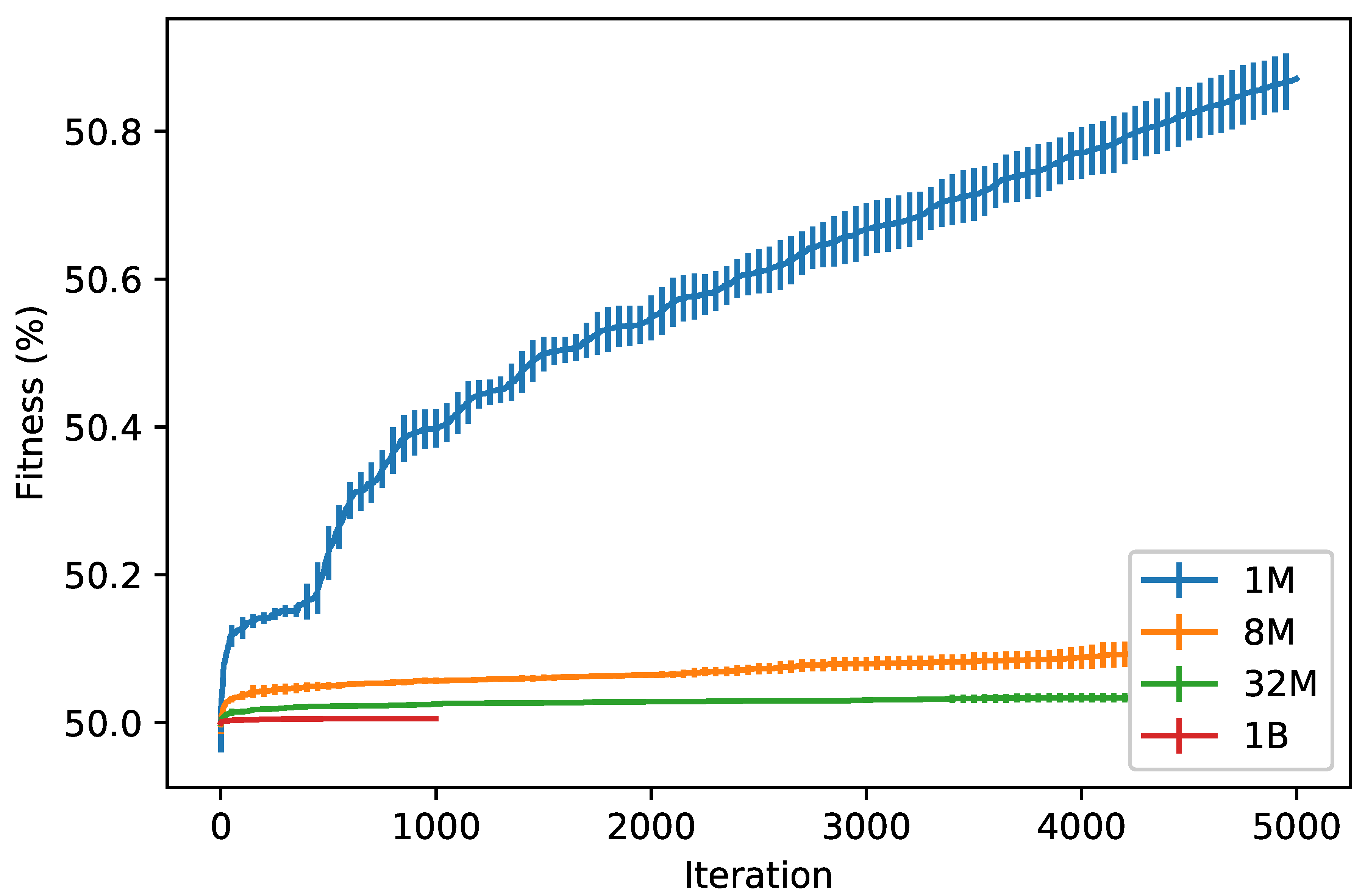
We present here additional results obtained with the discrete cGA on a discrete version of the OneMax problem. For this analysis, we used the general version of the discrete cGA presented in Section 3.2, where we removed all the problem-dependent operations implemented for the casting scheduling problem, namely the smartInitialization(), crossover(), mutationOne() and mutationTwo() functions. The algorithm obtained has a structure similar to Algorithm 1, but it is able to handle integers variables. Similar to the casting scheduling problem, we considered integer variables in the interval .
- -
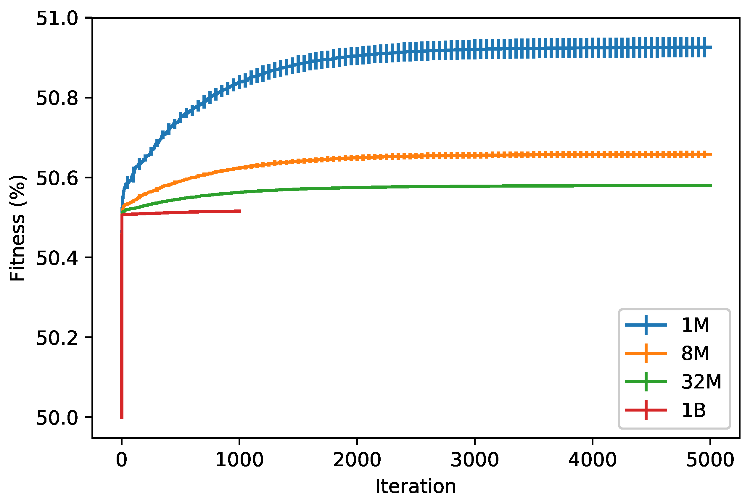
- Results: We performed 10 runs on four dimensionalities, setting the virtualPopulation to 100. The maximum number of iterations was set to 5000 for problem instances up to 32M variables and 1000 for the 1B case. All experiments were executed on the Google®Colab service. The results obtained, reported in Table A1, are similar to the results reported in Section 4.1 for the binary OneMax problem, although times are (up to) twice as big. The main reason for this time increase is the fact that in this case the algorithm handles 4 bits per variable in the newTrial() and updatePV() functions, instead of just one as in the binary cGA.

Table A1.
Results of the cGA on the discrete and continuous OneMax problem.
Table A1.
Results of the cGA on the discrete and continuous OneMax problem.
| Discrete cGA | Continuous cGA | |||||||
|---|---|---|---|---|---|---|---|---|
| 1M | 8M | 32M | 1B | 1M | 8M | 32M | 1B | |
| Time (s) | 72.463 (2.038) | 395.806 (3.985) | 1958.932 (485.963) | 13,143.343 (3201.053) | 156.647 (1.487) | 985.936 (118.716) | 3366.755 (20.297) | 20,895.186 (4131.433) |
| Fitness (%) | 50.926 (0.0250) | 50.658 (0.008) | 50.579 (0.002) | 50.515 (0.0005) | 50.870 (0.039) | 50.102 (0.024) | 50.034 (0.0072) | 50.0055 (0.0003) |
| Iterations | 5000 | 5000 | 5000 | 1000 | 5000 | 5000 | 5000 | 1000 |
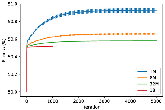
Figure A1.
Best fitness value per iteration (mean ± std. dev. across 10 runs per algorithm) for the cGA on the discrete OneMax problem in four different dimensionalities.
Figure A1.
Best fitness value per iteration (mean ± std. dev. across 10 runs per algorithm) for the cGA on the discrete OneMax problem in four different dimensionalities.
Appendix A.2. Continuous OneMax
We also implemented a GPU-enabled continuous cGA, based on the original algorithm proposed in [11], with some modifications. As a benchmark, we considered the OneMax problem where all variables can take real values in , instead of binary values. The main difference with respect to the binary and discrete cGAs is the sampling procedure and the update of PV. As briefly mentioned in Section 1, the continuous cGA uses for each variable a truncated Gaussian PDF, and to sample new value it calculates the inverse of the corresponding CDF. Therefore, the probability vector in this case consists of 2 vectors which describe the mean and standard deviation of the Gaussian PDFs (see [7] for details). As for the parallelization process, we implemented a scheme similar to the binary cGA-Base, using a one-to-one mapping between variables and GPU threads, both for the operations in common with the cGA-Base and for the functions described below.
- -
- Algorithm: The main modifications we added to the original cGA scheme illustrated in Algorithm 1 include mutation and crossover operators, inspired by Differential Evolution (DE) [13], and an adaptive restart mechanism. All these mechanisms are problem-independent.
- o
- Mutation: The value of each variable is obtained by sampling three values from the relative Gaussian PDF, and then combining them as in the rand/1 DE [13]:where F is a parameter, and sample() is the procedure to sample from the Gaussian PDF.
- o
- Crossover: We implemented two different strategies, based on the binomial and exponential crossover used in DE. Both are based on a parameter , but their behavior is different. In the binomial crossover, each variable in a trial copies with probability the corresponding variable from the elite. In the exponential crossover, starting from a random position, the variables of the trial are copied from the elite, until a random number is greater than .
- o
- Restart: The adaptive restart mechanism partially restarts the evolution by resetting the values trough two parameters. The first parameter, invariant, controls when to apply the restart, which can occur for two reasons: either if for invariant consecutive iterations the trial does not improve the elite, or if the trial improves it but the improvement (i.e., the difference between its fitness and that of the elite) is less than . The second parameter regulates the portion of variables involved, i.e., each variable as a probability to be reset. Finally, the new value of after each restart changes dynamically during the evolution process: in particular, it starts from 10, it is doubled every time a restart occurs and it is halved every time there are invariant iterations without a restart.
- -
- Results: We tested separately the different behavior of the two crossover strategies, the impact of three different algorithm configurations (base, i.e., without DE-mutation and crossover; with mutation and crossover; and with mutation, crossover and restart), and how the algorithm scales. For this analysis, we used the parameters shown in Table A2. All the experiments were executed on the Google®Colab service.
- o
- Crossover strategies: We tested the two crossover strategies over 5000 iterations on the continuous OneMax problem with 1M variables. As shown in Figure A2, the two crossover strategies show a similar behavior, although the exponential crossover tends to reach a plateau earlier than the binomial crossover.
- o
- Algorithm configurations: In this case as well, the different configurations were tested over 5000 iterations on the continuous OneMax problem with 1M variables, using the binomial crossover. As shown in Figure A3, the restart greatly enhances the algorithm’s performance, avoiding premature convergence and also increasing the fitness achieved. It is important to consider that the parameters involved in the restart procedure must be chosen carefully in order to avoid making the search ineffective.
- o
- Scalability: As shown in Figure A4, the results are similar, in terms of behavior, to the binary and discrete cases, shown earlier in Figure 1 and Figure A1. However, the final fitness values are slightly worse. This is mainly due to two reasons: firstly, the continuous domain leads to smaller fitness increases; and, secondly, the chosen restart parameters seem to work well in the 1M case, but not on larger dimensionalities. It is also of note that the total execution time results from two to four times bigger than the equivalent binary and discrete cases.

Table A2.
Parameter settings for the cGA applied to the continuous OneMax problem.
Table A2.
Parameter settings for the cGA applied to the continuous OneMax problem.
| Parameter | Value |
|---|---|
| virtualPopulation | 100 |
| F | |
| (binomial) | |
| (exponential) | |
| invariant | 300 |
| resetPR |
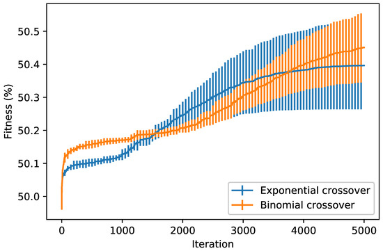
Figure A2.
Best fitness value per iteration (mean ± std. dev. across 10 runs) for the cGA with two different crossover operators on the continuous OneMax problem in 1M dimensions.
Figure A2.
Best fitness value per iteration (mean ± std. dev. across 10 runs) for the cGA with two different crossover operators on the continuous OneMax problem in 1M dimensions.

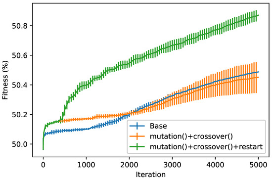
Figure A3.
Best fitness value (mean ± std. dev. across 10 runs) for the cGA with different configurations on the continuous OneMax problem in 1M dimensions.
Figure A3.
Best fitness value (mean ± std. dev. across 10 runs) for the cGA with different configurations on the continuous OneMax problem in 1M dimensions.

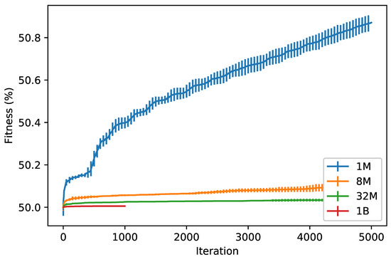
Figure A4.
Best fitness value per iteration (mean ± std. dev. across 10 runs per algorithm) for the cGA on the continuous OneMax problem in four different dimensionalities.
Figure A4.
Best fitness value per iteration (mean ± std. dev. across 10 runs per algorithm) for the cGA on the continuous OneMax problem in four different dimensionalities.
References
- CPLEX IBM ILOG, User’s Manual for CPLEX. Available online: https://www.ibm.com/support/knowledgecenter/SSSA5P_12.7.1/ilog.odms.cplex.help/CPLEX/homepages/usrmancplex.html (accessed on 1 April 2020).
- Gurobi Optimization Inc. Gurobi Optimizer Reference Manual. Available online: https://www.gurobi.com/wp-content/plugins/hd_documentations/documentation/9.0/refman.pdf (accessed on 1 April 2020).
- Makhorin, A. GLPK (GNU Linear Programming Kit). Available online: https://www.gnu.org/software/glpk/ (accessed on 1 April 2020).
- Deb, K.; Myburgh, C. A population-based fast algorithm for a billion-dimensional resource allocation problem with integer variables. Eur. J. Oper. Res. 2017, 261, 460–474. [Google Scholar] [CrossRef]
- Omidvar, M.N.; Li, X. Evolutionary large-scale global optimization: An introduction. In Proceedings of the Genetic and Evolutionary Computation Conference Companion, Berlin, Germany, 15–19 July 2017; pp. 807–827. [Google Scholar]
- Deb, K.; Myburgh, C. Breaking the billion-variable barrier in real-world optimization using a customized evolutionary algorithm. In Proceedings of the Genetic and Evolutionary Computation Conference, Denver, CO, USA, 20–24 July 2016; pp. 653–660. [Google Scholar]
- Neri, F.; Iacca, G.; Mininno, E. Compact Optimization. In Handbook of Optimization: From Classical to Modern Approach; Springer: New York, NY, USA, 2013; pp. 337–364. [Google Scholar]
- Lozano, J.A.; Larra naga, P.; Inza, I.; Bengoetxea, E. Towards a New Evolutionary Computation: Advances on Estimation of Distribution Algorithms; Springer: New York, NY, USA, 2006; Volume 192. [Google Scholar]
- Harik, G.R.; Lobo, F.G.; Goldberg, D.E. The compact genetic algorithm. IEEE Trans. Evol. Comput. 1999, 3, 287–297. [Google Scholar] [CrossRef]
- Ahn, C.W.; Ramakrishna, R.S. Elitism-based compact genetic algorithms. IEEE Trans. Evol. Comput. 2003, 7, 367–385. [Google Scholar]
- Mininno, E.; Cupertino, F.; Naso, D. Real-Valued Compact Genetic Algorithms for Embedded Microcontroller Optimization. IEEE Trans. Evol. Comput. 2008, 12, 203–219. [Google Scholar] [CrossRef]
- Corno, F.; Reorda, M.S.; Squillero, G. The Selfish Gene Algorithm: A New Evolutionary Optimization Strategy. In ACM Symposium on Applied Computing; ACM: New York, NY, USA, 1998; pp. 349–355. [Google Scholar]
- Mininno, E.; Neri, F.; Cupertino, F.; Naso, D. Compact differential evolution. IEEE Trans. Evol. Comput. 2011, 15, 32–54. [Google Scholar] [CrossRef]
- Iacca, G.; Caraffini, F.; Neri, F. Compact Differential Evolution Light: High Performance Despite Limited Memory Requirement and Modest Computational Overhead. J. Comput. Sci. Technol. 2012, 27, 1056–1076. [Google Scholar] [CrossRef]
- Mallipeddi, R.; Iacca, G.; Suganthan, P.N.; Neri, F.; Mininno, E. Ensemble strategies in Compact Differential Evolution. In Proceedings of the Congress on Evolutionary Computation, New Orleans, LA, USA, 5–8 June 2011; pp. 1972–1977. [Google Scholar]
- Iacca, G.; Mallipeddi, R.; Mininno, E.; Neri, F.; Suganthan, P.N. Super-fit and population size reduction in compact Differential Evolution. In Proceedings of the Workshop on Memetic Computing, Paris, France, 11–15 April 2011; pp. 1–8. [Google Scholar]
- Iacca, G.; Mallipeddi, R.; Mininno, E.; Neri, F.; Suganthan, P.N. Global supervision for compact Differential Evolution. In Proceedings of the Symposium on Differential Evolution, Paris, France, 11–15 April 2011; pp. 1–8. [Google Scholar]
- Iacca, G.; Neri, F.; Mininno, E. Opposition-Based Learning in Compact Differential Evolution. In Proceedings of the Conference on the Applications of Evolutionary Computation, Dublin, Ireland, 27–29 April 2011; pp. 264–273. [Google Scholar]
- Iacca, G.; Mininno, E.; Neri, F. Composed compact differential evolution. Evol. Intell. 2011, 4, 17–29. [Google Scholar] [CrossRef]
- Neri, F.; Iacca, G.; Mininno, E. Disturbed Exploitation compact Differential Evolution for limited memory optimization problems. Inf. Sci. 2011, 181, 2469–2487. [Google Scholar] [CrossRef]
- Iacca, G.; Neri, F.; Mininno, E. Noise analysis compact differential evolution. Int. J. Syst. Sci. 2012, 43, 1248–1267. [Google Scholar] [CrossRef]
- Neri, F.; Mininno, E.; Iacca, G. Compact Particle Swarm Optimization. Inf. Sci. 2013, 239, 96–121. [Google Scholar] [CrossRef]
- Iacca, G.; Neri, F.; Mininno, E. Compact Bacterial Foraging Optimization. In Swarm and Evolutionary Computation; Springer: Berlin/Heidelberg, Germany, 2012; pp. 84–92. [Google Scholar]
- Yang, Z.; Li, K.; Guo, Y. A new compact teaching-learning-based optimization method. In International Conference on Intelligent Computing; Springer: Cham, Switzerland, 2014; pp. 717–726. [Google Scholar]
- Dao, T.K.; Pan, T.S.; Nguyen, T.T.; Chu, S.C.; Pan, J.S. A Compact Flower Pollination Algorithm Optimization. In Proceedings of the International Conference on Computing Measurement Control and Sensor Network, Matsue, Japan, 20–22 May 2016; pp. 76–79. [Google Scholar]
- Tighzert, L.; Fonlupt, C.; Mendil, B. A set of new compact firefly algorithms. Swarm Evol. Comput. 2018, 40, 92–115. [Google Scholar] [CrossRef]
- Dao, T.K.; Chu, S.C.; Shieh, C.S.; Horng, M.F. Compact artificial bee colony. In Proceedings of the International Conference on Industrial, Engineering and Other Applications of Applied Intelligent Systems, Kaohsiung, Taiwan, 3–6 June 2014; pp. 96–105. [Google Scholar]
- Banitalebi, A.; Aziz, M.I.A.; Bahar, A.; Aziz, Z.A. Enhanced compact artificial bee colony. Inf. Sci. 2015, 298, 491–511. [Google Scholar] [CrossRef]
- Jewajinda, Y. Covariance matrix compact differential evolution for embedded intelligence. In Proceedings of the IEEE Region 10 Symposium, Bali, Indonesia, 9–11 May 2016; pp. 349–354. [Google Scholar]
- Neri, F.; Mininno, E. Memetic compact differential evolution for Cartesian robot control. IEEE Comput. Intell. Mag. 2010, 5, 54–65. [Google Scholar] [CrossRef]
- Iacca, G.; Caraffini, F.; Neri, F. Memory-saving memetic computing for path-following mobile robots. Appl. Soft Comput. 2013, 13, 2003–2016. [Google Scholar] [CrossRef]
- Iacca, G.; Caraffini, F.; Neri, F.; Mininno, E. Robot Base Disturbance Optimization with Compact Differential Evolution Light. In Conference on the Applications of Evolutionary Computation; Springer: Berlin/Heidelberg, Germany, 2012; pp. 285–294. [Google Scholar]
- Gallagher, J.C.; Vigraham, S.; Kramer, G. A family of compact genetic algorithms for intrinsic evolvable hardware. IEEE Trans. Evol. Comput. 2004, 8, 111–126. [Google Scholar] [CrossRef]
- Yang, Z.; Li, K.; Guo, Y.; Ma, H.; Zheng, M. Compact real-valued teaching-learning based optimization with the applications to neural network training. Knowl. -Based Syst. 2018, 159, 51–62. [Google Scholar] [CrossRef]
- Dao, T.K.; Pan, T.S.; Nguyen, T.T.; Chu, S.C. A compact artificial bee colony optimization for topology control scheme in wireless sensor networks. J. Inf. Hiding Multimed. Signal Process. 2015, 6, 297–310. [Google Scholar]
- Prugel-Bennett, A. Benefits of a Population: Five Mechanisms That Advantage Population-Based Algorithms. IEEE Trans. Evol. Comput. 2010, 14, 500–517. [Google Scholar] [CrossRef]
- Caraffini, F.; Neri, F.; Passow, B.N.; Iacca, G. Re-sampled inheritance search: High performance despite the simplicity. Soft Comput. 2013, 17, 2235–2256. [Google Scholar] [CrossRef]
- Iacca, G.; Caraffini, F. Compact Optimization Algorithms with Re-Sampled Inheritance. In Conference on the Applications of Evolutionary Computation; Springer: Cham, Switzerland, 2019; pp. 523–534. [Google Scholar]
- Hansen, N.; Müller, S.D.; Koumoutsakos, P. Reducing the time complexity of the derandomized evolution strategy with covariance matrix adaptation (CMA-ES). Evol. Comput. 2003, 11, 1–18. [Google Scholar] [CrossRef]
- Loshchilov, I.; Glasmachers, T.; Beyer, H.G. Large scale black-box optimization by limited-memory matrix adaptation. IEEE Trans. Evol. Computat. 2018, 23, 353–358. [Google Scholar] [CrossRef]
- Halman, N.; Kellerer, H.; Strusevich, V.A. Approximation schemes for non-separable non-linear boolean programming problems under nested knapsack constraints. Eur. J. Oper. Res. 2018, 270, 435–447. [Google Scholar] [CrossRef]
- Caraffini, F.; Neri, F.; Iacca, G. Large scale problems in practice: the effect of dimensionality on the interaction among variables. In Conference on the Applications of Evolutionary Computation; Springer: Cham, Switzerland, 2017; pp. 636–652. [Google Scholar]
- Schaffer, J.; Eshelman, L. On crossover as an evolutionarily viable strategy. In Proceedings of the International Conference on Genetic Algorithms, San Diego, CA, USA, 13–16 July 1991; pp. 61–68. [Google Scholar]
- Goldberg, D.E.; Sastry, K.; Llorà, X. Toward routine billion-variable optimization using genetic algorithms. Complexity 2007, 12, 27–29. [Google Scholar] [CrossRef]
- Wang, Z.; Hutter, F.; Zoghi, M.; Matheson, D.; de Feitas, N. Bayesian optimization in a billion dimensions via random embeddings. J. Artif. Intell. Res. 2016, 55, 361–387. [Google Scholar] [CrossRef]
- Iturriaga, S.; Nesmachnow, S. Solving very large optimization problems (up to one billion variables) with a parallel evolutionary algorithm in CPU and GPU. In Proceedings of the IEEE International Conference on P2P, Parallel, Grid, Cloud and Internet Computing, Victoria, BC, Canada, 12–14 November 2012; pp. 267–272. [Google Scholar]
- Xinchao, Z. Simulated annealing algorithm with adaptive neighborhood. Appl. Soft Comput. 2011, 11, 1827–1836. [Google Scholar] [CrossRef]
- Iacca, G. Distributed optimization in wireless sensor networks: an island-model framework. Soft Comput. 2013, 17, 2257–2277. [Google Scholar] [CrossRef]
- Whitley, D. Next generation genetic algorithms: A user’s guide and tutorial. In Handb. Metaheuristics; Springer: Cham, Switzerland, 2019; pp. 245–274. [Google Scholar]
- Varadarajan, S.; Whitley, D. The massively parallel mixing genetic algorithm for the traveling salesman problem. In Proceedings of the Genetic and Evolutionary Computation Conference, Prague, Czech Republic, 13–17 July 2019; pp. 872–879. [Google Scholar]
© 2020 by the authors. Licensee MDPI, Basel, Switzerland. This article is an open access article distributed under the terms and conditions of the Creative Commons Attribution (CC BY) license (http://creativecommons.org/licenses/by/4.0/).


