A Computational Method for Subdivision Depth of Ternary Schemes

Abstract

Subdivision schemes are extensively used in scientific and practical applications to produce continuous shapes in an iterative way. This paper introduces a framework to compute subdivision depths of ternary schemes. We first use subdivision algorithm in terms of convolution to compute the error bounds between two successive polygons produced by refinement procedure of subdivision schemes. Then, a formula for computing bound between the polygon at k-th stage and the limiting polygon is derived. After that, we predict numerically the number of subdivision steps (depths) required for smooth limiting shape based on the demand of user specified error (distance) tolerance. In addition, extensive numerical experiments were carried out to check the numerical outcomes of this new framework. The proposed methods are more efficient than the method proposed by Song et al.

1. Introduction

A broad and eminent area in Computer Aided Geometric Design (CAGD) deals with curves, surfaces, and their computational aspects. Subdivision is the most remarkable field for the purpose of modeling of curves and surfaces in CAGD. Subdivision methods have achieved much popularity in the past few years because of their implementation along with their mathematical formulation. The convolution technique [1] is one of the techniques used to merge different schemes. It has an important role in error analysis of the schemes. Actually, subdivision schemes take the polygons as input and successively produced smooth polygons or shapes as an output. Initially, the schemes with two rules were introduced. Later on, the interest was developed to recommend the schemes with three rules. This means at each subdivision level, every edge of the polygon is divided into three sub-edges. In the literature, these schemes are known as ternary schemes. Here, first we present brief review of these schemes then we will address the problem of error analysis.

Here we present an overview of the ternary subdivision schemes. Mustafa et al. [2,3,4,5] presented a $(2n-1)$-point ternary approximating and interpolating scheme, a 6-point ternary interpolating scheme, a family of even points ternary schemes, the odd point ternary approximating scheme respectively. Hassan et al. [6] and Siddiqi and Rehan [7] threw the light on 4-point ternary interpolating subdivision schemes. Kwan et al. [8] explored the phenomenon of 4-points ternary approximating scheme and Mustafa et al. [9,10] examined 5-point and 6-point ternary interpolating schemes and their differentiability. Siddiqi et al. [11,12] explained 4-point ternary interpolating scheme for curve sketching and constructed different ternary approximating subdivision schemes. Peng et al. [13,14] discovered non-linear circle preserving interpolating scheme and fractal behavior of ternary rational interpolating scheme. Further discussing on ternary subdivision scheme, Aslam [15] and Beccari et al. [16] showed their talent to highlight a family of 5-point non-linear ternary interpolating scheme and an interpolating 4-point ternary non-stationary scheme with tension control respectively. Certainly, there are a few methods for estimating the error bounds of these schemes.

Some of the authors [17,18,19] computed the error and order of the convergence of some binary schemes. Mustafa et al. [20,21,22,23] computed error bounds for binary, ternary, tensor product binary volumetric model and binary non-stationary schemes. Error bounds for a class of subdivision schemes based on the two-scale refinement equation were computed by Moncayo and Amat [24]. A formula for estimating the deviation of a binary interpolating subdivision curve from its data polygon was presented by Deng et al. [25]. However, the generalization of this formula to deal with the cases of n-ary interpolating and approximating schemes is still an open question. The following open question also arises in our mind: “How many subdivision steps (depths) are required to satisfy a user specified error (distance) tolerance?” Some of the researchers can be nominated as the embarking volunteers for the explanation of above questions such as: Mustafa and Hashmi [26] estimated subdivision depth computation for n-ary schemes by using first forward difference technique. Mustafa [27] presented subdivision depth computation technique for tensor product ternary volumetric model. Mustafa et al. also computed subdivision depth for triangular surfaces [28]. The above methods do not work for all type of subdivision schemes. Counter examples are also presented in this paper.

A novel numerical algorithm to estimate the subdivision depth was offered only for binary subdivision schemes in [29]. Still there is a gap/space to work for the subdivision depth of higher arity (i.e., ternary, quaternarys and so on) schemes. In this paper, an optimal approach is proposed to estimate subdivision depths for ternary (i.e., for each subdivision level, every edge of polygon is divided into three sub-edges) subdivision schemes.

The remaining part of the paper is arranged as follows. In Section 2, basic results, subdivision depths and numerical experiments of the method for univariate cases of the schemes are presented while in Section 3, these results for bivariate cases of the schemes are offered. Conclusions are drawn in Section 4.

2. Preliminary Results for Univariate Case

Let $\{p_i^k;i\in \mathbb{Z}\}$ be a sequence of 2D points in ${\mathbf{R}}^{\mathbf{2}}$ which are obtained by the following refinement procedure

$$p_{3i+s}^{k+1}=\sum _{m=0}^{N-1}{a}_{s,m}{p}_{i+m}^k,s=0,1,2,$$

(1)

with

$$\sum _{m=0}^{N-1}{a}_{s,m}=1,s=0,1,2,$$

(2)

where $k\ge 0$ indicates the refinement level. The points at 0th level $p_i^0$ are known as initial control points. The refinement procedure described in (1) along with its necessary condition of converge (2) is known as univariate ternary subdivision scheme. The following formulation of unknown coefficients $a_{s,m}$ is given by [21].

$$\begin{array}{c}\left\{\begin{array}{c}{b}_{0,m}={\displaystyle \sum _{l=0}^m}(a_{0,l}-a_{1,l}),\hfill \\ b_{1,m}={\displaystyle \sum _{l=0}^m}(a_{1,l}-a_{2,l}),\hfill \\ b_{2,m}=a_{0,m}-(b_{0,m}+b_{1,m}),\hfill \end{array}\right.\hfill \end{array}$$

with

$$\sum _{m=0}^{N-1}|b_{0,m}|<1,\sum _{m=0}^{N-1}|b_{1,m}|<1,\sum _{m=0}^{N-1}|b_{2,m}|<1.$$

The following symbolization will also be used in coming section of this paper.

$$\begin{array}{c}\left\{\begin{array}{c}{d}_{3m}=b_{0,m},\hfill \\ d_{3m+1}=b_{1,m},\hfill \\ d_{3m+2}=b_{2,m}.\hfill \end{array}\right.\hfill \end{array}$$

(3)

Now we follow the techniques and notations presented in [24]. To be precise, let the vector $u_i=u_i^k$ represent the approximation coefficients associated with a certain $k^{th}$ level of resolution. If $u_i^0=u_i^{k;0}$ represents the $k^{th}$ resolution level then the reconstruction algorithm used to define the approximation coefficients at stage $k+1$ in terms of the coefficient at stage k are obtained by the use of subdivision algorithms in terms of convolutions i.e.,

$$u_i^{k+1}=\sum _{n\in \mathbb{N}}{d}_{i-3n}{u}_n^k={(u^{k;0}★d)}_i,$$

(4)

where ★ denotes the convolution product of two vectors $u^{k;0}$ and $d={(d_n)}_{n\in \mathbb{N}}$.

Generally, the convolution product of two vectors $u={(u_n)}_{n\ge 0}$ and $v={(v_n)}_{n\ge 0}$ of finite lengths $l_u$ and $l_v$ respectively for ternary subdivision scheme is defined as

$${(u★v)}_j=\sum _{n=max\{j-(l_v-1),0\}}^{min\{j,l_u-1\}}{u}_n{v}_{j-3n},j=0,1,\dots ,l_u+l_v-2.$$

(5)

In the following subsection, we present the generalized version of the results presented in the Appendices A1 and A2 of [24].

2.1. Reformulation of Successive Convolutions

In this subsection, we obtain some generalized inequalities used in order to find the subdivision depth of ternary subdivision schemes for the generation of curves. Their further generalizations are presented in Section 3 for the computation of depth of ternary subdivision schemes for tensor product surfaces. This section contains typical rigorous and tedious mathematical expressions. Readers are refers to Example 1 of this section for better understanding.

Lemma 1.

Let $u=u_n$ be the vector of finite length and $d={\{d_n\}}_{n=0}^{3N-1}$ with $d_n=0$ for $n\ge 3N$, then the following one dimensional $k_0$ convolutions is bounded by

$$\parallel ({(\dots {(({(u^{(0)}★d)}^{(0)})★d)}^{(0)}★\dots ★d)}^{(0)}★d){\parallel }_{\infty }\le {\parallel u\parallel }_{\infty }\underset{j}{sup}\left\{\sum _{m=0}^{\lfloor j/3^{k_0}\rfloor }|B_{m,j}^{k_0}|\right\},$$

where $B_{m,j}^{k_0}$ is defined recursively by

$$\begin{array}{c}\left\{\begin{array}{c}{B}_{m,j}^1=d_{j-3m},\hfill \\ B_{m,j}^{k_0}={\displaystyle \sum _{p=3m}^{\lfloor j/3^{k_0-1}\rfloor }}{B}_{m,p}^1{B}_{p,j}^{k_0-1},k_0\ge 2,\hfill \end{array}\right.\hfill \end{array}$$

and

$$j\in \mathsf{\Sigma }(k_0,N)=\{\mathsf{\Omega }(k_0,N)-3^{k_0}+1,\mathsf{\Omega }(k_0,N)-3^{k_0}+2,\dots ,\mathsf{\Omega }(k_0,N)\},$$

$$\mathsf{\Omega }(k_0,N)=(3^{k_0}-2)(3N-1).$$

Proof. 

To prove this result, we start with the case of $k_0=1$ and $k_0=2$ convolutions and then a general case will be derived.

Case $k_0=1$: From (5), we obtain a relation given in the following

$$|{(u^{(0)}★d)}_j|=|\sum _{n=0}^{\lfloor j/3\rfloor }{u}_n{d}_{j-3n}|,$$

(6)

where $\lfloor .\rfloor$ denotes the integer part. Using infinity norm $\left({\parallel u\parallel }_{\infty }=max\{|u_o|,\dots ,|u_{\lfloor j/3\rfloor }|\}\right)$, we get

$$\begin{array}{ccc}|{(u^{(0)}★d)}_j|\hfill & \le & {\parallel u\parallel }_{\infty }\sum _{n=0}^{\lfloor j/3\rfloor }|d_{j-3n}|.\hfill \end{array}$$

Now

$$\begin{array}{ccc}sup|{(u^{(0)}★d)}_j|\hfill & \le & sup\left({\parallel u\parallel }_{\infty }\sum _{n=0}^{\lfloor j/3\rfloor }|d_{j-3n}|\right).\hfill \end{array}$$

This infers

$$\begin{array}{ccc}sup|{(u^{(0)}★d)}_j|\hfill & \le & {\parallel u\parallel }_{\infty }sup\left(\sum _{n=0}^{\lfloor j/3\rfloor }|B_{n,j}^1|\right),\hfill \end{array}$$

where

$$d_{j-3n}=B_{n,j}^1.$$

(7)

Thus,

$$\parallel {(u^{(0)}★d)}_j{\parallel }_{\infty }\le {\parallel u\parallel }_{\infty }sup\left(\sum _{n=0}^{\lfloor j/3\rfloor }|B_{n,j}^1|\right).$$

Case $k_0=2$: From (6), we acquire

$$\begin{array}{ccc}{({(u^{(0)}★d)}^{(0)}★d)}_j\hfill & =& \sum _{m=0}^{\lfloor j/3\rfloor }{(u^{(0)}★d)}_m{d}_{j-3m}=\sum _{m=0}^{\lfloor j/3\rfloor }\left(\sum _{n=0}^{\lfloor m/3\rfloor }{u}_n{d}_{m-3n}\right)d_{j-3m}.\hfill \end{array}$$

This infers

$$\begin{array}{ccc}{({(u^{(0)}★d)}^{(0)}★d)}_j\hfill & =& u_0{d}_0{d}_j+u_0{d}_1{d}_{j-3}+u_0{d}_2{d}_{j-6}+u_0{d}_3{d}_{j-9}+u_1{d}_0{d}_{j-9}+u_0{d}_4{d}_{j-12}\hfill \\ & +& u_1{d}_1{d}_{j-12}+\dots +u_0{d}_{\lfloor \frac{j}{3}\rfloor }{d}_0+u_1{d}_{\lfloor \frac{j}{3}\rfloor -3}{d}_0+\dots +u_{\lfloor \frac{j}{3^2}\rfloor }{d}_{\lfloor \frac{j}{3}\rfloor -3\lfloor \frac{j}{3^2}\rfloor }{d}_0.\hfill \end{array}$$

This implies that

$$\begin{array}{ccc}{({(u^{(0)}★d)}^{(0)}★d)}_j\hfill & =& \sum _{m=0}^{\lfloor j/3^2\rfloor }{u}_m\left(\sum _{n=3m}^{\lfloor j/3\rfloor }{d}_{n-3m}{d}_{j-3n}\right).\hfill \end{array}$$

This infers

$$\begin{array}{ccc}{({(u^{(0)}★d)}^{(0)}★d)}_j\hfill & =& \sum _{m=0}^{\lfloor j/3^2\rfloor }{u}_m\left(\sum _{n=3m}^{\lfloor j/3\rfloor }{B}_{m,n}^1{B}_{n,j}^1\right)=\sum _{m=0}^{\lfloor j/3^2\rfloor }{u}_m{B}_{m,j}^2,\hfill \end{array}$$

where

$$B_{m,j}^2=\sum _{n=3m}^{\lfloor j/3\rfloor }{B}_{m,n}^1{B}_{n,j}^1.$$

(8)

So

$$|{({(u^{(0)}★d)}^{(0)}★d)}_j|=|\sum _{m=0}^{\lfloor j/3^2\rfloor }{u}_m{B}_{m,j}^2|\le {\parallel u\parallel }_{\infty }\sum _{m=0}^{\lfloor j/3^2\rfloor }|B_{m,j}^2|.$$

This implies

$$\parallel {({(u^{(0)}★d)}^{(0)}★d)}_j{\parallel }_{\infty }\le {\parallel u\parallel }_{\infty }\underset{j}{sup}\left(\sum _{m=0}^{\lfloor j/3^2\rfloor }|B_{m,j}^2|\right).$$

General case: By using the same technique, we acquire the reformulations for $k_0$-th convolutions, which is in the following

$${({(\dots {(({(u^{(0)}★d)}^{(0)})★d)}^{(0)}★\dots ★d)}^{(0)}★d)}_j=\sum _{m=0}^{\lfloor j/3^{k_0}\rfloor }{u}_m{B}_{m,j}^{k_0}.$$

Which implies

$$\parallel ({(\dots {(({(u^{(0)}★d)}^{(0)})★d)}^{(0)}★\dots ★d)}^{(0)}★d){\parallel }_{\infty }\le {\parallel u\parallel }_{\infty }\underset{j}{sup}\left\{\sum _{m=0}^{\lfloor j/3^{k_0}\rfloor }|B_{m,j}^{k_0}|\right\}.$$

(9)

□

Lemma 2.

The term $B_{m,j}^{k_0}$ in the inequality (9) has the following expression

$$B_{m-1,j-3^{k_0}}^{k_0}=B_{m,j}^{k_0}=B_{m+1,j+3^{k_0}}^{k_0}.$$

(10)

Proof. 

Now we start for an induction process, which is over $k_0$. Then

Case $k_0=1$:

$$B_{m,j}^1=d_{j-3m}=d_{j+3-3(m+1)}=B_{m+1,j+3}^1.$$

(11)

Similarly

$$B_{m+1,j}^1=d_{j-3(m+1)}=B_{m,j-3}^1.$$

(12)

From (8), we have

$$B_{m,j}^2=\sum _{n=3m}^{\lfloor j/3\rfloor }{B}_{m,n}^1{B}_{n,j}^1.$$

Using (11), we have

$$B_{m,j}^2=\sum _{n=3m}^{\lfloor j/3\rfloor }{B}_{m,n}^1{B}_{n+1,j+3}^1.$$

(13)

Now replace n by $n-3$ in (13), we obtain

$$B_{m,j}^2=\sum _{n=3(m-1)}^{\lfloor j/3+3\rfloor }{B}_{m,n-3}^1{B}_{n-2,j+3}^1.$$

Now using (12), we acquire

$$B_{m,j}^2=\sum _{n=3(m-1)}^{\lfloor j/3+3\rfloor }{B}_{m+1,n}^1{B}_{n,j+3^2}^1.$$

so

$$B_{m,j}^2=B_{m+1,j+3^2.}^2$$

We suppose that it is true for an integer $k_0=M$, that is

$$B_{m,j}^M=B_{m+1,j+3^M.}^M$$

(14)

Case $k_0=M+1$: Consider

$$B_{m,j}^{M+1}=\sum _{n=3m}^{\lfloor j/3^M\rfloor }{B}_{m,n}^1{B}_{n,j}^M.$$

Using (14), we have

$$B_{m,j}^{M+1}=\sum _{n=3m}^{\lfloor j/3^M\rfloor }{B}_{m,n}^1{B}_{n+1,j+3^M}^M.$$

(15)

Now, replace n by $n-3$ in (15), we have

$$B_{m,j}^{M+1}=\sum _{n=3(m+1)}^{\lfloor j/3^M+3\rfloor }{B}_{m,n-3}^1{B}_{n-2,j+3^M}^M.$$

Using (12) and (14), we acquire

$$\begin{array}{c}{B}_{m,j}^{M+1}=B_{m+1,j+3^{M+1}.}^{M+1}\hfill \end{array}$$

Similarly we can prove

$$\begin{array}{c}{B}_{m,j}^{M+1}=B_{m-1,j-3^{M+1}.}^{M+1}\hfill \end{array}$$

Hence

$$B_{m-1,j-3^{k_0}}^{k_0}=B_{m,j}^{k_0}=B_{m+1,j+3^{k_0}}^{k_0}.$$

□

Now, applying Lemmas 1 and 2, we arrive at the following useful result:

Corollary 1.

The associated constant of a $k_0$-th convolution with vector $d=\{d_0,d_1,\dots ,d_{3N-1}\}$ is

$$D_{k_0}=\underset{j}{sup}\left\{\sum _{m=0}^{\lfloor j/3^{k_0}\rfloor }|B_{m,j}^{k_0}|\right\}=\underset{j\in \mathsf{\Sigma }(k_0,N)}{sup}\left\{\sum _{m=0}^{\lfloor j/3^{k_0}\rfloor }|B_{m,j}^{k_0}|\right\}.$$

(16)

Proof. 

Assume that $d=\{d_0,d_1,\dots ,d_{3N-1}\},$ with $N\in \mathbb{N}$ and $\mathsf{\Omega }(k_0,N)=(3^{k_0}-2)(3N-1).$ Then for $j>\mathsf{\Omega }(k_0,N)$ and by using Lemma 1, we acquire

$$B_{0,j}^{k_0}=0.$$

(17)

Similarly for $j>\mathsf{\Omega }(k_0,N)+m{3}^{k_0}$ and using Lemma 2, we have

$$B_{m,j}^{k_0}=0.$$

(18)

Finally, using (17) and (18), we get (16). □

2.2. Subdivision Depth for Ternary Subdivision Curves

In this section, we first generalize the inequalities (2.18) and then (2.5) which were presented in [21]. After that, we present a numerical inequality to compute the subdivision depth of ternary subdivision schemes for curve modeling.

Theorem 1.

Consider the initial polygon $p_i^0,i\in \mathbb{Z}$ and $p_i^k,k\ge 0$, recursively interpreted by (1) together with (2). Suppose $P^k$ represents the polygon at the points $\{p_i^k\}$. Then after two successive refinements/iterations k and $k+1$, the error bounds between these two iterations is

$$\begin{array}{c}\parallel P^{k+1}-P^k{\parallel }_{\infty }\le \xi \eta {(D_{k_0})}^k,\hfill \end{array}$$

where $D_{k_0},k_0\ge 1$ defined in (16), $\eta =\underset{i}{max}∥p_{i+1}^0-p_i^0∥$ and

$$\begin{array}{ccc}\xi \hfill & =& max\left(\sum _{m=0}^{N-2}\left|{\tilde{a}}_{0,m}\right|,\sum _{m=0}^{N-2}\left|{\tilde{a}}_{1,m}\right|,\sum _{m=0}^{N-2}\left|{\tilde{a}}_{2,m}\right|\right),{\tilde{a}}_{s,m}=\sum _{i=m+1}^{N-1}{a}_{s,i},0\le s\le 2,\hfill \\ {\tilde{a}}_{1,0}\hfill & =& \sum _{i=1}^{N-1}{a}_{1,i}-\frac{1}{3},{\tilde{a}}_{2,0}=\sum _{i=1}^{N-1}{a}_{2,i}-\frac{2}{3}.\hfill \end{array}$$

Proof. 

See in [21]. □

Theorem 2.

Let a limit curve $P^{\infty }$ be linked with the subdivision iterative process, then under the same conditions used in Theorem 1 the following inequality hold

$${∥P^{\infty }-P^k∥}_{\infty }\le \xi \eta \left(\frac{{(D_{k_0})}^k}{1-D_{k_0}}\right),$$

where $k_0\ge 1$ is a natural number, such that $D_{k_0}<1$.

Proof. 

See in [21]. □

Theorem 3.

Let k be subdivision depth and let ${\nabla }^k$ be the error bound between ternary subdivision curve $P^{\infty }$ and its k-level control polygon $P^k$. For arbitrary $ϵ>0$, if

$$k\ge lo{g}_{D_{k_0}}\left(\frac{ϵ(1-D_{k_0})}{\xi \eta }\right),$$

(19)

then ${\nabla }^k\le ϵ$.

Proof. 

Let ${\nabla }^k$ be the distance between limit curve $P^{\infty }$ and control polygon $P^k$ at k-th level defined in Theorem 2, such that

$${\nabla }^k={∥P^{\infty }-P^k∥}_{\infty }\le \xi \eta \left(\frac{{(D_{k_0})}^k}{1-D_{k_0}}\right).$$

To obtain given error tolerance $ϵ>0$, consider

$$\xi \eta \left(\frac{{(D_{k_0})}^k}{1-D_{k_0}}\right)\le ϵ,$$

which implies

$$\frac{\xi \eta }{ϵ(1-D_{k_0})}\le {(D_{k_0}^{-1})}^k.$$

Now taking logarithm, we have

$$\begin{array}{ccc}k\hfill & \ge & \frac{log\left(\frac{\xi \eta }{ϵ(1-D_{k_0})}\right)}{log{D}_{k_0}^{-1}}=\frac{log\left(\frac{\xi \eta }{ϵ(1-D_{k_0})}\right)}{-log{D}_{k_0}}=-{log}_{D_{k_0}}\left(\frac{\xi \eta }{ϵ(1-D_{k_0})}\right)={log}_{D_{k_0}}{\left(\frac{\xi \eta }{ϵ(1-D_{k_0})}\right)}^{-1},\hfill \end{array}$$

which implies

$$k\ge {log}_{D_{k_0}}\left(\frac{ϵ(1-D_{k_0})}{\xi \eta }\right),$$

then ${\nabla }^k\le ϵ$. This completes the proof. □

2.3. Application for Univariate Case

Here, we present a few numerical experiments to compute subdivision depths of ternary subdivision schemes for curves. The associated constants $D_{k_0},k_0\ge 1$ defined in (16) of some ternary subdivision curves are shown in

Table 1. Associated constants of ternary subdivision curves.

Scheme/ ${\mathit{D}}_{{\mathit{k}}_0}$	${\mathit{D}}_1=\mathit{\delta }$	${\mathit{D}}_2$	${\mathit{D}}_3$	${\mathit{D}}_4$	${\mathit{D}}_5$
2-point scheme [12]	0.333333	0.111111	0.037037	0.012346	0.004115
3-point scheme [30]	0.555467	0.253017	0.11107	0.047856	0.020353
4-point scheme [8]	0.441358	0.176393	0.067478	0.027136	0.010728
4-point scheme [6]	0.444444	0.171682	0.070918	0.029278	0.012089

.

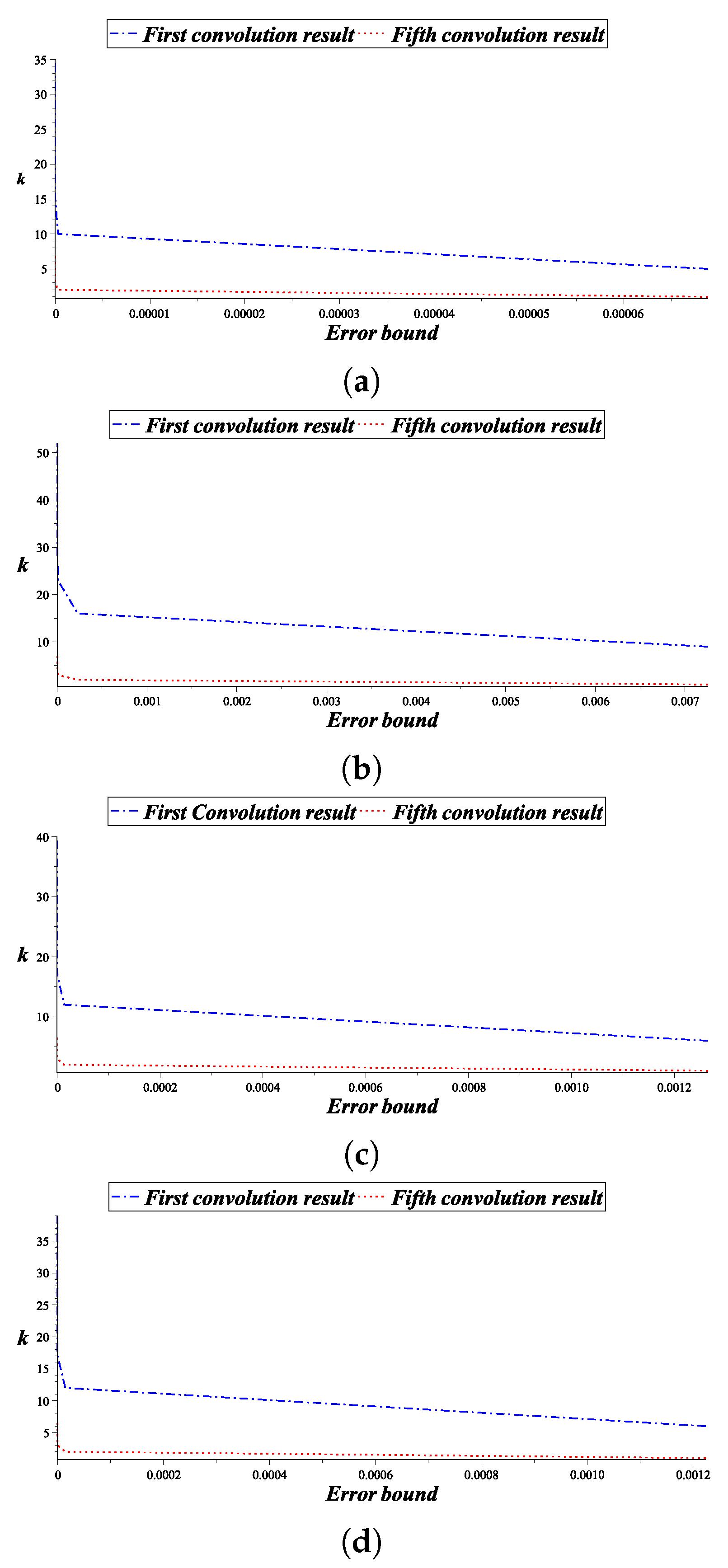
Remark 1.

In this technique $D_{k_0}$ for $k_0=1$ is equal to δ defined in [21]. Please note that in [21], if $\delta >1$ then error bounds cannot be computed. However, in the proposed technique, if we increase the value of $k_0$ until $D_{k_0}$ becomes less than one, so using this argument we can compute error bounds in each situation even though the value of δ becomes greater or equal to one.

Example 1.

Given initial polygon $p_i^0=p_i,i\in \mathbb{Z}$ with values $p_i^k,k\ge 1$ be interpreted recursively by the 2-point ternary approximating subdivision scheme [12] (i.e., $a_{0,0}=\frac{5}{6}$, $a_{0,1}=\frac{1}{6}$, $a_{1,0}=\frac{1}{2}$, $a_{1,1}=\frac{1}{2}$, $a_{2,0}=\frac{1}{6}$, $a_{2,1}=\frac{5}{6}$). For this ternary two point scheme ($N=2$), we have from (16)

$$D_{k_0}=\underset{j\in \mathsf{\Sigma }(k_0,2)}{sup}\left\{\sum _{m=0}^{\lfloor j/3^{k_0}\rfloor }|B_{m,j}^{k_0}|\right\}.$$

For $k_0=1$, we get

$$\begin{array}{ccc}{D}_1\hfill & =& \underset{j\in \mathsf{\Sigma }(1,2)}{sup}\left\{\sum _{m=0}^{\lfloor j/3\rfloor }|B_{m,j}^1|\right\}=\underset{j\in \{3,4,5\}}{sup}\left\{\sum _{m=0}^{\lfloor j/3\rfloor }|d_{j-3m}|\right\}.\hfill \end{array}$$

Using (3) and Lemma 1, we have $d={\{d_n\}}_{n=0}^5$ with $d_n=0$ for $n\ge 6$. Hence

$$\left\{d_0,d_1,d_2,d_3,d_4,d_5\right\}=\left\{\frac{1}{3},\frac{1}{3},\frac{1}{6},0,0,\frac{1}{6}\right\}.$$

Now consider

$$\begin{array}{ccc}{D}_1\hfill & =& sup\left\{\sum _{m=0}^{\lfloor 3/3\rfloor }|d_{3-3m}|,\sum _{m=0}^{\lfloor 4/3\rfloor }|d_{4-3m}|,\sum _{m=0}^{\lfloor 5/3\rfloor }|d_{5-3m}|\right\}.\hfill \end{array}$$

This implies

$$\begin{array}{ccc}{D}_1\hfill & =& sup\left\{|d_3|+|d_0|,|d_4|+|d_1|,|d_5|+|d_2|\right\}\hfill \\ & =& sup\left\{|0|+\left|\frac{1}{3}\right|,|0|+\left|\frac{1}{3}\right|,\left|\frac{1}{6}\right|+\left|\frac{1}{6}\right|\right\}=\frac{1}{3}.\hfill \end{array}$$

For $k_0=2$, we get

$$\begin{array}{ccc}{D}_2\hfill & =& \underset{j\in \mathsf{\Sigma }(2,2)}{sup}\left\{\sum _{m=0}^{\lfloor j/3^2\rfloor }|B_{m,j}^2|\right\}=\underset{j\in \{27,28,\dots ,35\}}{sup}\left\{\sum _{m=0}^{\lfloor j/9\rfloor }|B_{m,j}^2|\right\}\hfill \\ & =& \underset{j\in \{27,28,\dots ,35\}}{sup}\left\{\sum _{m=0}^{\lfloor j/9\rfloor }\left|\sum _{n=3m}^{\lfloor j/3\rfloor }{B}_{m,n}^1{B}_{n,j}^1\right|\right\}.\hfill \end{array}$$

This implies

$$\begin{array}{ccc}{D}_2\hfill & =& sup\left\{\sum _{m=0}^{\lfloor 27/9\rfloor }\right|\sum _{n=3m}^{\lfloor 27/3\rfloor }{B}_{m,n}^1{B}_{n,27}^1|,\sum _{m=0}^{\lfloor 28/9\rfloor }|\sum _{n=3m}^{\lfloor 28/3\rfloor }{B}_{m,n}^1{B}_{n,28}^1|,\sum _{m=0}^{\lfloor 29/9\rfloor }|\sum _{n=3m}^{\lfloor 29/3\rfloor }{B}_{m,n}^1{B}_{n,29}^1|,\hfill \\ & & \sum _{m=0}^{\lfloor 30/9\rfloor }\left|\sum _{n=3m}^{\lfloor 30/3\rfloor }{B}_{m,n}^1{B}_{n,30}^1\right|,\sum _{m=0}^{\lfloor 31/9\rfloor }\left|\sum _{n=3m}^{\lfloor 31/3\rfloor }{B}_{m,n}^1{B}_{n,31}^1\right|,\sum _{m=0}^{\lfloor 32/9\rfloor }\left|\sum _{n=3m}^{\lfloor 32/3\rfloor }{B}_{m,n}^1{B}_{n,32}^1\right|,\hfill \\ & & \sum _{m=0}^{\lfloor 33/9\rfloor }\left|\sum _{n=3m}^{\lfloor 33/3\rfloor }{B}_{m,n}^1{B}_{n,33}^1\right|,\sum _{m=0}^{\lfloor 34/9\rfloor }\left|\sum _{n=3m}^{\lfloor 34/3\rfloor }{B}_{m,n}^1{B}_{n,34}^1\right|,\sum _{m=0}^{\lfloor 35/9\rfloor }\left|\sum _{n=3m}^{\lfloor 35/3\rfloor }{B}_{m,n}^1{B}_{n,35}^1\right|\}.\hfill \end{array}$$

This further implies

$$\begin{array}{ccc}{D}_2\hfill & =& sup\left\{{\chi }_1,{\chi }_2,{\chi }_3,{\chi }_4,{\chi }_5,{\chi }_6,{\chi }_7,{\chi }_8,{\chi }_9\right\},\hfill \end{array}$$

where

$$\begin{array}{ccc}{\chi }_1\hfill & =& |d_0{d}_{27}+d_1{d}_{24}+d_2{d}_{21}+d_3{d}_{18}+d_4{d}_{15}+d_5{d}_{12}+d_6{d}_9+d_7{d}_6+d_8{d}_3+d_9{d}_0|+|d_0{d}_{18}\hfill \\ & & +d_1{d}_{15}+d_2{d}_{12}+d_3{d}_9+d_4{d}_6+d_5{d}_3+d_6{d}_0|+|d_0{d}_9+d_1{d}_6+d_2{d}_3+d_3{d}_0|+|d_0{d}_0|,\hfill \end{array}$$

$$\begin{array}{ccc}{\chi }_2\hfill & =& |d_0{d}_{28}+d_1{d}_{25}+d_2{d}_{22}+d_3{d}_{19}+d_4{d}_{16}+d_5{d}_{13}+d_6{d}_{10}+d_7{d}_7+d_8{d}_4+d_9{d}_1|+|d_0{d}_{19}\hfill \\ & & +d_1{d}_{16}+d_2{d}_{13}+d_3{d}_{10}+d_4{d}_7+d_5{d}_4+d_6{d}_1|+|d_0{d}_{10}+d_1{d}_7+d_2{d}_4+d_3{d}_1|+|d_0{d}_1|,\hfill \end{array}$$

$$\begin{array}{ccc}{\chi }_3\hfill & =& |d_0{d}_{29}+d_1{d}_{26}+d_2{d}_{23}+d_3{d}_{20}+d_4{d}_{17}+d_5{d}_{14}+d_6{d}_{11}+d_7{d}_8+d_8{d}_5+d_9{d}_2|+|d_0{d}_{20}\hfill \\ & & +d_1{d}_{17}+d_2{d}_{14}+d_3{d}_{11}+d_4{d}_8+d_5{d}_5+d_6{d}_2|+|d_0{d}_{11}+d_1{d}_8+d_2{d}_5+d_3{d}_2|+|d_0{d}_2|,\hfill \end{array}$$

$$\begin{array}{ccc}{\chi }_4\hfill & =& |d_0{d}_{30}+d_1{d}_{27}+d_2{d}_{24}+d_3{d}_{21}+d_4{d}_{18}+d_5{d}_{15}+d_6{d}_{12}+d_7{d}_9+d_8{d}_6+d_9{d}_3+d_{10}{d}_0|\hfill \\ & & +|d_0{d}_{21}+d_1{d}_{18}+d_2{d}_{15}+d_3{d}_{12}+d_4{d}_9+d_5{d}_6+d_6{d}_3+d_7{d}_0|+|d_0{d}_{12}+d_1{d}_9+d_2{d}_6\hfill \\ & & +d_3{d}_3+d_4{d}_0|+|d_0{d}_3+d_1{d}_0|,\hfill \end{array}$$

$$\begin{array}{ccc}{\chi }_5\hfill & =& |d_0{d}_{31}+d_1{d}_{28}+d_2{d}_{25}+d_3{d}_{22}+d_4{d}_{19}+d_5{d}_{16}+d_6{d}_{13}+d_7{d}_{10}+d_8{d}_7+d_9{d}_4+d_{10}{d}_1|\hfill \\ & & +|d_0{d}_{22}+d_1{d}_{19}+d_2{d}_{16}+d_3{d}_{13}+d_4{d}_{10}+d_5{d}_7+d_6{d}_4+d_7{d}_1|+|d_0{d}_{13}+d_1{d}_{10}+d_2{d}_7\hfill \\ & & +d_3{d}_4+d_4{d}_1|+|d_0{d}_4+d_1{d}_1|,\hfill \end{array}$$

$$\begin{array}{ccc}{\chi }_6\hfill & =& |d_0{d}_{32}+d_1{d}_{29}+d_2{d}_{26}+d_3{d}_{23}+d_4{d}_{20}+d_5{d}_{17}+d_6{d}_{14}+d_7{d}_{11}+d_8{d}_8+d_9{d}_5+d_{10}{d}_2|\hfill \\ & & +|d_0{d}_{23}+d_1{d}_{20}+d_2{d}_{17}+d_3{d}_{14}+d_4{d}_{11}+d_5{d}_8+d_6{d}_5+d_7{d}_2|+|d_0{d}_{14}+d_1{d}_{11}+d_2{d}_8\hfill \\ & & +d_3{d}_5+d_4{d}_2|+|d_0{d}_5+d_1{d}_2|,\hfill \end{array}$$

$$\begin{array}{ccc}{\chi }_7\hfill & =& |d_0{d}_{33}+d_1{d}_{30}+d_2{d}_{27}+d_3{d}_{24}+d_4{d}_{21}+d_5{d}_{18}+d_6{d}_{15}+d_7{d}_{12}+d_8{d}_9+d_9{d}_6+d_{10}{d}_3\hfill \\ & & +d_{11}{d}_0|+|d_0{d}_{24}+d_1{d}_{21}+d_2{d}_{18}+d_3{d}_{15}+d_4{d}_{12}+d_5{d}_9+d_6{d}_6+d_7{d}_3+d_8{d}_0|+|d_0{d}_{15}\hfill \\ & & +d_1{d}_{12}+d_2{d}_9+d_3{d}_6+d_4{d}_3+d_5{d}_0|+|d_0{d}_6+d_1{d}_3+d_2{d}_0|,\hfill \end{array}$$

$$\begin{array}{ccc}{\chi }_8\hfill & =& |d_0{d}_{34}+d_1{d}_{31}+d_2{d}_{28}+d_3{d}_{25}+d_4{d}_{22}+d_5{d}_{19}+d_6{d}_{16}+d_7{d}_{13}+d_8{d}_{10}+d_9{d}_7+d_{10}{d}_4\hfill \\ & & +d_{11}{d}_1|+|d_0{d}_{25}+d_1{d}_{22}+d_2{d}_{19}+d_3{d}_{16}+d_4{d}_{13}+d_5{d}_{10}+d_6{d}_7+d_7{d}_4+d_8{d}_1|+|d_0{d}_{16}\hfill \\ & & +d_1{d}_{13}+d_2{d}_{10}+d_3{d}_7+d_4{d}_4+d_5{d}_1|+|d_0{d}_7+d_1{d}_4+d_2{d}_1|,\hfill \end{array}$$

$$\begin{array}{ccc}{\chi }_9\hfill & =& |d_0{d}_{35}+d_1{d}_{32}+d_2{d}_{29}+d_3{d}_{26}+d_4{d}_{23}+d_5{d}_{20}+d_6{d}_{17}+d_7{d}_{14}+d_8{d}_{11}+d_9{d}_8+d_{10}{d}_5\hfill \\ & & +d_{11}{d}_2|+|d_0{d}_{26}+d_1{d}_{23}+d_2{d}_{20}+d_3{d}_{17}+d_4{d}_{14}+d_5{d}_{11}+d_6{d}_8+d_7{d}_5+d_8{d}_2|+|d_0{d}_{17}\hfill \\ & & +d_1{d}_{14}+d_2{d}_{11}+d_3{d}_8+d_4{d}_5+d_5{d}_2|+|d_0{d}_8+d_1{d}_5+d_2{d}_2\left|\right\}.\hfill \end{array}$$

Since $d_i=0$, for all $i>5$, so

$$\begin{array}{ccc}{D}_2\hfill & =& sup\{0+|d_5{d}_3|+|d_2{d}_3+d_3{d}_0|+|d_0{d}_0|,0+|d_5{d}_4|+|d_2{d}_4+d_3{d}_1|+|d_0{d}_1|,0+|d_5{d}_5|\hfill \\ & & +|d_2{d}_5+d_3{d}_2|+|d_0{d}_2|,0+0+|d_3{d}_3+d_4{d}_0|+|d_0{d}_3+d_1{d}_0|,0+0+|d_3{d}_4+d_4{d}_1|\hfill \\ & & +|d_0{d}_4+d_1{d}_1|,0+0+|d_3{d}_5+d_4{d}_2|+|d_0{d}_5+d_1{d}_2|,0+0+|d_4{d}_3+d_5{d}_0|+|d_1{d}_3+d_2{d}_0|,\hfill \\ & & 0+0+|d_4{d}_4+d_5{d}_1|+|d_1{d}_4+d_2{d}_1|,0+0+|d_4{d}_5+d_5{d}_2|+|d_1{d}_5+d_2{d}_2|\}.\hfill \end{array}$$

This further implies

$$\begin{array}{ccc}{D}_2\hfill & =& sup\left\{\frac{1}{9},\frac{1}{9},\frac{1}{9},\frac{1}{9},\frac{1}{9},\frac{1}{9},\frac{1}{9},\frac{1}{9},\frac{1}{9}\right\}=\frac{1}{9}.\hfill \end{array}$$

Similarly, we can compute the values of $D_{k_0},k_0\ge 3$. For convenience, we have computed the values up to $k_0=5$, which are shown in Table 1. Its subdivision depth k (level of iterations) is computed by using Theorem 3 at different values of $D_{k_0},k_0\ge 1$ which are given in

Table 2. Subdivision depth of 2-point approximating ternary subdivision curves.

${\mathit{D}}_{{\mathit{k}}_0}$/$\mathit{ϵ}$	$6.88\times {10}^{-5}$	$2.83\times {10}^{-7}$	$1.16\times {10}^{-9}$	$4.79\times {10}^{-12}$	$1.97\times {10}^{-14}$	$8.12\times {10}^{-17}$	$3.34\times {10}^{-19}$
$D_1=\delta$	5	10	15	20	25	30	35
$D_2$	3	5	8	10	13	15	18
$D_3$	2	3	5	7	8	10	12
$D_4$	1	2	4	5	6	7	9
$D_5$	1	2	3	4	5	6	7

.

From this table, we observed that as $k_0$ increases subdivision depth decreases. This shows that the less subdivision depth can be obtained by using proposed technique. In other words, we need fewer iteration to get optimal subdivision depth as compared to the technique given in [21] (which is denoted by $\delta$). For example, by [21], it needs thirty five iterations to obtain error tolerance $ϵ=3.34\times {10}^{-19}$ but using our technique, it needs only seven iterations corresponding to $D_5$. The comparison of first and fifth convolution results is shown in Figure 1a.

Example 2.

Consider the 3-point interpolating subdivision scheme [30] with $b=0.2778,a=b-\frac{1}{3}.$ Its subdivision depths k for $D_{k_0},k_0\ge 1$ (see, Table 1) are computed by using Theorem 3, which are shown in

Table 3. Subdivision depth of 3-point interpolating ternary subdivision curves.

${\mathit{D}}_{{\mathit{k}}_0}$/$\mathit{ϵ}$	$1.38\times {10}^{-3}$	$2.81\times {10}^{-5}$	$5.73\times {10}^{-7}$	$1.16\times {10}^{-8}$	$2.37\times {10}^{-10}$	$4.83\times {10}^{-12}$	$9.84\times {10}^{-14}$
$D_1=\delta$	8	15	21	28	34	41	48
$D_2$	3	6	9	12	14	17	20
$D_3$	2	4	5	7	9	11	12
$D_4$	1	3	4	5	6	8	9
$D_5$	1	2	3	4	5	6	7

and in graphical sense shown in Figure 1b.

Example 3.

Given initial control polygon $p_i^0=p_i,i\in \mathbb{Z}$ with values $p_i^k,k\ge 1$ be illustrated recursively by the ternary 4-point approximating scheme [8].

Its subdivision depth k for $D_{k_0},k_0\ge 1$ are given in

Table 4. Subdivision depth of 4-point approximating ternary subdivision curves.

${\mathit{D}}_{{\mathit{k}}_0}$/$\mathit{ϵ}$	$1.26\times {10}^{-3}$	$1.35\times {10}^{-5}$	$1.45\times {10}^{-7}$	$1.56\times {10}^{-9}$	$1.67\times {10}^{-11}$	$1.79\times {10}^{-13}$	$1.92\times {10}^{-15}$
$D_1=\delta$	6	12	17	23	28	34	40
$D_2$	3	5	8	11	13	16	18
$D_3$	2	3	5	7	8	10	12
$D_4$	1	3	4	5	6	8	9
$D_5$	1	2	3	4	5	6	7

. It is also demonstrated with the help of Figure 1c.

Example 4.

Given $p_i^0=p_i,i\in \mathbb{Z}$ be the initial polygon and for all positive integers we have the values $p_i^k$ be specified recursively by ternary 4-point interpolating subdivision scheme [6] with parameter $w=\frac{1}{12}$.

Its subdivision depths for $D_{k_0},k_0\ge 1$ (see, Table 1) are given in

Table 5. Subdivision depth of 4-point interpolating ternary subdivision curves.

${\mathit{D}}_{{\mathit{k}}_0}$/$\mathit{ϵ}$	$1.22\times {10}^{-3}$	$1.47\times {10}^{-5}$	$1.78\times {10}^{-7}$	$2.16\times {10}^{-9}$	$2.61\times {10}^{-11}$	$3.15\times {10}^{-13}$	$3.81\times {10}^{-15}$
$D_1=\delta$	6	12	17	22	28	33	39
$D_2$	3	5	8	10	13	15	18
$D_3$	2	3	5	7	8	10	12
$D_4$	1	2	4	5	6	7	9
$D_5$	1	2	3	4	5	6	7

and its performance is shown in Figure 1d.

3. Preliminary Results for Bivariate Case

In this section, we generalize our representation of the 2-dimensional case to the 3-dimensional case. That is, we first focus our attention on generalizing the inequalities presented in Section 2.1 then we generalize the inequalities of Section 2.2 to compute subdivision depth of tensor product surfaces. For this, let $\{p_{i,j}^k;i,j\in \mathbb{Z}\}$ be the sequence of 3D points ${\mathbf{R}}^{\mathbf{N}}$, $\mathbf{N}\ge 3$ which are produced by the following tensor product of ternary scheme (1)

$$p_{3i+\alpha ,3j+\beta }^{k+1}=\sum _{r=0}^{N-1}\sum _{s=0}^{N-1}{a}_{\alpha ,r}{a}_{\beta ,s}{p}_{i+r,m+s}^k,\alpha ,\beta =0,1,2,$$

(20)

where $a_{\alpha ,r}$ satisfies (2).

Now we assign the coefficients $f={\{f_n\}}_{n\in \mathbb{N}}$ and $g={\{g_n\}}_{n\in \mathbb{N}}$, by using the same procedure of symbolization given in [21] i.e.,

$$\begin{array}{c}\left\{\begin{array}{c}{f}_{3r}=a_{0,N-r-1},\hfill \\ f_{3r+1}=a_{1,N-r-1},\hfill \\ f_{3r+2}=a_{2,N-r-1}r=0,\dots ,N-1.\hfill \\ g_{3s}=b_{0,N-s-1}\hfill \\ g_{3s+1}=b_{1,N-s-1}\hfill \\ g_{3s+2}=b_{2,N-s-1}s=0,\dots ,N-1.\hfill \end{array}\right.\hfill \end{array}$$

To achieve the goal, all that is needed is to make the set up given before Section 2.1 for the 3D case. Here we skip the unnecessary detail and directly go to the following results.

Lemma 3.

Let $u=u_{m,n}$ be the vector of finite length for bivariate case and $f={\{f_n\}}_{n=0}^{3N-1}$, $g={\{g_n\}}_{n=0}^{3N-1}$ with $f_n=g_n=0$ for $n\ge 3N$, then the following two dimensional $k_0$ convolutions are bounded by

$$\underset{i,j}{max}|u_{i,j}^{k_0}|\le F_{k_0}{G}_{k_0}\underset{m,n}{max}|u_{m,n}^0|,$$

where

$$F_{k_0}=\underset{i}{max}\left\{\sum _{m=0}^{\lfloor i/3^{k_0}\rfloor }|B_{m,i}^{k_0,f}|\right\}$$

and

$$G_{k_0}=\underset{j}{max}\left\{\sum _{n=0}^{\lfloor j/3^{k_0}\rfloor }|B_{n,j}^{k_0,g}|\right\}.$$

Proof. 

To prove the result, we start with the case of $k_0=1$ and $k_0=2$ convolutions and later on we analyze the general case.

Case $k_0=1$: Consider an arbitrary sequence of vectors $u_{i,j}$. Then we have

$$u_{i,j}^{k_0}={(u^{k_0-1;0}★fg)}_{i,j}=\sum _{m=0}^{\lfloor i/3\rfloor }\sum _{n=0}^{\lfloor j/3\rfloor }{u}_{m,n}^{k_0-1}{f}_{i-3m}{g}_{j-3n},$$

where we are taking $B_{m,i}^{1,f}=f_{i-3m}$ and $g_{j-3n}=B_{n,j}^{1,g}$ for arbitrary sequence f and g. Thus,

$$u_{i,j}^{k_0}={(u^{k_0-1;0}★fg)}_{i,j}=\sum _{m=0}^{\lfloor i/3\rfloor }\sum _{n=0}^{\lfloor j/3\rfloor }{u}_{m,n}^{k_0-1}{B}_{m,i}^{1,f}{B}_{n,j}^{1,g}.$$

This implies

$$\begin{array}{ccc}\underset{i,j}{max}|u_{i,j}^{k_0}|\hfill & =& \underset{i,j}{max}\left|{\displaystyle \sum _{m=0}^{\lfloor i/3\rfloor }}{\displaystyle \sum _{n=0}^{\lfloor j/3\rfloor }}{u}_{m,n}^{k_0-1}{B}_{m,i}^{1,f}{B}_{n,j}^{1,g}\right|,\hfill \\ & \le & \underset{i,j}{max}{\displaystyle \sum _{m=0}^{\lfloor i/3\rfloor }}{\displaystyle \sum _{n=0}^{\lfloor j/3\rfloor }}|B_{m,i}^{1,f}||B_{n,j}^{1,g}|\underset{m,n}{max}|u_{m,n}^{k_0-1}|.\hfill \end{array}$$

(21)

Consider

$$F_1=\underset{i}{max}\left\{\sum _{m=0}^{\lfloor i/3\rfloor }|B_{m,i}^{1,f}|\right\}$$

and

$$G_1=\underset{j}{max}\left\{\sum _{n=0}^{\lfloor j/3\rfloor }|B_{n,j}^{1,g}|\right\},$$

then from (21), we obtain

$$\underset{i,j}{max}|u_{i,j}^{k_0}|\le F_1{G}_1\underset{m,n}{max}|u_{m,n}^{k_0-1}|.$$

Case $k_0=2$: Now, after applying two time convolution, we obtain

$$u_{m,n}^{k_0-1}={(u^{k_0-2;0}★fg)}_{m,n}={((u^{k_0-1;0}★fg)★fg)}_{i,j}.$$

This implies

$$\begin{array}{ccc}{u}_{i,j}^{k_0-1}\hfill & =& \sum _{m=0}^{\lfloor i/3\rfloor }\sum _{n=0}^{\lfloor j/3\rfloor }{(u^{k_0-1;0}★fg)}_{i,j}{f}_{i-3m}{g}_{j-3n}.\hfill \end{array}$$

This leads to

$$\begin{array}{ccc}{u}_{i,j}^{k_0-1}\hfill & =& \sum _{m=0}^{\lfloor i/3\rfloor }\sum _{n=0}^{\lfloor j/3\rfloor }\left(\sum _{p=0}^{\lfloor m/3\rfloor }\sum _{s=0}^{\lfloor n/3\rfloor }{u}_{p,s}^{k_0-2}{f}_{m-3p}{g}_{n-3s}\right)f_{i-3m}{g}_{j-3n}.\hfill \end{array}$$

This again implies that

$$\begin{array}{ccc}{u}_{i,j}^{k_0-1}\hfill & =& \sum _{m=0}^{\lfloor i/3^2\rfloor }\sum _{n=0}^{\lfloor j/3^2\rfloor }{u}_{m,n}^{k_0-2}\sum _{r=3m}^{\lfloor i/3\rfloor }{f}_{r-3m}{f}_{i-3r}\sum _{q=3n}^{\lfloor j/3\rfloor }{g}_{q-3n}{g}_{j-3q}.\hfill \end{array}$$

Further implies

$$\begin{array}{ccc}{u}_{i,j}^{k_0-1}\hfill & =& \sum _{m=0}^{\lfloor i/3^2\rfloor }\sum _{n=0}^{\lfloor j/3^2\rfloor }{u}_{m,n}^{k_0-2}\sum _{r=3m}^{\lfloor i/3\rfloor }{B}_{m,r}^{1,f}{B}_{r,i}^{1,f}\sum _{q=3n}^{\lfloor j/3\rfloor }{B}_{n,q}^{1,g}{B}_{q,j}^{1,g}.\hfill \end{array}$$

Furthermore

$$u_{i,j}^{k_0}=\sum _{m=0}^{\lfloor i/3^2\rfloor }\sum _{n=0}^{\lfloor j/3^2\rfloor }{u}_{m,n}^{k_0-2}{B}_{m,i}^{2,f}{B}_{n,j}^{2,g}.$$

Now

$$\begin{array}{ccc}\underset{i,j}{max}\left|u_{i,j}^{k_0}\right|\hfill & =& \underset{i,j}{max}\left|{\displaystyle \sum _{m=0}^{\lfloor i/3^2\rfloor }}{\displaystyle \sum _{n=0}^{\lfloor j/3^2\rfloor }}{u}_{m,n}^{k_0-2}{B}_{m,i}^{2,f}{B}_{n,j}^{2,g}\right|,\hfill \\ & \le & \underset{i,j}{max}{\displaystyle \sum _{m=0}^{\lfloor i/3^2\rfloor }}{\displaystyle \sum _{n=0}^{\lfloor j/3^2\rfloor }}\left|B_{m,i}^{2,f}\right|\left|B_{n,j}^{2,g}\right|\underset{m,n}{max}\left|u_{m,n}^{k_0-2}\right|.\hfill \end{array}$$

(22)

Consider

$$F_2=\underset{i}{max}\left\{\sum _{m=0}^{\lfloor i/3^2\rfloor }\left|B_{m,i}^{2,f}\right|\right\}$$

and

$$G_2=\underset{j}{max}\left\{\sum _{n=0}^{\lfloor j/3^2\rfloor }\left|B_{n,j}^{2,g}\right|\right\},$$

then we obtain from (22)

$$\underset{i,j}{max}|u_{i,j}^{k_0}|\le F_2{G}_2\underset{m,n}{max}|u_{m,n}^{k_0-2}|.$$

By the same strategy, we get the following reformulations for $k_0$-th convolution

$$\begin{array}{ccc}{u}_{i,j}^{k_0}\hfill & =& {(u^{k_0-k_0;0}★fg)}_{m,n}={(\dots (((u^{k_0-1;0}★fg)★fg)★\dots ★fg)★fg)}_{i,j}.\hfill \end{array}$$

This implies

$$\begin{array}{ccc}{u}_{i,j}^{k_0}\hfill & =& \sum _{m=0}^{\lfloor i/3^{k_0}\rfloor }\sum _{n=0}^{\lfloor j/3^{k_0}\rfloor }{u}_{m,n}^{0;0}{B}_{m,i}^{k_0,f}{B}_{n,j}^{k_0,g}=\sum _{m=0}^{\lfloor i/3^{k_0}\rfloor }\sum _{n=0}^{\lfloor j/3^{k_0}\rfloor }{u}_{m,n}^0{B}_{m,i}^{k_0,f}{B}_{n,j}^{k_0,g},\hfill \end{array}$$

where

$$B_{m,i}^{k_0,f}=\sum _{p=3m}^{\lfloor i/3^{k_0}-1\rfloor }{B}_{m,p}^{k_0-1,f}{B}_{p,i}^{k_0-1,f}$$

and

$$B_{n,j}^{k_0,g}=\sum _{r=3n}^{\lfloor j/3^{k_0}-1\rfloor }{B}_{n,s}^{k_0-1,g}{B}_{n,j}^{k_0-1,g}.$$

Thus,

$$\begin{array}{ccc}\underset{i,j}{max}|u_{i,j}^{k_0}|\hfill & =& \underset{i,j}{max}\left|{\displaystyle \sum _{m=0}^{\lfloor i/3^{k_0}\rfloor }}{\displaystyle \sum _{n=0}^{\lfloor j/3^{k_0}\rfloor }}{u}_{m,n}^0{B}_{m,i}^{k_0,f}{B}_{n,j}^{k_0,g}\right|,\hfill \\ & \le & \underset{i,j}{max}{\displaystyle \sum _{m=0}^{\lfloor i/3^{k_0}\rfloor }}{\displaystyle \sum _{n=0}^{\lfloor j/3^{k_0}\rfloor }}\left|B_{m,i}^{k_0,f}\right|\left|B_{n,j}^{k_0,g}\right|\underset{m,n}{max}\left|u_{m,n}^0\right|.\hfill \end{array}$$

(23)

Now consider

$$F_{k_0}=\underset{i}{max}\left\{\sum _{m=0}^{\lfloor i/3^{k_0}\rfloor }|B_{m,i}^{k_0,f}|\right\}=\underset{i\in \mathsf{\Sigma }(k_0,N)}{max}\left\{\sum _{m=0}^{\lfloor i/3^{k_0}\rfloor }|B_{m,i}^{k_0,f}|\right\}$$

(24)

and

$$G_{k_0}=\underset{j}{max}\left\{\sum _{n=0}^{\lfloor j/3^{k_0}\rfloor }|B_{n,j}^{k_0,g}|\right\}=\underset{j\in \mathsf{\Sigma }(k_0,N)}{max}\left\{\sum _{n=0}^{\lfloor j/3^{k_0}\rfloor }|B_{n,j}^{k_0,g}|\right\},$$

(25)

then, from (23), we obtain

$$\underset{i,j}{max}|u_{i,j}^{k_0}|\le F_{k_0}{G}_{k_0}\underset{m,n}{max}|u_{m,n}^0|,$$

where

$$\underset{i,j}{max}\left\{\sum _{m=0}^{\lfloor i/3^{k_0}\rfloor }\sum _{n=0}^{\lfloor j/3^{k_0}\rfloor }|B_{m,i}^{k_0,f}||B_{n,j}^{k_0,g}|\right\}=\underset{i,j\in \mathsf{\Sigma }(k_0,N)}{max}\left\{\sum _{m=0}^{\lfloor i/3^{k_0}\rfloor }\sum _{n=0}^{\lfloor j/3^{k_0}\rfloor }|B_{m,i}^{k_0,f}||B_{n,j}^{k_0,g}|\right\}.$$

□

3.1. Subdivision Depth for Ternary Subdivision Surfaces

In this section, we first compute error bounds for subdivision surfaces. Secondly, we use these error bounds to compute subdivision depths by using the methodology given in [21].

Theorem 4.

Consider the initial control polygon $p_{i,j}^0,i,j\in \mathbb{Z}$ and the values $p_{i,j}^k,k\ge 0$, recursively defined by (20) together with (2). Also $P^k$ be the representation of polygon at the points $\{p_{i,j}^k\}$. Then after two consecutive iterations k and $k+1$ the error bounds is given as follows

$$\begin{array}{c}\parallel P^{k+1}-P^k{\parallel }_{\infty }\le \left(\lambda {\beta }_1+\tau {\beta }_2+\mu {\beta }_3\right){(F_{k_0}{G}_{k_0})}^k,\hfill \end{array}$$

where $F_{k_0},G_{k_0},k_0\ge 1$ defined in (24) and (25), ${\beta }_t={max}_{i,j}\parallel {▵}_{i,j,t}^0\parallel ,t=1,2,3,$

$${▵}_{i,j,1}^k=p_{i+1,j}^k-p_{i,j}^k,{▵}_{i,j,2}^k=p_{i,j+1}^k-p_{i,j}^k,{▵}_{i,j,3}^k=p_{i+1,j+1}^k-p_{i,j+1}^k,$$

where λ, τ and μ are defined in [21].

Proof. 

See in [21]. □

Theorem 5.

Let a limit surface $P^{\infty }$ be linked with the subdivision iterative process, then under the same conditions used in Theorem 4 the following inequality hold

$$\parallel P^{\infty }-P^k{\parallel }_{\infty }\le (\lambda {\beta }_1+\tau {\beta }_2+\mu {\beta }_3)\left(\frac{{(F_{k_0}{G}_{k_0})}^k}{1-F_{k_0}{G}_{k_0}}\right),$$

where $k_0\ge 1$ is a natural number, such that $F_{k_0}{G}_{k_0}<1$.

Proof. 

See in [21]. □

Remark 2.

Here $F_1{G}_1$ is also equal to δ which is defined in [21].

Theorem 6.

Let k be subdivision depth and let ${\nabla }^k$ be the error bound between ternary subdivision surface $P^{\infty }$ and its k-level control polygon $P^k$. For arbitrary $ϵ>0$, if

$$k\ge lo{g}_{(F_{k_0}{G}_{k_0})}\left(\frac{ϵ(1-F_{k_0}{G}_{k_0})}{\lambda {\beta }_1+\tau {\beta }_2+\mu {\beta }_3}\right),$$

(26)

then ${\nabla }^k\le ϵ$.

Proof. 

Let ${\nabla }^k$ be the distance between limit surface $P^{\infty }$ and control polygon $P^k$ at k-th level defined in Theorem 5, such that

$${\nabla }^k={\parallel P^{\infty }-P^k\parallel }_{\infty }\le (\lambda {\beta }_1+\tau {\beta }_2+\mu {\beta }_3)\left(\frac{{(F_{k_0}{G}_{k_0})}^k}{1-F_{k_0}{G}_{k_0}}\right).$$

To obtain given tolerance $ϵ>0$, consider

$$(\lambda {\beta }_1+\tau {\beta }_2+\mu {\beta }_3)\left(\frac{{(F_{k_0}{G}_{k_0})}^k}{1-F_{k_0}{G}_{k_0}}\right)\le ϵ,$$

which implies

$$\left(\frac{\lambda {\beta }_1+\tau {\beta }_2+\mu {\beta }_3}{ϵ(1-F_{k_0}{G}_{k_0})}\right)\le {({(F_{k_0}{G}_{k_0})}^{-1})}^k.$$

Now taking logarithm, we have

$$\begin{array}{c}k\ge \frac{log\left(\frac{\lambda {\beta }_1+\tau {\beta }_2+\mu {\beta }_3}{ϵ(1-F_{k_0}{G}_{k_0})}\right)}{log{(F_{k_0}{G}_{k_0})}^{-1}}=\frac{log\left(\frac{\lambda {\beta }_1+\tau {\beta }_2+\mu {\beta }_3}{ϵ(1-F_{k_0}{G}_{k_0})}\right)}{-log(F_{k_0}{G}_{k_0})}=-{log}_{(F_{k_0}{G}_{k_0})}\left(\frac{\lambda {\beta }_1+\tau {\beta }_2+\mu {\beta }_3}{ϵ(1-F_{k_0}{G}_{k_0})}\right),\hfill \end{array}$$

which implies

$$k\ge {log}_{(F_{k_0}{G}_{k_0})}{\left(\frac{\lambda {\beta }_1+\tau {\beta }_2+\mu {\beta }_3}{ϵ(1-F_{k_0}{G}_{k_0})}\right)}^{-1},$$

which further implies

$$k\ge {log}_{(F_{k_0}{G}_{k_0})}\left(\frac{ϵ(1-F_{k_0}{G}_{k_0})}{\lambda {\beta }_1+\tau {\beta }_2+\mu {\beta }_3}\right),$$

then ${\nabla }^k\le ϵ$. This completes the proof. □

3.2. Application for Bivariate Case

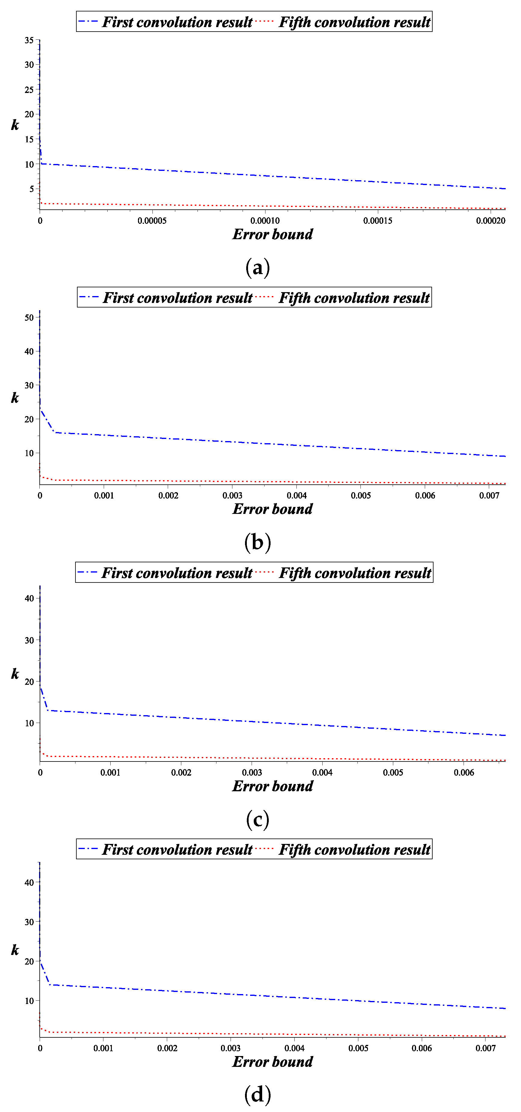
Here, we present some numerical examples to compute subdivision depth for subdivision surfaces. The associated constants $F_{k_0}{G}_{k_0},k_0\ge 1$ for some ternary subdivision surfaces by using (24) and (25) are shown in

Table 6. Associated constants of ternary subdivision surfaces.

Scheme/${\mathit{F}}_{{\mathit{k}}_0}{\mathit{G}}_{{\mathit{k}}_0}$	${\mathit{F}}_1{\mathit{G}}_1$	${\mathit{F}}_2{\mathit{G}}_2$	${\mathit{F}}_3{\mathit{G}}_3$	${\mathit{F}}_4{\mathit{G}}_4$	${\mathit{F}}_5{\mathit{G}}_5$
2-point scheme [12]	0.333333	0.111111	0.037037	0.012346	0.004115
3-point scheme [30]	0.61716	0.304535	0.145678	0.068303	0.031622
4-point scheme [8]	0.505401	0.233098	0.096089	0.040774	0.016958
4-point scheme [6]	0.54321	0.228729	0.10226	0.047435	0.021475

. We see that the values of $F_{k_0}{G}_{k_0}$ decrease with the increase of $k_0$. This is the main advantage of our proposed approach.

Example 5.

Given the initial polygon $p_{i,j}^0=p_{i,j},i,j\in \mathbb{Z}$ with values $p_{i,j}^k,k\ge 1$ be frequent explanation in [12], then the subdivision depths for $F_{k_0}{G}_{k_0},k_0\ge 1$ by using Theorem 6 are shown in

Table 7. Subdivision depth of 2-point ternary subdivision surfaces.

${\mathit{F}}_{{\mathit{k}}_0}{\mathit{G}}_{{\mathit{k}}_0}$/$\mathit{ϵ}$	$2.06\times {10}^{-3}$	$8.5\times {10}^{-7}$	$3.49\times {10}^{-9}$	$1.43\times {10}^{-11}$	$5.92\times {10}^{-14}$	$2.43\times {10}^{-16}$	$1.003\times {10}^{-18}$
$F_1{G}_1$	5	10	15	20	25	30	35
$F_2{G}_2$	3	5	8	10	13	15	18
$F_3{G}_3$	1	3	5	6	8	10	11
$F_4{G}_4$	1	2	4	5	6	7	9
$F_5{G}_5$	1	2	3	4	5	6	7

. The first and fifth convolution comparison results are shown in Figure 2a.

Example 6.

Given control polygon $p_{i,j}^0=p_{i,j},i,j\in \mathbb{Z}$ with the values $p_{i,j}^k$ for all positive integers be illustrated by the tensor product of the scheme demonstrated in [30], then the subdivision depths for $F_{k_0}{G}_{k_0},k_0\ge 1$ by using Theorem 6 are shown in

Table 8. Subdivision depth of 3-point ternary subdivision surfaces.

${\mathit{F}}_{{\mathit{k}}_0}{\mathit{G}}_{{\mathit{k}}_0}$/$\mathit{ϵ}$	$7.25\times {10}^{-3}$	$2.29\times {10}^{-4}$	$7.25\times {10}^{-6}$	$2.29\times {10}^{-7}$	$7.25\times {10}^{-9}$	$2.29\times {10}^{-10}$	$7.25\times {10}^{-12}$
$F_1{G}_1$	9	16	23	31	38	45	52
$F_2{G}_2$	3	6	9	12	15	18	21
$F_3{G}_3$	2	4	5	7	9	11	13
$F_4{G}_4$	1	3	4	5	6	8	9
$F_5{G}_5$	1	2	3	4	5	6	7

and in the sense of graphical structure these results are shown in Figure 2b.

Example 7.

Given an initial control polygon $p_{i,j}^0=p_{i,j},i,j\in \mathbb{Z}$ with the values $p_{i,j}^k,k\ge 1$ be frequent explanation by the tensor product of the scheme presented in [8], then the subdivision depths for $F_{k_0}{G}_{k_0},k_0\ge 1$ by using Theorem 6 are shown in

Table 9. Subdivision depth of 4-point ternary subdivision surfaces.

${\mathit{F}}_{{\mathit{k}}_0}{\mathit{G}}_{{\mathit{k}}_0}$/$\mathit{ϵ}$	$6.59\times {10}^{-3}$	$1.11\times {10}^{-4}$	$1.18\times {10}^{-6}$	$3.21\times {10}^{-8}$	$5.45\times {10}^{-10}$	$9.24\times {10}^{-12}$	$1.56\times {10}^{-13}$
$F_1{G}_1$	7	13	19	25	31	37	43
$F_2{G}_2$	3	6	9	11	14	17	20
$F_3{G}_3$	2	4	5	7	9	10	12
$F_4{G}_4$	1	3	4	5	6	8	9
$F_5{G}_5$	1	2	3	4	5	6	7

and graphical results are presented in Figure 2c.

Example 8.

Given $p_{i,j}^0=p_{i,j},i,j\in \mathbb{Z}$ be the initial polygon with values $p_{i,j}^k,k\ge 1$ be illustrated by the tensor product of the scheme presented in [6] with $w=1/12$, then the subdivision depths for $F_{k_0}{G}_{k_0},k_0\ge 1$ are shown in

Table 10. Subdivision depth of 4-point ternary subdivision surfaces.

${\mathit{F}}_{{\mathit{k}}_0}{\mathit{G}}_{{\mathit{k}}_0}$/$\mathit{ϵ}$	$7.31\times {10}^{-3}$	$1.57\times {10}^{-4}$	$3.37\times {10}^{-6}$	$7.24\times {10}^{-8}$	$1.55\times {10}^{-9}$	$3.34\times {10}^{-11}$	$7.17\times {10}^{-13}$
$F_1{G}_1$	8	14	20	26	33	39	45
$F_2{G}_2$	3	5	8	11	13	16	18
$F_3{G}_3$	2	3	5	7	8	10	12
$F_4{G}_4$	1	3	4	5	6	8	9
$F_5{G}_5$	1	2	3	4	5	6	7

. Also demonstration of graphical view are given in Figure 2d.

4. Conclusions

We described a formula to find the sharp error bounds between the polygon at any stage and the limiting polygon of the subdivision scheme. In addition, we have achieved a computational formula of subdivision depth for ternary subdivision schemes by using the error bounds. Existing methods only work under the strong condition given in ([21], Equation (2.3)). In this paper, we relaxed the strict condition by convolving the mask of the schemes. Using our framework, we can get sharp bounds and subdivision depths by increasing the convolution steps. Ultimately, the suggested numerical method work when the other methods fail. In addition, extensive numerical experiments predict that if we have a prescribed error tolerance then a finer shape can be obtained by using fewer subdivision steps (i.e., depths). In the future, we will generalize our framework for higher arity (i.e., quaternary, quinary, and so on) schemes.