Global Behavior of an Arbitrary-Order Nonlinear Difference Equation with a Nonnegative Function

Abstract

Let $k,l$ be two integers with $k\ge 0$ and $l\ge 2$, c a real number greater than or equal to 1, and f a multivariable function satisfying $f(w_1,w_2,w_3,\cdots ,w_l)\ge 0$ when $w_1,w_2\ge 0$. We consider an arbitrary order nonlinear difference equation with the indicated function f: $z_{n+1}=\frac{c(z_n+z_{n-k})+(c-1)z_n{z}_{n-k}+cf(z_n,z_{n-k},w_3,\cdots ,w_l)}{z_n{z}_{n-k}+f(z_n,z_{n-k},w_3,\cdots ,w_l)+c},n\ge 0,$ where initial values $z_{-k},z_{-k+1},\cdots ,z_0$ are positive and $w_i,i\ge 3$, are arbitrary functions of $z_j,n-k\le j\le n$. We classify its solutions into three types with different asymptotic behaviors, and verify the global asymptotic stability of its positive equilibrium solution $\overline{z}=c$.

1. Introduction

Difference equations regard time as a discrete quantity, and are treated in mathematics as discrete dynamical systems. Examples include inflation and unemployment data, published once a month or once a year, which tells us an inverse correlation between inflation and unemployment. Difference equations are similar to differential equations, but the latter regard time as a continuous quantity and examples include continuous dynamical systems.

There are various ways of solving linear difference equations [1]. However, for nonlinear difference equations, properties of solutions, in various situations, can only be observed and conjectured by numerical simulations, and they are extremely difficult to verify rigorously in mathematical ways [2]. Global asymptotics of special functions also play key roles in formulating algebro-gemoetric solutions to soliton equations (see, e.g., [3,4]) and determining scattering data in matrix spectral problems (see, e.g., [5]). It is, therefore, fundamentally important to make qualitative analysis on nonlinear difference equations, particularly global behaviors, and this is the topic of the current study. There have been some related mathematical studies on rational difference equations in the literature (see, e.g., [6,7,8,9,10,11]).

In numerical mathematics, an iterative algorithm (see, e.g., [12]) to approximate a zero of a given function g reads

$$x_{n+1}=\frac{x_{n-1}g\left(x_n\right)-x_{n}g\left(x_{n-1}\right)}{g\left(x_n\right)-g\left(x_{n-1}\right)},n\ge 0.$$

(1)

An application of this algorithm to a quadratic function $g\left(x\right)=x^2-a,a>0$ gives a special rational difference equation

$$x_{n+1}=\frac{x_n{x}_{n-1}+a}{x_n+x_{n-1}},n\ge 0.$$

(2)

In this paper, we would like to consider a more general difference equation.

Let $k,l$ be two integers with $k\ge 0$ and $l\ge 2$, c a real number greater than or equal to 1, and f a multivariable function satisfying that

$$f(w_1,w_2,w_3,\cdots ,w_l)\ge 0,\mathrm{when}{w}_1,w_2\ge 0.$$

(3)

We would like to study a $(k+1)$th-order nonlinear difference equation involving an indicated function f:

$$z_{n+1}=\frac{c(z_n+z_{n-k})+(c-1)z_n{z}_{n-k}+cf(z_n,z_{n-k},w_3,\cdots ,w_l)}{z_n{z}_{n-k}+f(z_n,z_{n-k},w_3,\cdots ,w_l)+c},n\ge 0,$$

(4)

with positive initial values $z_{-k},z_{-k+1},\cdots ,z_0$ and $w_i,i\ge 3$, being arbitrary functions of $z_j,n-k\le j\le n$. Taking positive initial values and the property (3) guarantees positive solutions. It is direct to see that this difference Equation (4) possesses only one equilibrium: $\overline{z}=c$, among positive solutions. Upon taking a transformation

$$z_n=\frac{c}{y_n},n\ge -k,$$

(5)

we obtain an equivalent difference equation

$$y_{n+1}=\frac{c(y_n{y}_{n-k}+c)+f(c/y_n,c/y_{n-k})y_n{y}_{n-k}}{c(y_n+y_{n-k}+c-1)+f(c/y_n,c/y_{n-k})y_n{y}_{n-k}},n\ge 0,$$

(6)

where $f=f(w_1,w_2)$ is assumed. The positive equilibrium solution $\overline{z}=c$ of the difference Equation (4) becomes the positive equilibrium solution $\overline{y}=1$ of the transformed difference Equation (6).

A reduction with $c=1$ and $f=0$ yields the rational difference equation studied in [9,10]:

$$y_{n+1}=\frac{y_n{y}_{n-k}+1}{y_n+y_{n-k}},n\ge 0.$$

(7)

Introducing $x_n=\sqrt{a}{y}_n$ into (7) generates

$$x_{n+1}=\frac{x_n{x}_{n-k}+a}{x_n+x_{n-k}},n\ge 0,$$

(8)

where $a>0$. This resulting difference equation in the case of $k=1$ is exactly the numerical algorithm in (2).

In this paper, we would like to show that there are three solution categories for the nonlinear difference Equation (4). A characterization of oscillatory solutions will be made, and the global asymptotic stability properties of the positive equilibrium solution $\overline{z}=c$ will be verified. Finally, a few illustrative examples of solutions will be presented.

2. Global Behavior

2.1. Classification of Solutions

Immediately from the difference Equation (4), we can derive

$$z_{n+1}-c=\frac{(c-z_n)(z_{n-k}-c)}{z_n{z}_{n-k}+f(z_n,z_{n-k},w_3,\cdots ,w_l)+c},n\ge 0,$$

(9)

$$z_{n+1}-z_n=\frac{(c-z_n)[(z_n+1)z_{n-k}+f(z_n,z_{n-k},w_3,\cdots ,w_l)]}{z_n{z}_{n-k}+f(z_n,z_{n-k},w_3,\cdots ,w_l)+c},n\ge 0,$$

(10)

and

$$z_{n+1}-z_{n-k}=\frac{(c-z_{n-k})[(z_{n-k}+1)z_n+f(z_n,z_{n-k},w_3,\cdots ,w_l)]}{z_n{z}_{n-k}+f(z_n,z_{n-k},w_3,\cdots ,w_l)+c},n\ge 0.$$

(11)

Now from the equalities (10) and (11), we can easily get the following solution properties.

Proposition 1.

Let ${\left\{z_n\right\}}_{n=-k}^{\infty }$ be a solution to the nonlinear difference Equation (4). Then we have

$$z_{n+1}>z_{n}if{z}_n<c,and{z}_{n+1}<z_{n}if{z}_n>c,$$

(12)

and

$$z_{n+1}>z_{n-k}if{z}_{n-k}<c,and{z}_{n+1}<z_{n-k}if{z}_{n-k}>c,$$

(13)

where $n\ge 0$.

If we take $k=0$, then the nonlinear difference Equation (4) becomes a first-order difference equation

$$z_{n+1}=\frac{2c{z}_n+(c-1)z_n^2+cf(z_n,z_n,w_3,\cdots ,w_l)}{z_n^2+f(z_n,z_n,w_3,\cdots ,w_l)+c},n\ge 0.$$

(14)

On one hand, for $n\ge 0$, we have $z_{n+1}\le c$, since $-z_n^2+2c{z}_n\le c^2$. On the other hand, for $n\ge 1$, we have $z_{n+1}\ge z_n$, because $c+(c-1)z_n\ge z_n^2$, due to $z_n\le c$. Therefore, $z_n$ increases to c, when $n\to \infty$.

Generally, the equality (9) and the property (12) directly tell that there are three types of solutions to the higher-order nonlinear difference Equation (4) as follows.

Theorem 1

(Classification of solutions). Let $k\ge 1$. Suppose that ${\left\{z_n\right\}}_{n=-k}^{\infty }$ solves the $(k+1)$th-order nonlinear difference Equation (4) with a function f satisfying (3). Then it

(i) 

eventually equals c, more precisely $z_n=c,n\ge m$, which occurs when $z_m=c$ for some $m\ge 0$;

(ii) 

is eventually less than c, more precisely $z_n<z_{n+1}<c$, $n\ge m+k$, which occurs when $z_m,z_{m+1},\cdots ,z_{m+k}<c$ for some $m\ge -k$; or

(iii) 

oscillates about c with at most $k+1$ consecutive decreasing terms greater than c and at most k consecutive increasing terms less than c.

We point out that another situation that a solution of (4) is eventually greater than c does not occur, which is guaranteed by (9).

A solution ${\left\{z_n\right\}}_{n=-k}^{\infty }$ in the third type of solutions (iii) of Theorem 1 is called an oscillatory solution. For an oscillatory solution to the nonlinear difference Equation (4), we can verify its decreasing and increasing characteristics as follows.

Let $n_1,n_2\ge 0$ be two integers satisfying $n_1<n_2$. Based on (10), we can compute that

$$\begin{array}{cc}\hfill {\displaystyle z_{n_2}-z_{n_1}}& =(z_{n_2}-z_{n_1+1})+(z_{n_1+1}-z_{n_1})\hfill \\ & =\sum _{j=n_1+1}^{n_2-1}(z_{j+1}-z_j)+(z_{n_1+1}-z_{n_1})\hfill \\ & =D+(z_{n_1+1}-z_{n_1}),\hfill \end{array}$$

(15)

with D being defined by

$$D=\sum _{j=n_1+1}^{n_2-1}\frac{(c-z_j)[(z_j+1)z_{j-k}+f(z_j,z_{j-k},w_3,\cdots ,w_l)]}{z_j{z}_{j-k}+f(z_j,z_{j-k},w_3,\cdots ,w_l)+c},$$

(16)

where an empty sum is conventionally assumed to be 0. Now if $n_2=n_1+1$, the monotonicity follows from the solution property (12). Hence, we assume that $n_2\ge n_1+2$. Consider the case of $z_n>c,n_1\le n\le n_2$. Using the definition of D in (16), we know $D<0$, and so $z_{n_2}<z_{n_1}$, due to (15). Consider the case of $z_n<c,n_1\le n\le n_2$. Using the definition of D in (16), we know $D>0$, and so $z_{n_2}>z_{n_1}$, due to (15).

2.2. Global Asymptotic Stability

Please note that the $(k+1)$th-order nonlinear difference Equation (4) has the unique positive equilibrium solution $\overline{z}=c$.

Because a globally attractive equilibrium solution of a first-order difference equation cannot be unstable [13], the positive equilibrium solution $\overline{z}=c$ of the first-order difference Equation (14) is globally asymptotically stable. This is for the case of $k=0$ in the nonlinear difference Equation (4).

In what follows, we would like to establish the same result for the general case of $k\ge 1$. We can show the global asymptotic stability property of the positive equilibrium solution $\overline{z}=c$, by verifying the local asymptotic stability and the global attractivity, which imply the global asymptotic stability [2]. Instead, we are going to prove a strong negative feedback property [14], which guarantees the global asymptotic stability (see [15] for a generalization of the strong negative feedback property).

Theorem 2

(Global asymptotic stability). The positive equilibrium solution $\overline{z}=c$ of the $(k+1)$th-order nonlinear difference Equation (4) with a function f satisfying (3) is globally asymptotically stable.

Proof. 

Let $g_n=f(z_n,z_{n-k},w_3,\cdots ,w_l)$. Beginning with the nonlinear difference Equation (4), we can obtain by a direct computation:

$$\frac{c^2}{z_{n-k}}-z_{n+1}=\frac{(c-z_{n-k})[(c-1)z_n{z}_{n-k}+c{z}_{n-k}+c{g}_n+c^2]}{z_{n-k}[z_n{z}_{n-k}+g_n+c]},n\ge 0.$$

It now follows from this equality and the equality (11) that

$$\begin{array}{cc}\hfill & (z_{n-k}-z_{n+1})(\frac{c^2}{z_{n-k}}-z_{n+1})\hfill \\ \hfill =& -\frac{{(c-z_{n-k})}^2[z_n{z}_{n-k}+z_n+g_n][(c-1)z_n{z}_{n-k}+c{z}_{n-k}+c{g}_n+c^2]}{z_{n-k}{[z_n{z}_{n-k}+g_n+c]}^2},n\ge 0,\hfill \end{array}$$

which implies a strong negative feedback property:

$$(z_{n-k}-z_{n+1})(\frac{c^2}{z_{n-k}}-z_{n+1})\le 0,n\ge 0,$$

with equality for all $n\ge 0$ if and only if $z_n=c,n\ge -k$. Finally, by a stability theorem in [14] (Theorem 4 in [14]), the positive equilibrium solution $\overline{z}=c$ of the nonlinear difference Equation (4) is globally asymptotically stable. The proof is finished. □

2.3. Illustrative Examples

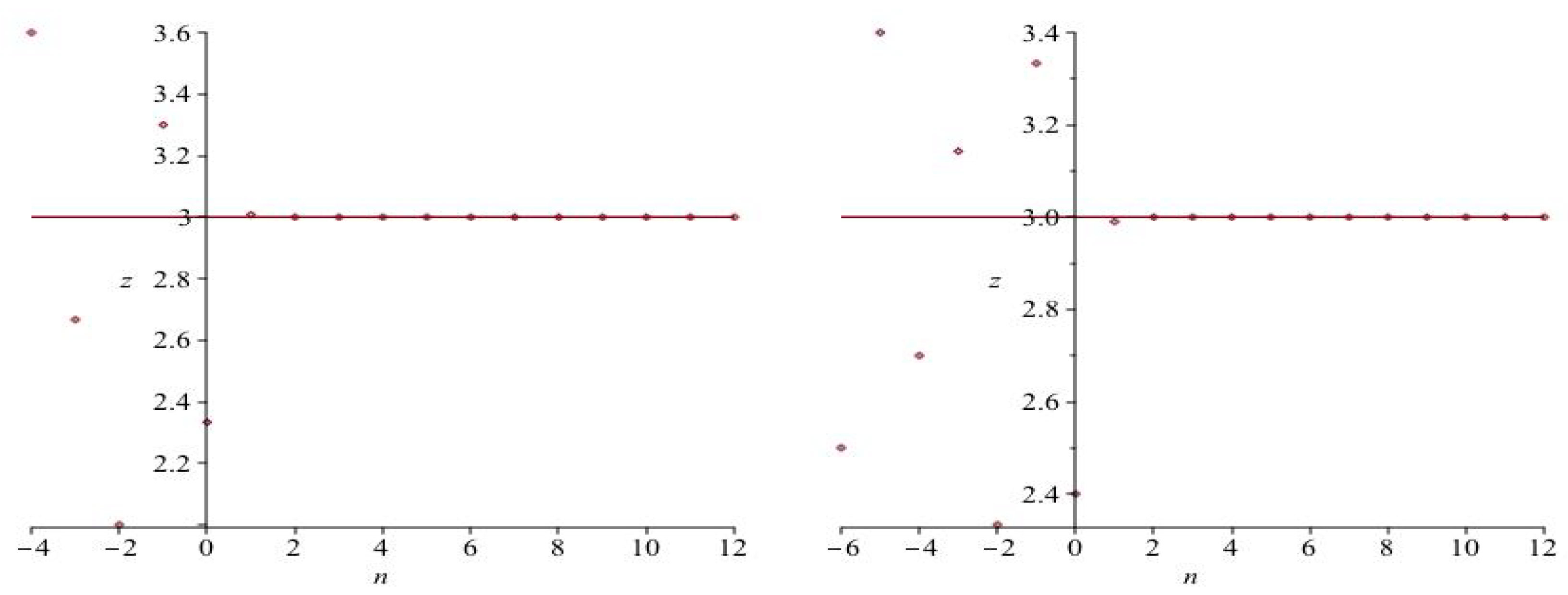
To illustrate the oscillation property and the global asymptotic stability in Theorems 1 and 2, we present two sets of specific examples associated with two special choices for c and f:

$$c=2,f(w_1,w_2)=w_1^2+2w_1{w}_2,$$

and

$$c=3,f(w_1,w_2)=3w_2+w_1{w}_2^2.$$

For the first choice, we take

$$k=3,z_{-3}=\frac{6}{5},z_{-2}=\frac{7}{3},z_{-1}=\frac{9}{7},z_0=\frac{8}{3},$$

and

$$k=5,z_{-5}=\frac{8}{7},z_{-4}=\frac{9}{5},z_{-3}=\frac{7}{3},z_{-2}=\frac{5}{3},z_{-1}=\frac{3}{2},z_0=\frac{5}{2}.$$

The two corresponding plots are displayed in Figure 1.

For the second choice, we take

$$k=4,z_{-4}=\frac{18}{5},z_{-3}=\frac{8}{3},z_{-2}=2,z_{-1}=\frac{33}{10},z_0=\frac{7}{3},$$

and

$$k=6,z_{-6}=\frac{5}{2},z_{-5}=\frac{17}{5},z_{-4}=\frac{27}{10},z_{-3}=\frac{22}{7},z_{-2}=\frac{7}{3},z_{-1}=\frac{10}{3},z_0=\frac{12}{5}.$$

The two corresponding plots are displayed in Figure 2.

From the four plot pictures, we see that the rate of convergence is excellent in every case.

3. Concluding Remarks

In this paper, we showed that there are three types of solutions to an arbitrary-order nonlinear difference equation involving a pretty arbitrary function. A decreasing and increasing characteristic of oscillatory solutions has been explored and the global asymptotic stability of the unique positive equilibrium solution has been verified.

We remark that if we take $c=1$ and $f=0$, Theorem 2 provides the result in [7] for $k=1$, the one in [8] for $k=2$ and the one in [10] for a general k. There have also been similar studies on global behaviors of polynomial difference equations (see, e.g., [16]) and rational difference equations or systems (see, e.g., [6,7,8,9,10,11,17]), and other recent studies on positive rational function solutions, called lump solutions, to both linear and nonlinear partial differential equations (see, e.g., [18,19]).

Let $k\ge 1$. Suppose that ${\left\{z_n\right\}}_{n=-k}^{\infty }$ is an oscillatory solution to the nonlinear difference Equation (4). We define

$$N_g=\left\{n\right|z_n>c\mathrm{and}n\ge 0\},N_l=\left\{n\right|z_n<c\mathrm{and}n\ge 0\}.$$

Because ${\left\{z_n\right\}}_{n=-k}^{\infty }$ is oscillatory, it follows directly from Theorem 1 that both $N_g$ and $N_l$ have infinitely many numbers. An interesting question is what kind of conditions on f will guarantee that $z_n$ is decreasing on $N_g$ and increasing on $N_l$.

References

- Batchelder, P.M. An Introduction to Linear Difference Equations; Dover Publications: New York, NY, USA, 1967. [Google Scholar]
- Kocic, V.L.; Ladas, G. Global Behavior of Nonlinear Difference Equations of Higher Order with Applications; Kluwer: Dordrecht, The Netherlands, 1993. [Google Scholar]
- Ma, W.X. Trigonal curves and algebro-geometric solutions to soliton hierarchies I. Proc. Roy. Soc. A 2017, 473, 20170232. [Google Scholar] [CrossRef] [PubMed]
- Ma, W.X. Trigonal curves and algebro-geometric solutions to soliton hierarchies II. Proc. Roy. Soc. A 2017, 473, 20170233. [Google Scholar] [CrossRef] [PubMed] [Green Version]
- Ma, W.X. The inverse scattering transform and soliton solutions of a combined modified Korteweg-de Vries equation. J. Math. Anal. Appl. 2019, 471, 796–811. [Google Scholar] [CrossRef]
- Camouzis, E.; Ladas, G.; Rodrigues, I.W.; Northshield, S. The rational recursive sequence . Comput. Math. Appl. 1994, 28, 37–43. [Google Scholar] [CrossRef] [Green Version]
- Li, X.; Zhu, D. Global asymptotic stability in a rational equation. J. Differ. Equ. Appl. 2003, 9, 833–839. [Google Scholar]
- Li, X.; Zhu, D. Two rational recursive sequences. Comput. Math. Appl. 2004, 47, 1487–1494. [Google Scholar] [CrossRef] [Green Version]
- Rhouma, M.B.H. The Fibonacci sequence modulo π, chaos and some rational recursive equations. J. Math. Anal. Appl. 2005, 310, 506–517. [Google Scholar] [CrossRef] [Green Version]
- Abu-Saris, R.; Çinar, C.; Yalçinkaya, I. On the asymptotic stability of xn+1 = (a + xnxn−k)/(xn + xn−k). Comput. Math. Appl. 2008, 56, 1172–1175. [Google Scholar] [CrossRef] [Green Version]
- Gelişken, A.; Çinar, C.; Kurbanli, A.S. On the asymptotic behavior and periodic nature of a difference equation with maximum. Comput. Math. Appl. 2010, 59, 898–902. [Google Scholar] [CrossRef] [Green Version]
- Ralston, A.; Rabinowitz, P. A First Course in Numerical Analysis; McGraw-Hill: New York, NY, USA, 1978. [Google Scholar]
- Sedaghat, H. The impossibility of unstable, globally attracting fixed points for continuous mappings of the line. Amer. Math. Mon. 1997, 104, 356–358. [Google Scholar] [CrossRef]
- Amleh, A.M.; Kruse, N.; Ladas, G. On a class of difference equations with strong negative feedback. J. Differ. Equ. Appl. 1999, 5, 497–515. [Google Scholar] [CrossRef]
- Kruse, N.; Nesemann, T. Global asymptotic stability in some discrete dynamical systems. J. Math. Anal. Appl. 1999, 235, 151–158. [Google Scholar] [CrossRef] [Green Version]
- Li, X.; Zhu, D. Global asymptotic stability for two recursive difference equations. Appl. Math. Comput. 2004, 150, 481–492. [Google Scholar] [CrossRef]
- Gümüş, M. The global asymptotic stability of a system of difference equations. J. Differ. Equ. Appl. 2018, 24, 976–991. [Google Scholar] [CrossRef]
- Ma, W.X. Lump and interaction solutions to linear PDEs in 2 + 1 dimensions via symbolic computation. Mod. Phys. Lett. B 2019, 33, 1950457. [Google Scholar] [CrossRef]
- Ma, W.X.; Zhou, Y. Lump solutions to nonlinear partial differential equations via Hirota bilinear forms. J. Diff. Equ. 2018, 264, 2633–2659. [Google Scholar] [CrossRef] [Green Version]
Figure 1.
Profiles of with and : (left), (right).
Figure 2.
© 2020 by the author. Licensee MDPI, Basel, Switzerland. This article is an open access article distributed under the terms and conditions of the Creative Commons Attribution (CC BY) license (http://creativecommons.org/licenses/by/4.0/).
Share and Cite
MDPI and ACS Style
Ma, W.-X. Global Behavior of an Arbitrary-Order Nonlinear Difference Equation with a Nonnegative Function. Mathematics 2020, 8, 825. https://doi.org/10.3390/math8050825
AMA Style
Ma W-X. Global Behavior of an Arbitrary-Order Nonlinear Difference Equation with a Nonnegative Function. Mathematics. 2020; 8(5):825. https://doi.org/10.3390/math8050825
Chicago/Turabian StyleMa, Wen-Xiu. 2020. "Global Behavior of an Arbitrary-Order Nonlinear Difference Equation with a Nonnegative Function" Mathematics 8, no. 5: 825. https://doi.org/10.3390/math8050825
Note that from the first issue of 2016, this journal uses article numbers instead of page numbers. See further details here.