1. Introduction
Let
be the class of functions which are analytic in the open unit disk
, and also let
be the subset of
comprising of functions
Let
which are analytic in
, then the well-known
Hadamard (or convolution) product of
and
is given by
For two functions
, we say that
f is subordinate to
g, denoted by
, if there exists a Schwarz function
with
,
, and
, such that
for all
. In particular, if
g is univalent in
, then the following equivalence relationship holds true:
Let
be the well-known class of
Carathéodory functions that is a set of functions
with the power series expansion
and such that
for all
.
For the function
of the form (
1), Noonan and Thomas [
1] defined
q-th
Hankel determinant as
It is well-known (see Duren [
2]) that, if
f is given by (
1) and is univalent in
, then
occurs, and this result is sharp. The determinant
has also been measured by many authors. For example, the rate of growth of
as
for functions
with bounded boundary was determined. In [
3], it has been shown, a fraction of two bounded analytic functions with its Laurent series around the origin having integral coefficients, is rational. The Hankel determinant of meromorphic functions, (see [
4]), and various properties of these determinants can be found in [
5]). In 1966, the Hankel determinant of areally mean p-valent functions, univalent functions, and starlike functions were extensively studied by Pommerenke [
6]. Lately, several authors have investigated
of innumerable subclasses of univalent and multivalent functions and, for more details on Hankel determinants, one may refer [
1,
6,
7,
8,
9,
10,
11,
12,
13,
14]. For
, a problem of finding a sharp (best possible) upper bound of
for the subclass
is generally called
Fekete–Szegő problem for the subclass
, where
is a real or a complex number. There are some well known subclasses of univalent functions, such that the starlike functions, convex functions, and close-to-convex functions, for which the problem of finding sharp upper bounds for the functional
was completely solved (see [
15,
16,
17,
18]). For the family of analytic functions
, Janteng et al. [
19] have found the sharp upper bound to
. For initial work on the class
, one may refer to the article of MacGregor [
20].
The concept of shell-like domains gained importance in the recent times and it was introduced by Sokół and Paprocki [
21]. Recently, for
, Raina and Sokół [
22] have widely studied and found some coefficient inequalities for
if it satisfies the subordination condition that
, and these results are further improved by Sokół and Thomas [
23], the Fekete–Szegő inequality for
were obtained and, in view of the Alexander result between the class
and
, the Fekete–Szegő inequality for functions in
were also obtained. The function
maps the unit disc
onto a shell shaped region on the right half plane, and it is analytic and univalent on
. The range
is symmetric respecting the real axis and
is a function with positive real part in
, with
. Moreover, it is a starlike domain with respect to the point
(see [
24]), such as
Figure 1 shows.
Definition 1. [22] Let be normalized by in the unit disc . We denote by the class of analytic functions and satisfying the condition thatwhere the branch of the square root is chosen to be the principal one that is . Now, we recall the
Carlson–Shaffer operator [
25]
defined by
where
is the incomplete beta function, and
denotes the
Pochhammer symbol (or the
shifted factorial) defined in terms of the
Gamma function by
For
is given by (
1) and by (
3), one can get the
Carlson and Shaffer operator
where
and
Remark 1. Next, we will emphasize a few special cases of the operator , as follows:
(i) ;
(ii) ;
(iii) ;
(iv),
,
is the well-known Ruscheweyh derivative of
f [26]; (v),
is the well-known Owa-Srivastava fractional differential operator of
f [27]. Motivated by the articles of Raina and Sokół [
22], Sokół and Thomas [
23], Dziok and Raina [
28], and Raina et al. [
29], using the concept of subordination and the linear operator
, we define a new subclass of
denoted by
. For this subclass, we obtained coefficient inequalities, Fekete–Szegő inequality, and upper bound for the Hankel determinant
.
We define a new subclass of as below:
Definition 2. For , let , with and , denote the subclass of functions that satisfies the subordination condition where the branch of the square root is chosen to be the principal one that is .
In the following remark, we prove that is non-empty.
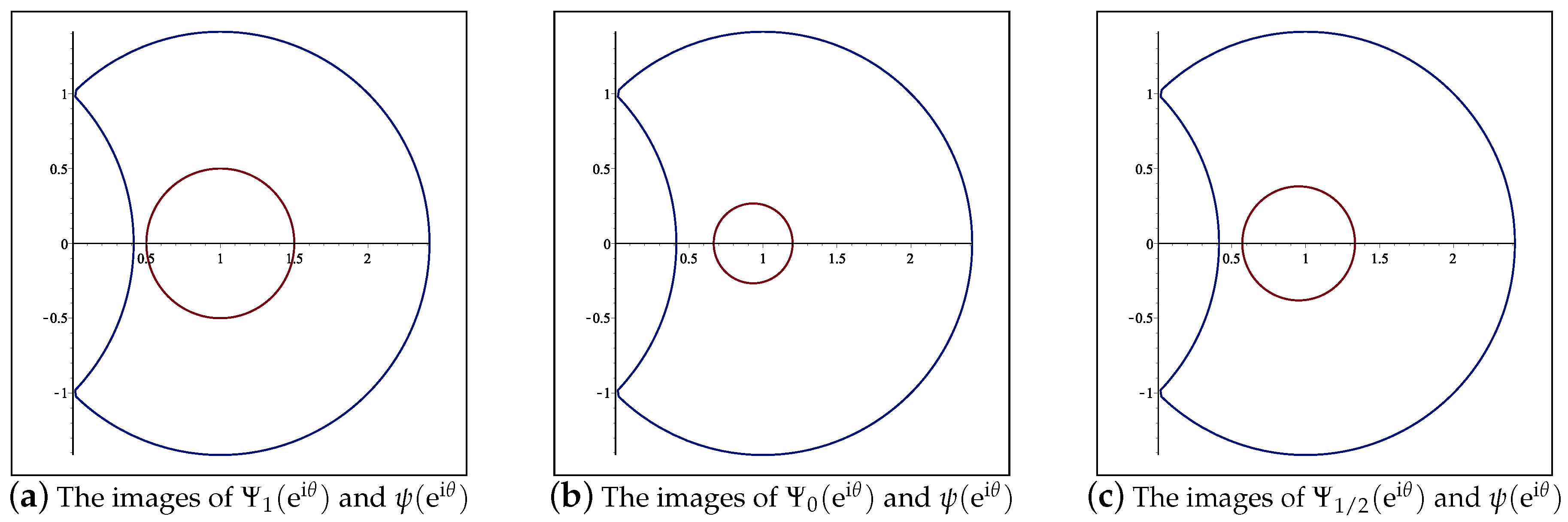
Remark 2. If we define the function by , , a simple computation yields to Considering the circular transformation with , and assuming that , we obtain that maps the unit disc onto the open disc that is symmetric respecting the real axes connecting the points and .
If , then , and for , , and , using the MAPLE™ software we get the next images of by like in the Figure 2: These show that , which is for some values of that is , whenever , for , , and . It follows that there exist values of the parameters , , and , such that .
Now, by suitably specializing the parameter , we define the new subclasses of as remarked below:
Remark 3. (i) For , let denote the subclass of , the members of which are given by (1) and satisfy the subordination condition (ii) For , let denote the subclass of , members of which are of the form (1) and if it satisfy the condition (iii) For the special case for , let , members of which are given by (1) and satisfy the subordination In the all of the above subordinations, and throughout the whole paper, the branch of the square root is chosen at the principal one, which is , and , .
Using the techniques of Libera and Zlotkiewicz [
11] and Koepf [
17], combined with the help of MAPLE™ software, we find Fekete–Szegő inequality and Hankel determinant for the function of the class
.
3. Coefficient Bounds and Fekete–Szegő Inequality
In our first result, we will determine coefficient bounds for , and this tends to solve the Fekete–Szegő problem for the subclass .
Theorem 1. If and is of the form (1), then Proof. If
, from (
6), it follows that there exists a function
with
and
,
, such that
Define the function
by
which is
and, since
with
and
,
, it follows that
.
Substituting the function
w from (
14) on the right-hand side of (
13) and simplifying, we get
and, by using (
4), the left-hand side of (
13) will be
where
,
, is given by (
5).
Hence, replacing (
15) and (
16) in (
13) and comparing the coefficients of
z,
and
, we get
Thus, from Lemma 1, we have
and, according to Lemma 2, it follows that
and
Replacing the values of
and
given by the relations (
11) and (
12) in (
20), respectively, and, denoting
, we get
for some complex numbers
x and
z, with
and
. Using the triangle’s inequality and substituting
, we get
Now, we will find the maximum of the function
on the closed rectangle
. Denoting
and using the MAPLE™ software for the following code
[> H :=(3*l^2-l+4)*p^3/(8*(1+l)*(2+l))-
(2*l^2+l-3)*(-p^2+4)*p*y/(2*(1+l)*(2+l))
- 1/4*(-p^2+4)*p*y+1/2*(-p^2+4)*(-y^2+1);
[> maximize(H, p=0 .. 2, y=0 .. 1, location);
we get
max(2, (3*l^2-l+4)/((1+l)*(2+l))),
{[{p=2}, (3*l^2-l+4)/((1+l)*(2+l))],
[{p=0, y=0}, 2]}
A simple computation shows that
whenever
; therefore,
which implies that
and the proof of our theorem is complete. □
Theorem 2. If is of the form (1), then, for any , we have Proof. If
is of the form (
1), from (
17) and (18), we get
where
Taking the modules for the both sides of the above relation, with the aid of the inequality (
7) of Lemma 2, we easily get the required estimate. □
For , the above theorem reduces to the following special case:
Corollary 1. If is given by (1) then, for any , we have Remark 4. If is given by (1) then, for the special case , we get If we take in Theorem 2, we get the next special case:
Theorem 3. 1. If the function is given by (1), and , then 2. Furthermore, if , then These results are sharp.
Proof. If
is given by (
1), from (
17) and (18), we get
where
From the assumptions, using the second above equality, it follows that
. We have
is equivalent to , and is equivalent to .
Then, taking the modules for both sides of the above equality, with the aid of the inequality (
8) of Lemma 3, we obtain the first estimates of Theorem 3.
For the proof of the second part, first we see that
is equivalent to
. Using the relations (
23) and (
17), and then applying the inequality (
9) of Lemma 3, we get
which represents the required inequality (
21).
Furthermore, we easily check that
is equivalent to
. From the relations (
23) and (
17), and then applying the inequality (
10) of Lemma 3, we obtain
which is the inequality (
21).
To prove that the bounds are sharp, we define the functions
and
,
, respectively, with
and
by
and
respectively. Clearly,
. In addition, we write
.
If or , then the equality holds if and only if f is or one of its rotations. When , then the equality holds if and only if f is or one of its rotations. If , then the equality holds if and only if f is or one of its rotations. If , then the equality holds if and only if f is or one of its rotations. □
4. Hankel Determinant Result for
The next result deals with an upper bound of for the subclass :
Theorem 4. If is given by (1) and Proof. If
, using a similar proof like in the proof of Theorem 1, from (
17), (
18), and (
19), we get
where
Using the relations (
11) and (
12) of Lemma 4, we get
with
,
, and
where
. Since
, it follows that
, hence we may assume without loss of generality that
, and, according to Lemma 1, it follows that
. Now, using the triangle’s inequality in (
26) and substituting
, we get
Next, we will find maximum of on the closed rectangle . Using the MAPLE™ software for the following code, where we denoted and ,
[>G :=abs(A)*p^4+abs(B)*(-p^2+4)*p^2*t+1/4*abs(C)*(-p^2+4)^2*t^2
+1/4*abs(D1)*p^2*(-p^2+4)*t^2+1/2*abs(E)*p*(-p^2+4)*(-t^2+1);
[> maximize(G, p=0 .. 2, t=0 .. 1, location);
max(16*abs(A), 4*abs(C)),
{[{p=2}, 16*abs(A)], [{p=0, t=1}, 4*abs(C)]}
or
max(16|A|, 4|C|), {[{p=2}, 16|A|], [{p=0, t=1}, 4|C|]},
We will prove that, under our assumption we have
, and therefore
Letting
and
, from (
24), it follows that
. A simple computation shows that
where
Since
then
if and only if the inequality
holds for all
. This last inequality is equivalent to
and a simple computation shows that
for all
. Therefore, the above inequality holds whenever the assumption (
24) is satisfied, hence
. Since
, we have
with
If , then , and using the inequality , we get . If , then , and, because , , it follows that .
Therefore, for all
, we have
. Since (
27) was proved, the upper bound of
on the closed rectangle
is attained at
and
, which implies the inequality (
25). □
Remark 5. By suitably specializing the parameter λ, one can deduce the above results for the subclasses of , and , which are defined, respectively, in Remark 3 (i) and (ii). Furthermore, by taking , we can easily state the result for the function class given in Remark 3 (iii). The details involved may be left as an exercise for the interested reader.


