Feature Keypoint-Based Image Compression Technique Using a Well-Posed Nonlinear Fourth-Order PDE-Based Model

Abstract

A digital image compression framework based on nonlinear partial differential equations (PDEs) is proposed in this research article. First, a feature keypoint-based sparsification algorithm is proposed for the image coding stage. The interest keypoints corresponding to various scale-invariant image feature descriptors, such as SIFT, SURF, MSER, ORB, and BRIEF, are extracted, and the points from their neighborhoods are then used as sparse pixels and coded using a lossless encoding scheme. An effective nonlinear fourth-order PDE-based scattered data interpolation is proposed for solving the decompression task. A rigorous mathematical investigation of the considered PDE model is also performed, with the well-posedness of this model being demonstrated. It is then solved numerically by applying a consistent finite difference method-based numerical approximation algorithm that is next successfully applied in the image compression and decompression experiments, which are also discussed in this work.

1. Introduction

The digital image compression represents an important image processing and analysis task whose purpose is to reduce the image file size without losing much information and while conserving its visual quality, so as to facilitate the image storing and transmission operations. The compression process, which could have an either lossless or lossy character, encodes the image content using fewer bits than its original representation [1].

The lossless compression algorithms remove or reduce considerably the statistical redundancy and recover exactly the image at decompression, without information loss. The following encoding algorithms are used for this type of compression: Huffman coding; aritmetic coding; run length encoding (RLE); LZW (Lempel–Ziv–Welch) encoding; or area coding, which is an enhanced 2D version of RLE [1,2,3]. Several well-known image formats, such as BMP, GIF, or PNG, are constructed using the lossless compression.

Lossy compression methods are characterized by higher compression rates, but they also lose an amount of image information. While the decompressed image versions are not identical to the originals, they look very similar. The lossy coding techniques include vector quantization, transformation-based encoding, fractal coding, block truncation coding, and sub-band coding [2,3]. Some very popular image standards based on lossy compression include JPEG, JPEG 2000, and other JPEG variants, which use transform-based coding (discrete cosine transform (DCT)- and discrete wavelet transform (DWT)-based image encoding) [1,2,3], and the MPEG standard with its versions [2,3].

The image compression techniques using partial differential equations (PDEs) represents a recently developed category of lossy compression methods. In the last years, PDEs have been increasingly applied in many static and video image processing and analysis fields, including image restoration [4], interpolation [5], segmentation [6], compression [7], registration [8], and optical flow estimation [9]. The PDE-based compression domain may also be considered as an application area of PDE-based inpainting (image reconstruction), because those compression algorithms use the PDE image interpolation schemes for decompression. The PDEs are rarely applied in the compression stage, usually being used by the pre-processing operations that prepare the image for the compression task. Thus, various coding techniques, such as random sparsification based coding, B-tree triangular coding (BTTC) [10], tree-based rectangular subdivision-based encoding [11], edge-based image coding [3,12], and clustering-based quantization [13], can be applied for image compression.

Depending on the inpainting solutions used in the decompression stage, various PDE-based compression techniques have been developed in the last decades. They include linear homogeneous diffusion-based approaches using the harmonic [12,14,15], biharmonic [15], and triharmonic inpainting operators [16], which provide successful results for cartoon compression [14], and depth map compression [12]. Moroever, some effective compression solutions have been obtained using the absolute monotone Lipschitz extension (AMLE) inpainting model [1,16] and the nonlinear anisotropic diffusion-based interpolation schemes derived from Perona-Malik [17], Charbonnier [18], total variation (TV) [19], and robust anisotropic diffusion (RAD) models [20].

More performant PDE-based image compression frameworks are those based on edge-enhancing diffusion (EED). Such a compression solution is the BTTC-EED image encoder introduced by Galic, Weickert et al. in 2005 [21]. It uses an edge-enhancing diffusion-based interpolation and an adaptive B-tree triangular coding-based image sparsification [10]. The BTTC-EED compression method outperforms JPEG standard, when the two are compared at the same high compression rate, but it is outperformed by JPEG 2000 coder. An improved version of this encoder is Q64 + BTTC(L)-EED, proposed by Galic et al. in 2008 [22]. The most successful EED-based compression technique is the rectangular subdivision with edge-enhancing diffusion (R-EED) codec developed by Schmaltz et al. [11]. It clearly outperforms the BTTC-EED schemes and other PDE-based compression algorithms, as well as the JPEG codec. R-EED also outperforms JPEG 2000 for gray-level images, when compared at high compression ratios. An improved version of it, which was introduced by P. Pascal and J. Weickert in 2014 for color image compression [23], outperforms JPEG 2000 for color images as well, at high compression rates.

We conducted a high amount of research in the PDE-based image processing and analysis domains, and constructed numerous variational and differential models for image filtering [24], inpainting [25], segmentation [26], and compression [27]. A novel PDE-based image compression framework is considered here. A feature descriptor keypoint-based image sparsification, followed by a lossless RLE-inspired sparse pixel encoding process, is performed in the compression stage, which is described in the next section. While other compression techniques based on the scale-invariant descriptors, like SIFT, KAZE, and others, use their feature vectors [28,29,30], our novel method uses only the locations of their key points. As the number of these keypoints is not high, the proposed scheme has the advantage of producing high compression rates with still good decompression results.

The sparse pixel decoding and the inpainting of the decoded sparse image are performed in the decompression stage, which is described in the third section. The proposed nonlinear fourth-order PDE model for structure-based interpolation, representing the main contribution of this work, is presented in its second subsection. This inpainting algorithm provides the main advantage of the proposed method compared with many other PDE-based compression solutions, producing better interpolation on the same sparse image. A mathematical treatment concerning its well-posedness is performed on this model in the third subsection, with the existence of a unique variational solution being rigorously demonstrated. Another original contribution is the consistent finite difference-based numerical approximation scheme that converges to that weak solution is then described. Our image compression experiments and the comparisons with some well-known codecs are discussed in the fourth section, while the conclusions of this research are drawn in the final section of this article.

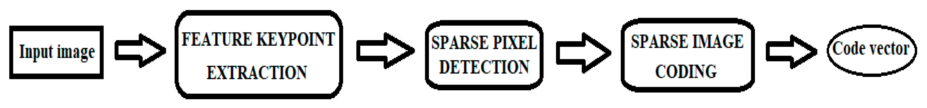
2. Interest Keypoint-Based Image Compression Algorithm

The compression component of the proposed framework consists of two main processes: image sparsification and sparse pixel coding. We could also add a pre-processing step that performs image enhancement using our past PDE-based filtering solutions [24]. The general scheme of the proposed compression algorithm is displayed in Figure 1.

So, first we propose a sparsification algorithm based on the interest keypoints of the image, which represent the keypoints of the most important scale-invariant image feature descriptors. Thus, we are interested only in the locations of these key points, as they represent locally high information contents, not in the feature vectors corresponding to those descriptors that are successfully used in many computer vision tasks such as image/video object detection, recognition, and tracking. This idea of using only these locations for the sparsification task is a rather new one in the image compression field. So, we perform a keypoint detection process for each of the following feature descriptors: SIFT, SURF, MSER, BRISK, ORB, FAST, KAZE, and Harris.

Scale Invariant Feature Transform (SIFT), introduced by David Lowe in 1999 [31], represents the most renowned local feature description algorithm. The SIFT keypoints are extracted as the maxima and minima values of the result of difference of Gaussians (DoG) filters applied at different scales on the image. Next, a dominant orientation is then assigned to each detected keypoint and a local feature descriptor is computed for it. The detected features are invariant to scaling, orientation, affine transforms, and illumination changes.

Speeded up Robust Features (SURF) is a fast image feature descriptor proposed by H. Bay et al. in 2008 [32]. The SURF keypoint detection is based on a Hessian matrix approximation. Thus, the determinant of the Hessian matrix is used as a measure of local change around the point and the keypoints are chosen where this determinant is maximal. The orientations of these keypoints are then determined and square regions are extracted, centered on these interest points, and aligned to their orientations. The distribution-based SURF descriptor is then modelled by summing Haar wavelet responses extracted for [4 × 4] sub-regions of the interest square region.

Maximally Stable Extremal Regions (MSER) were introduced by Matas et al. in 2002 [33]. They are defined by an extremal property of the intensity function within the region and on its outer boundary and are used as a blob detection technique. Each MSER is represented by a keypoint, which is the position of a local intensity minimum (or maximum), and a threshold that is related to the intensity function.

Features from Accelerated Segment Test (FAST) represents a well-known feature detection algorithn developed by E. Rosten and T. Drummond [34]. It is successfully used for corner detection and is also used to construct other image feature descriptors, such as BRISK and ORB. Binary Robust Invariant Scalable Keypoints (BRISK) is an effective rotation and scale-invariant fast keypoint detection, description and matching algorithm [35]. The keypoint detection is performed by creating a scale space, computing FAST score across scale space, performing a pixel level non-maximal suppression, computing sub-pixel maximum across patch, and the continuous maximum across scales. Then, the image coordinates are reinterpolated from scale space feature point detection. Then, a rotation and scale invariant feature descriptor is computed for each detected keypoint. Oriented FAST and rotated BRIEF (ORB) represents another fast robust local feature detector, introduced by E. Rublee et al. in 2011 [36]. It is based on a combination of the FAST descriptor and the visual descriptor BRIEF (Binary Robust Independent Elementary Features) [37].

KAZE represents a multiscale 2D feature detection and description algorithm in nonlinear scale spaces [38]. The KAZE features are detected and described in a nonlinear scale space by using the nonlinear diffusion-based filtering. Harris Corner detector [39], introduced by C. Harris and M. Stephens in 1988 as an improvement of the Moravec’s corner detector, is another well-known keypoint detection algorithm used by our sparsification approach.

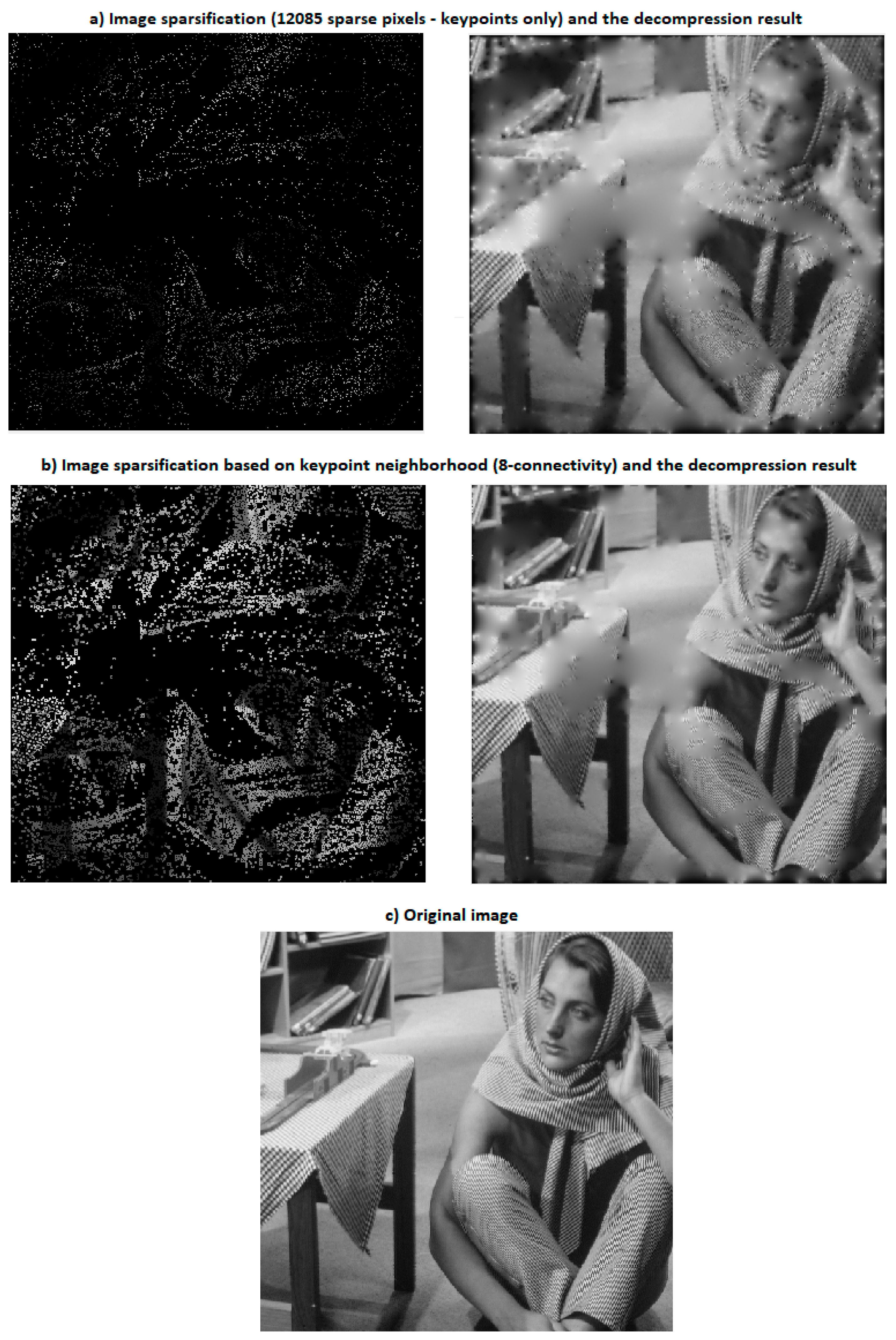
A keypoint detection example is described in Figure 2.

Our compression approach extracts all the SIFT, SURF, MSER, BRISK, ORB, FAST, KAZE, and Harris keypoints of the analyzed image, but, depending on their number, may not use all of them in the coding process. Depending on their content information, some images could have a high number of keypoints, while other may have only few interest points. Using a high number of keypoints in the sparsification process would produce a very good decompression result, but also a low compression rate, while using a low number of keypoints would lead to a weaker decompression output, but to a higher compression rate.

So, as we are interested in an optimal trade-off between the compression rate and the decompressed image quality, if the number of the detected keypoints exceeds a properly selected threshold depending on the image size (for example, a third of all pixels), the proposed algorithm may consider only the strongest k keypoints of each descriptor for the sparsifcation. Otherwise, all the detected keypoints can be used as sparse pixels, unless their numbers become lower than another threshold depending on image size. In this case, one uses the neighborhoods of the keypoints to add more sparse pixels.

Thus, a pixel neighborhood based on a four- or an eight-connectivity can be considered around each keypoint. While using four-neighborhood provides higher compression ratios, the eight-neighborhoods lead to better decompression result. Larger square $\left[n\times n\right]$ neighborhoods having the pixels corresponding to keypoints as centers could also be used to obtain more spare pixels and achieve better decompression results, but they would lead to lower compression rates, too. When the pixel neighborhoods are used, the pixels representing interest keypoints are not taken into account, with only the pixels around them being used as sparse pixels. Moreover, in order to improve the decompression output, a minimum density of keypoints could be set. Thus, we may apply a grid to the image, and if the number of keypoints in the given $\left[c\times c\right]$ cell of this grid (with $c\in \left(10,25\right)$) is lower than a certain threshold ((equal to 1, for example), then one or more keypoints should be randomly selected in that cell to be used as sparse pixels.

Then, the sparse image, which is identical to the original one in the sparse pixel’s locations and black (only pixels with 0 value) elsewhere, is obtained. A lossless RLE-inspired encoding is then performed on this image sparsification result [2].

So, the image is converted into a 1D vector, V, using the raster scan order, then a code C (V) is constructed for this vector. The proposed coding algorithm sets the current position in V at i = 1 and the code is initially a void vector C (V): = [ ]. At each iteration, the coding procedure determines the 3-uple $\left[V\left(i\right),n_i,n_i^0\right]$, where

$$V\left(i\right)=V\left(i+1\right)=\dots =V\left(i+n_i-1\right)$$

(1)

and

$$V\left(i+n_i\right)=\dots =V\left(i+n_i+n_i^0-1\right)=0$$

(2)

The 3-uple is then appended to the code vector as follows:

$$C(V):=\left[C(V),V\left(i\right),n_i,n_i^0\right]$$

(3)

and the current position becomes $i:=i+n_i+n_i^0$. When i becomes higher than the length of V, a final value, representing the ratio between the number of rows and the number of columns of the image, is added to C (V). The final code stored in this vector C (V) represents the image compression output. This lossless encoding algorithm may become a lossy coding scheme that improves the compression rates and ratios of (1) are replaced to $\Vert V\left(i+j\right)-V\left(i+j+1\right)\Vert \le low threshold,\forall j\in \left[0,n_i-2\right]$.

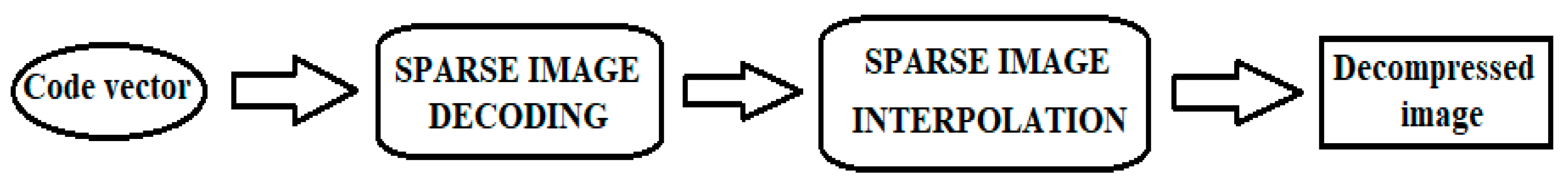
3. Nonlinear PDE-Based Image Decompression Technique

Two main operations are performed by the decompression component of the developed framework: the decoding process, followed by the reconstruction one. The general scheme of the decompression algorithm is displayed in Figure 3.

3.1. Image Decoding Scheme

Thus, a decoding algorithm is applied to the values encoded and stored by CV = C (V) computed by (3) to recover the vector V, which is initialized now as V: = [ ]. So, the code vector CV is processed iteratively and at each iteration i (starting with i = 1), a decoded sequence is added to the evolving vector as follows

$$V:=\left[V,\left(\underset{CV \left(i+1\right) \mathrm{times}}{\underbrace{CV\left(i\right),\dots ,CV\left(i\right)}},\underset{CV \left(i+2\right) \mathrm{times}}{\underbrace{\mathrm{0...0}}}\right)\right]$$

(4)

and the next current position in the code vector becomes $i:=i+3$.

This iterative decoding procedure continues while the value of i is lower than the length of CV. When i becomes equal to the length of the code vector CV, the obtained 1D vector V of length l(V) is transformed into a $\left[l(V)\sqrt{\frac{l(V)}{CV(i)}}\times \sqrt{\frac{l(V)}{CV(i)}}\right]$ matrix, which represents the decoded sparse image.

Then, this result of the decoding process is further processed by the reconstruction procedure of the decompression scheme. In the reconstruction step, the initial image is recovered, as well as possible, from the scattered data points of the sparse image, by performing a PDE-based interpolation process, which is described in the next subsection.

3.2. Novel Fourth-Order Partial Differential Equation-Based Inpainting Model

We propose a nonlinear fourth-order PDE-based scattered data point interpolation technique that performs effectively the image reconstruction process [5,25]. It is based on the following PDE inpainting model with boundary conditions:

$$\{\begin{array}{l}\frac{\partial u}{\partial t}-\alpha \psi \left(\left|{\nabla }^{2}u\right|\right)\nabla \cdot \left(\delta \left(\Vert {\nabla }^4{u}_{\sigma }\Vert \right)\nabla u\right)+\left(1-1_{\Gamma }\right)\left(u-u_0\right)=0,\mathrm{on} \left(0,T\right)\times \partial \Omega \\ u\left(0,x,y\right)=u_0\left(x,y\right),\hspace{1em}\forall \left(x,y\right)\in \Omega \\ u\left(t,x,y\right)=0,\hspace{1em}\mathrm{on}\left(0,T\right)\times \partial \Omega \\ \Delta u\left(t,x,y\right)=0,\hspace{1em}\mathrm{on} \left(0,T\right)\times \partial \Omega \end{array}$$

(5)

where $\alpha \in \left[1,2\right)$, $\Gamma \subset \Omega \subseteq R^2$ is the inpainting region that contains the black pixels of the sparse image represented here by the observed image $u_0:\Omega \backslash \Gamma \to R$ and $u_{\sigma }=u\ast G_{\sigma }$, where $G_{\sigma }\left(x,y\right)=\frac{1}{2\pi {\sigma }^2}{e}^{-\frac{x^2+y^2}{2{\sigma }^2}}$ is the 2D Gaussian filter kernel [1].

We construct a diffusivity function for this model, which is positive, monotonic decreasing, and converging to 0, such as to achieve a proper diffusion process. It has the following form:

$$\delta :\left[0,\infty \right)\to \left[0,\infty \right),\delta \left(s\right)=\gamma {\left(\frac{\eta (t,x,y)}{\left|\lambda \ln \eta (t,x,y)+\beta s^k\right|}\right)}^{\frac{1}{k+1}}$$

(6)

where the coefficients are $\lambda ,\gamma \in \left(0,1\right),\beta \in \left(1,3\right],k\ge 1$ and the conductance parameter $\eta (t,x,y)$ is a function depending on the coordinates and statistics of the evolving image and is computed by an algorithm that will be described later [24]. The Bi-Laplacian is used in the $\delta (\Vert {\nabla }^4{u}_{\sigma }\Vert )$ component to overcome more effectively the staircase effect.

The other positive function used within this partial differential equation-based model has the following form:

$$\psi :\left[0,\infty \right)\to \left[0,\infty \right), \psi \left(s\right)=\frac{{(\xi s^r+\nu )}^{\frac{1}{r+1}}}{\zeta }$$

(7)

where its coefficients are $\xi ,\nu ,\zeta \in \left[1,3\right)$ and $r\in \left(0,1\right)$. The term $\psi \left(\left|{\nabla }^{2}u\right|\right)$ is introduced to control the speed of the diffusion process and enhance the edges and other details.

The Dirichlet boundary conditions in (5) were chosen such that the proposed PDE model is well-posed. This fourth-order PDE-based interpolation scheme given by (5) reconstructs properly the observed image that is known only in a few locations, representing the sparse pixels. It performs the scattered pixel interpolation by directing the smoothing process toward the inpainting region and reducing it outside of that zone, using the inpainting mask given by the characteristic function $1_{\Gamma }\left(x,y\right)$ [5].

Thus, the reconstructed image would represent the solution of this nonlinear PDE model. So, the existence and unicity of such a solution is investigated in the following subsection, where the well-posedness of the proposed differential model is rigorously treated.

3.3. Mathematical Investigation of the Proposed PDE Model’s Validity

In this subsection, one investigates the mathematical validity of the nonlinear fourth-order PDE-based model introduced in the previous subsection. Thus, a rigorous mathematical treatment is performed on the well-posedness of the proposed PDE inpainting model (5) to demonstrate the existence and unicity of a variational (weak) solution for it [4,40,41].

It is convenient to transform (5) into a parabolic equation of porous media type. So, we obtain the following PDE model:

$$\{\begin{array}{l}{v}_t-\alpha \Delta \psi \left(\left|v\right|\right)\nabla \cdot \left(\delta \left(\Vert G_1\ast v\Vert \right)\cdot \nabla \left({\Delta }^{-1}v\right)\right)+\Delta \left(1-1_{\Gamma }\right)\left({\Delta }^{-1}v-u_0\right)=0,\mathrm{on} \left(0,T\right)\times \partial \Omega \\ v\left(0,x,y\right)=\Delta u_0\left(x,y\right),\hspace{1em}\left(x,y\right)\in \Omega \\ v\left(t,x,y\right)=0,\hspace{1em}\mathrm{on} \left(0,T\right)\times \partial \Omega \end{array}$$

(8)

where $G_1={\nabla }^2{G}_{\sigma }$ and $v={\nabla }^{2}u=\Delta u$.

We note that $\nabla \cdot \left(\delta \left(\Vert G_1\ast v\Vert \right)\nabla \left({\Delta }^{-1}v\right)\right)={\delta }_s\left(\Vert G_1\ast v\Vert \right)\left(\nabla G_1\ast v\right)\cdot \nabla \left({\Delta }^{-1}v\right)+\delta \left(\Vert G_1\ast v\Vert \right)v+\nabla \cdot \delta \left(\Vert G_1\ast v\Vert \right)$ and so (8) can be re-written as follows:

$$\{\begin{array}{l}{v}_t-\alpha \Delta \varphi \left(x,y,v\right)+\Delta \left(\left(1-1_{\Gamma }\right)\left({\Delta }^{-1}v-u_0\right)\right)=0,\mathrm{on} \left(0,T\right)\times \partial \Omega \\ v\left(0,x,y\right)=v_0\left(x,y\right)=\Delta v_0\left(x,y\right),\hspace{1em}\left(x,y\right)\in \Omega \\ v\left(t,x,y\right)=0,\hspace{1em}\left(x,y\right)\in \Omega ,t\in \left(0,T\right)\end{array}$$

(9)

where

$$\varphi \left(x,y,v\right)=\psi \left(\left|v\right|\right){\delta }_s\left(\Vert G_1\ast v\Vert \right)\left(\nabla G_1\ast v\right)\cdot \nabla \left({\Delta }^{-1}v\right)+\alpha \delta \left(\Vert G_1\ast v\Vert \right)v+\alpha \nabla \cdot \delta \left(\Vert G_1\ast v\Vert \right)$$

(10)

Therefore, instead of (1), we shall study the existence problem for the nonlinear parabolic problem (9). The following hypotheses are easily verified [40,41]:

• $\psi :\left[0,\infty \right)\to \left[0,\infty \right)$ is of class $C^1$ and ${\beta }_1\le \psi ’\left(r\right)\le {\beta }_2,\forall r\in R^{+}$ where ${\beta }_1,{\beta }_2>0$
• $\delta \in C^1\left(\Omega \times R\right),\delta >\rho >0$, where $\rho$ is a constant

By weak solution to problem (9), we mean a function $v:\left[0,T\right]\times \Omega \to R$, such that

$$v\in L^2\left(0,T;L^2(\Omega )\right)\cap C\left(\left[0,T\right];H^{-1}(\Omega )\right),v_t\in L^2\left(0,T;{\left(L^2\right)}^{*}\right)$$

(11)

where ${\left(L^2\right)}^{*}$ is the dual space of $L^2(\Omega )$ with the pivotal space $H^{-1}(\Omega )$, which is the dual space of the Sobolev space $H_0^1(\Omega )$, and

$$\begin{array}{l}{\displaystyle \underset{\Omega }{\int }{v}_t\left(t,x,y\right){\left(-\Delta \right)}^{-1}\phi \left(x,y\right)dxdy=\alpha }{\displaystyle \underset{\Omega }{\int }\varphi \left(x,y,v\left(t,x,y\right)\right)\phi \left(x,y\right)dxdy}\\ -{\displaystyle \underset{\Omega }{\int }\left(1-1_{\Gamma }\right)\left({\Delta }^{-1}v\left(t,x,y\right)-u_0\left(x,y\right)\right)\phi \left(x,y\right)dxdy}=0\end{array}$$

(12)

for all $\phi \in L^2(\Omega )$ [40,41].

We note, from (11) and (12), it follows that $\varphi \left(\cdot ,v\right)\in L^2\left(0,T;H_0^1(\Omega )\right)$, which implies v = 0 on $\partial \Omega$.

Theorem 1. 

Assume that$v_0=\Delta u_0\in L^2(\Omega )$and$v_0\ge 0$. Then, under the hypotheses (i) and (ii), and for sufficiently small T, there exists at least one weak solution$v\in C\left(\left[0,T\right];H^{-1}(\Omega )\right)\cap L^2\left(\left[0,T\right];H_0^1(\Omega )\right),v\ge 0$to Equation (9).

Proof. 

We consider the following set:

$\aleph =\left\{v\in C\left(\left[0,T\right];H^{-1}(\Omega )\right);{\Vert v\left(t\right)\Vert }_{H^{-1}(\Omega )}\le M,{\displaystyle \underset{0}{\overset{T}{\int }}{\displaystyle \underset{\Omega }{\int }{\left|v\left(t,x,y\right)\right|}^{2}dtdxdy\le M, }}v\ge 0 on\left(0,T\right)\times \Omega \right\}$ For each $w\in \aleph$, consider the following equation:

$$\{\begin{array}{l}{v}_t-\alpha \Delta \left(\psi \left(v\right)\varsigma +\delta \left(\Vert G_1\ast v\Vert \right)v+\nabla \cdot \delta \left(\Vert G_1\ast v\Vert \right)\right)+\Delta \left(1-1_{\Gamma }\right)\left({\Delta }^{-1}v-u_0\right)=0\\ v\left(0,x,y\right)=v_0\left(x,y\right)=\Delta u_0\left(x,y\right)\\ v\left(t,x,y\right)=0 \mathrm{on} \left(0,T\right)\times \partial \Omega \end{array}$$

(13)

where $\varsigma =\nabla \cdot \left({\delta }_s\left(\Vert G_1\ast v\Vert \right)\nabla \left({\Delta }^{-1}w\right)\right)$. For each $w\in \aleph$, the operator $A\left(t\right):L(\Omega )\to {\left(L^2\right)}^{*}$ defined by ${}_{{\left(L^2\right)}^{*}}\left(A\left(t\right)v,\phi \right)_{L^2(\Omega )}=\alpha {\displaystyle \underset{\Omega }{\int }\psi \left(v\right)}\varsigma \phi dxdy-{\displaystyle \underset{\Omega }{\int }\left(1-1_{\Gamma }\right)\left({\Delta }^{-1}v-u_0\right)}\phi dxdy+\alpha {\displaystyle \underset{\Omega }{\int }\left(\delta \left(\Vert G_1\ast v\Vert \right)v+\nabla \cdot \delta \left(\Vert G_1\ast v\Vert \right)\right)}\phi dxdy$ for $\forall \phi \in L^2(\Omega )$ is monotone, continuous, and coercive, that is, ${}_{{\left(L^2\right)}^{*}}\left(A\left(t\right)v,\phi \right)_{L^2(\Omega )}=C_1{\Vert \phi \Vert }_{L^2(\Omega )}^2-C_2{\Vert \phi \Vert }_{{\left(L^2\right)}^{*}}^2$.

Then, by Theorem 1.2., Chapter 2 in [41], it follows that Equation (13), that is,

$$\{\begin{array}{l}\frac{\partial v}{\partial t}+A\left(t\right)v=0,t\in \left(0,T\right)\\ v\left(0,x,y\right)=v_0\left(x,y\right)\end{array}$$

(14)

has a unique solution $v=F \left(w\right)$, $v\in L^2\left(0,T;L^2(\Omega )\right)$, $\frac{\partial v}{\partial t}\in L^2\left(0,T;{\left(L_2\right)}^{*}\right)$. We are going to show that F has a fixed point $w=F\left(w\right)$. If multiply the Equation (13) by $v$ and integrate it on $\left(0,t\right)\times \Omega$, we get the estimate for each $w\in \aleph$:

$${}_{{\left(L^2\right)}^{*}}\left(A\left(t\right)v,v\right)_{L^2(\Omega )}\ge \phi {\Vert v\Vert }_{L^2(\Omega )}^2-C$$

(15)

where the constant C > 0 and, therefore, we get

$${\Vert v\left(t\right)\Vert }_{H^{-1}(\Omega )}^2+s{\displaystyle \underset{0}{\overset{t}{\int }}{{\displaystyle \underset{\Omega }{\int }\left|v\left(s,x,y\right)\right|}}^{2}dsdxdy}\le C\left(M+1\right)T$$

(16)

Hence, for sufficiently small T and suitable M chosen, we have $F\left(w\right)\in \aleph ,\forall w\in \aleph$. Moreover, $F$ is continuous from $L^2\left(0,T;H^{-1}(\Omega )\right)$ to itself and, as easily seen, $F(\aleph )$ is compact in $L^2\left(0,T;H^{-1}(\Omega )\right)$, because by (13), we see that ${\Vert \frac{dv}{dt}\Vert }_{L^2\left(0,T;{\left(L^2\right)}^{*}\right)}\le C,\forall w\in \aleph$. Then, by the classical Schauder’s fixed point theorem [41], because $F(\aleph )\subset \aleph$, where $\aleph$ is a bounded convex set of $v\in L^2\left(0,T;H^{-1}(\Omega )\right)$ and $F(\aleph )$ is compact, there is $w*\in \aleph$ such that $F\left(w*\right)=w*$. Clearly, $u=w*$ is a solution to (8) as claimed. By Theorem 1, it follows a corresponding existence result for (5) via the transformation $u={\Delta }^{-1}v$; therefore, the proposed PDE model is well-posed. □

3.4. Finite Difference-Based Numerical Approximation Scheme

The unique weak solution of the proposed PDE-based inpainting model, whose existence has been demonstrated in 3.3, is determined by solving numerically the model given by (5)–(7). So, a consistent numerical approximation scheme is developed for this well-posed PDE model by applying the finite difference method [42].

We consider a grid of space size h and time step $\Delta t$ for this purpose. The space coordinates are quantized as $x=ih,y=jh,i\in \left\{1,\dots ,I\right\},j\in \left\{1,\dots ,J\right\}$, while the time coordinate is quantized as $t=n\Delta t,n\in \left\{0,\dots ,N\right\}$, where the support image has the size of $[Ih\times Jh]$.

The nonlinear partial differential equation in (1) is discretized using finite differences [4,39]. It can be re-written as follows:

$$\frac{\partial u}{\partial t}+\left(1-1_{\Gamma }\right)\left(u-u_0\right)=\alpha \psi \left(\left|{\nabla }^{2}u\right|\right)\nabla \cdot \left(\delta \left(\Vert {\nabla }^4{u}_{\sigma }\Vert \right)\nabla u\right)$$

(17)

Its left term is then approximated numerically using forward difference for the time derivative [42]. We get the next discretization for it, $\frac{u_{i,j}^{n+\Delta t}-u_{i,j}^n}{\Delta t}+\lambda \left(1-1_{\Gamma }\right)\left(u_{i,j}^n-u_{i,j}^0\right)$. Then, the right term is approximated using the discrete Laplacian and the discretization of the divergence component. First, one computes

$${\psi }_{i,j}=\psi \left(\Vert \Delta u_{i,j}^n\Vert \right)=\psi \left(\frac{u_{i+h,j}^n+u_{i-h,j}^n+u_{i,j+h}^n+u_{i,j-h}^n-4u_{i,j}^n}{h^2}\right)$$

(18)

The divergence component can be re-written as

$$\nabla \cdot \left(\delta \left(\Vert {\nabla }^4{u}_{\sigma }\Vert \right)\nabla u\right)=div\left(\delta \left(\left|\Delta \left(\Delta u_{\sigma }\right)\right|\right)\nabla u\right)=\frac{\partial }{\partial x}\left(\delta \left(\left|\Delta \left(\Delta u_{\sigma }\right)\right|\right)u_x\right)+\frac{\partial }{\partial y}\left(\delta \left(\left|\Delta \left(\Delta u_{\sigma }\right)\right|\right)u_y\right)$$

(19)

and is discretized as ${\delta }_{i+\frac{h}{2},j}\left(u_{i+h,j}^n-u_{i,j}^n\right)-{\delta }_{i-\frac{h}{2},j}\left(u_{i,j}^n-u_{i-h,j}^n\right)+{\delta }_{i,j+\frac{h}{2}}\left(u_{i,j+h}^n-u_{i,j}^n\right)-{\delta }_{i,j-\frac{h}{2}}\left(u_{i,j}^n-u_{i,j-h}^n\right)$, where

$${\delta }_{i\pm \frac{h}{2},j}=\frac{{\delta }_{i\pm h,j}+{\delta }_{i,j}}{2},{\delta }_{i,j\pm \frac{h}{2}}=\frac{{\delta }_{i,j\pm h}+{\delta }_{i,j}}{2}$$

(20)

$${\delta }_{i,j}=\delta \left(\Vert \Delta {\left(\Delta u_{\sigma }\right)}_{i,j}^n\Vert \right)=\delta \left(\frac{\Delta {\left(u_{\sigma }\right)}_{i+h,j}^n+\Delta {\left(u_{\sigma }\right)}_{i-h,j}^n+\Delta {\left(u_{\sigma }\right)}_{i,j+h}^n+\Delta {\left(u_{\sigma }\right)}_{i,j-h}^n-4\Delta {\left(u_{\sigma }\right)}_{i,j}^n}{h^2}\right)$$

(21)

where $\Delta {\left(u_{\sigma }\right)}_{i,j}^n=\frac{{\left(u_{\sigma }\right)}_{i+h,j}^n+{\left(u_{\sigma }\right)}_{i-h,j}^n+{\left(u_{\sigma }\right)}_{i,j+h}^n+{\left(u_{\sigma }\right)}_{i,j-h}^n-4{\left(u_{\sigma }\right)}_{i,j}^n}{h^2}$. From (6), we have

$${\delta }_{i,j}=\gamma {\left(\frac{\eta (n,i,j)}{\left|\lambda \ln \eta (n,i,j)+\beta {\Vert \Delta {\left(\Delta u_{\sigma }\right)}_{i,j}^n\Vert }^k\right|}\right)}^{\frac{1}{k+1}}$$

(22)

where the conductance parameter is determined as follows:

$$\delta \left(i,j,n\right)=\left|\mu \left(\Vert \nabla {\left(u_{\sigma }\right)}_{i,j}^{n-1}\Vert \right)+\kappa n\right|$$

(23)

where $\kappa \in \left(0,1\right]$.

Therefore, we get the following numerical approximation:

$$\begin{array}{l}\frac{u_{i,j}^{n+\Delta t}-u_{i,j}^n}{\Delta t}+\lambda \left(1-1_{\Gamma }\right)\left(u_{i,j}^n-u_{i,j}^0\right)=\alpha {\psi }_{i,j}\\ \left[{\delta }_{i+\frac{h}{2},j}\left(u_{i+h,j}^n-u_{i,j}^n\right)-{\delta }_{i-\frac{h}{2},j}\left(u_{i,j}^n-u_{i-h,j}^n\right)+{\delta }_{i,j+\frac{h}{2}}\left(u_{i,j+h}^n-u_{i,j}^n\right)-{\delta }_{i,j-\frac{h}{2}}\left(u_{i,j}^n-u_{i,j-h}^n\right)\right]\end{array}$$

(24)

One may consider the parameter values $\Delta t=h=1$. So, (24) leads to the next explicit iterative numerical approximation algorithm:

$$\begin{array}{l}{u}_{i,j}^{n+1}=u_{i,j}^n\left(\lambda \left(1_{\Gamma }-1\right)+1\right)+\lambda u_{i,j}^0+\\ \alpha {\psi }_{i,j}\left[{\delta }_{i+\frac{1}{2},j}\left(u_{i+1,j}^n-u_{i,j}^n\right)-{\delta }_{i-\frac{1}{2},j}\left(u_{i,j}^n-u_{i-1,j}^n\right)+{\delta }_{i,j+\frac{1}{2}}\left(u_{i,j+1}^n-u_{i,j}^n\right)-{\delta }_{i,j-\frac{1}{2}}\left(u_{i,j}^n-u_{i,j-1}^n\right)\right]\end{array}$$

(25)

The numerical approximation scheme (25) is applied to the evolving image u for n taking values from 0 to N. It is consistent to the nonlinear fourth-order PDE inpainting model (5) and converges to its variational solution representing the recovered image. The number of iterations required by a proper reconstruction is quite high (hundreds of steps), depending on the number of sparse pixels and the size of the observed image.

The final inpainting result, $u^{N+1}$, also represents the lossy image decompression output. The obtained decompressed image is not identical to the initial image, because of the loss of information produced by our PDE-based framework, but has a high visual similarity.

4. Experiments and Method Comparison

The nonlinear PDE-based compression framework proposed here was applied successfully on hundreds of digital images. Well-known image collections, such as the volumes of the USC-SIPI database and the Image Repository of University of Waterloo [43], were used in our simulations. These simulations were conducted on an Intel (R) Core (TM) i7-6700HQ CPU 2.60 GHz processor on 64 bits, operating Windows 10. The MATLAB environment was used for the software implementation of the described numerical interpolation algorithm.

It works properly for both clean and noisy images and achieves good values for the compression’s performance measures, such as the compression rate (in bits per pixel bpp), the compression ratio, and the fidelity or quality. The described technique could achieve higher compression ratios by modifying some coding-related operations (see the discussions in the second section about using larger sparse pixel neighborhoods, transforming (1) and further processing the code vector), but the fidelity or quality measure may be negatively affected in those cases and decrease.

The compression component of this framework has a low computational complexity, as both the image sparsification and the sparse pixel encoding algorithm are characterized by low complexities and short execution times, of several seconds. The sparse pixel decoding approach also has a very low complexity, but the entire decompression technique is characterized by a much higher computational complexity, because of its more complicated nonlinear fourth-order PDE-based sparse pixel interpolation algorithm that performs a lot of computations, and a longer running time.

The performance of our decompression technique was assessed by applying similarity measures such as the peak signal-to-noise ratio (PSNR), mean squared error (MSE), and structural similarity index (SSIM) [44]. The decompressed versions of the images encoded using the proposed approach achieve good values of these metrics when measured against their originals. The compression rates obtained from the performed experiments lie between 0.30 and 0.75 bpp, which corresponds to compression ratios from 20:1 down to 11:1.

Some examples of image compression processes performed using our framework are described in Figure 4.

Compression method comparison was also performed. We compared the proposed approach to other image compression techniques, some of them based on PDEs, by applying similarity measures [44], like PSNR, MSE, and SSIM, for them at the same compression rates.

The compression component of our framework, using a scale-invariant feature keypoint-based image sparsification and an effective sparse pixel encoding algorithm, outperforms the compression schemes using other scattered data point selection and coding methods, such as the random sparsification, the edge-based sparsification and coding, or even the BTTC, providing better compression rates. The proposed nonlinear fourth-order PDE-based decompression technique provides better results than other PDE inpainting models, achieving better PSNR and SSIM values, although it has some disadvantages of its own. Given the high complexity of the interpolation algorithm (25), which requires many processing steps, our decompression scheme does not execute very fast. It may need more than 1 min for large images. Moreover, given the structural character of the PDE-based inpainting model (5), the proposed framework does not properly decompress the image textures.

Thus, we compared our PDE-based interpolation algorithm to other well-known PDE inpainting models of various orders in the decompression stage, with the same sparsification solution being chosen for compression. So, image interpolation schemes based on biharmonic smoothing, TV inpainting, and the fourth-order You–Kaveh model [45] adapted for inpainting were considered. Keypoint-based, edge-based, and random sparsification solutions were used in the coding stage. The PDE inpainting model proposed here outperforms the other PDE-based schemes, providing better values of the performance metrics (average PSNR) in all these sparsification cases, as it results from

Table 1. Method comparison: the performance of several partial differential equation (PDE) inpainting models in decompression stage. TV, total variation.

Sparsification Technique	The Proposed PDE Scheme	Biharmonic Inpainting	TV Inpainting	Fourth-Order PDE Model
Keypoint-based sparsification (described here)	25.3475 (dB)	24.4917 (dB)	22.9432 (dB)	23.4215 (dB)
Edge-based sparsification	25.1853 (dB)	24.3421 (dB)	22.1975 (dB)	22.1484 (dB)
Random sparsification (8% pixels)	20.2316 (dB)	18.9323 (dB)	16.9824 (dB)	17.1544 (dB)

. It also results from the following table that our feature keypoint-based sparsification technique outperforms both the random keypoint selection and the edge-based sparsification schemes.

The obtained values of the similarity metrics illustrate the effectiveness of the nonlinear PDE-based compression method described here that outperforms some well-known compression algorithms. Thus, our framework provides better decompression results than image compression techniques using random sparsification, edge-based coding, or B-tree triangular coding with PDE inpainting models like those using harmonic, biharmonic, and triharmonic smoothing, AMLE inpainting, and the second-order anisotropic diffusion-based inpainting schemes. It also outperforms the BTTC-L compression [10] and performs slightly better than the BTTC-EED model and the JPEG standard, at higher compression rates, while it is outperformed by the JPEG 2000 codec and the R-EED compression.

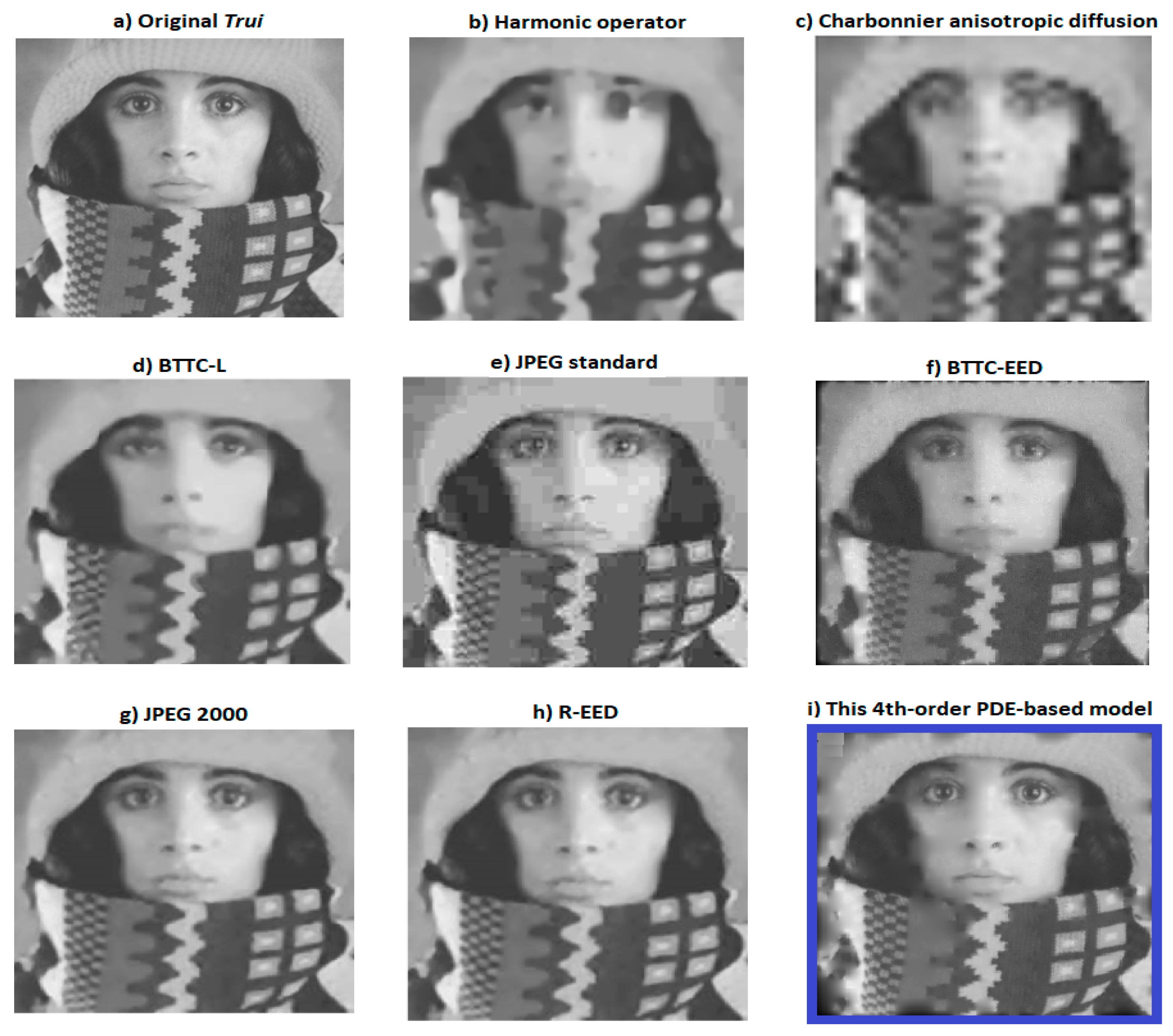
Several other method comparison results are displayed in Figure 5 and

Table 2. Average peak signal-to-noise ratio (PSNR) and structural similarity index (SSIM) values obtained by various methods at 0.4 bpp compression rate. BTCC, B-tree triangular coding; EED, edge-enhancing diffusion.

Compression Method	Average PSNR	Average SSIM
The proposed fourth-order PDE-based technique	26.3475 (dB)	0.6815
Harmonic inpainting-based compression	20.8495 (dB)	0.5167
Charbonnier diffusion-based model	22.3321 (dB)	0.5534
BTTC-L	23.1485 (dB)	0.6102
BTTC-EED	26.2378 (dB)	0.6723
JPEG	26.1075 (dB)	0.6546
JPEG 2000	26.8379 (dB)	0.7047
R-EED	27.1465 (dB)	0.7161

. Thus, the next figure contains the results obtained by some compression approaches on the [256 × 256] Trui image, at a compression rate of 0.40 bits/pixel.

The decompression output of the nonlinear PDE-based method proposed here is displayed in (i). The average PSNR and SSIM values obtained by the respective encoding approaches are displayed in Table 2. One can see that only JPEG 2000 and R-EED produce higher, but still comparable, metric values than the described compression technique.

5. Conclusions

A novel lossy image coding technique, which is based on the scale-invariant feature keypoint locations in the compression stage and a nonlinear fourth-order PDE-based model in the decompression stage, was proposed in this paper. The nonlinear partial differential equation-based model that was introduced, mathematically investigated, and numerically solved represents the major contribution of this work. In fact, it was the main purpose of this work to develop and analyze a new well-posed nonlinear partial differential equation-based interpolation model that can be successfully applied in the image compression domain. Beyond compression, however, the proposed PDE scheme can be successfully used for solving any inpainting task, like object or text removal, and an adapted version of it can be used efficiently in the image denoising and restoration domain.

While the PDE-based image decompression schemes are usually based on second-order diffusion equations, we proposed a more complex nonlinear fourth-order PDE inpainting model for the decompression task. Given the 2D Gaussian filter kernel involved in its componence, it performs efficiently in both clean and noisy conditions. Its well-posedness was rigorously demonstrated here and a consistent finite difference method-based approximation scheme was constructed to determine numerically the unique variational solution of it.

While the most important and original contributions of the developed framework are related to its decompression component, some novelties are brought in the compression stage, too. Thus, we proposed a novel image sparsification solution that is based only on the locations of the SIFT, SURF, MSER, BRISK, ORB, FAST, KAZE, and Harris keypoints and not on their features, and a sparse pixel encoding algorithm that is inspired by RLE. Although the proposed PDE-based inpainting algorithm may provide better decompression results when used in combination with some other sparsification models, this new keypoint-based image sparsification method has the advantage of using a rather low number of scattered data points and still leading to a good output.

The performed experiments and method comparisons illustrate the effectiveness of the proposed technique. It outperforms many existing image compression models and provides comparable good results with some state-of-the-art approaches. It has some drawbacks related to the running time, which can be quite long for large images, given the high computational complexity of the keypoint detection and sparse pixel encoding, decoding, and interpolation algorithms, and to the structural character of the PDE-based inpainting scheme, which also leads to weaker decompression results for the textured images. So, investigating some solutions to reduce the complexity of this technique, especially in the decompression stage, to get a lower execution time, and to improve the texture compression results, will represent the focus of our future research in this field.