Abstract
Predicting anomalous emission of pollutants into the atmosphere well in advance is crucial for industries emitting such elements, since it allows them to take corrective measures aimed to avoid such emissions and their consequences. In this work, we propose a functional location-scale model to predict in advance pollution episodes where two pollutants are involved. Functional generalized additive models (FGAMs) are used to estimate the means and variances of the model, as well as the correlation between both pollutants. The method not only forecasts the concentrations of both pollutants, it also estimates an uncertainty region where the concentrations of both pollutants should be located, given a specific level of uncertainty. The performance of the model was evaluated using real data of SO and NO emissions from a coal-fired power station, obtaining good results.
1. Introduction
Forecasting air quality and concentrations of pollutants in the atmosphere by means of statistical methods is an active area of research given the transcendence of the problem and the difficulty to find optimal solutions using deterministic mathematical models. Among the different methods that can be found in the literature to tackle this problem, models for time series analysis such as the integrated autoregressive moving average—ARIMA [1,2,3], multivariate regression [4,5,6,7], generalized linear or additive models (GAM) [8,9,10,11] and artificial neural networks (ANN) [12,13,14,15,16,17,18,19] are the most extended. Due to the increased access to continuous data over time, functional data analysis [20,21] was also proposed for air quality forecasting and outlier detection [22,23,24]. Parametric [25,26] and nonparametric [27,28,29] functional regression methods were tested. A functional framework allows considering the inherent correlation between observations, instead of considering them as independent realizations of an underlying stochastic process. Some functional approaches add related meteorological variables to the models [30,31,32,33,34], which can improve the result of the predictions and help to understand the process underlying the evolution of the pollutants.
Most of the documents in the literature propose solutions to predict the concentration of each pollutant individually, being much scarcer those focused on predicting more than one pollutant at a time. Vector autoregressive moving average (VARMA) [35,36] and vector autoregressive integrated moving average (VARIMA) [37] models were applied to reach this objective. In this work, we proposed a method for the simultaneous forecasting of pollution episodes when two pollutants, i.e., SO and NO, are involved. Apart from transport, one of the main sources of these pollutants is public electricity and heating. Their negative effects on human health are well known, and goes for mild (i.e., eyes irritated, nose or headache) to severe (i.e., lung damage or reduced oxygenation of tissues). They also have negative effects on animals and plants, as well as in other substances, such as water and soils. In addition, NO is a precursor of the tropospheric ozone. High levels of ozone contributes to climate change, cause adverse impacts on health and can damage vegetation.
Pollution episodes (incidents) are abnormally large emissions of one or more pollutants in short periods of time. Although the improvement of the chemical processes and particle filter systems have significantly reduced the amount and intensity of the pollution episodes, they are still of particular interest for the industries, as they may be subject to sanctions, or for other reasons, such as public health deterioration or industry discredit. Therefore, pollution industries, such as coal-fired power plants, are very interested in determining in advance when these episodes of excessive contamination might occur. Specifically, this is the purpose of our work: forecasting pollution episodes of SO and NO early enough to allow corrective measures to be taken. Our approach uses a location-scale model [11,38,39] that treats the predictors, the concentrations of both pollutants over time, as functions, while the response is a scalar, the concentration of the pollutants some time in advance. The novelty of our approach is the combination of a biviariate location-scale model with functional additive models. This method combines the simplicity of the location and scale models with the capacity of functional data analysis to deal with data in the form of functions.
The document is structured as follows: In Section 2 we show the mathematical model proposed to solve the problem under analysis and the algorithm used to estimate a solution from the data. Section 3 is devoted to test the validity of the model using real data. Finally, a discussion of the results and the main conclusions of our work are exposed in Section 4.
2. Methodology
2.1. Mathematical Model
Let be a set of observations of a stochastic process, , where , are predictor covariates and , with , a response variable. In this context, the following bivariate location-scale model [40,41] is assumed
where represents the Cholesky decomposition of the variance-covariance matrix
so that . To guarantee the model identification in (1), the bivariate residuals are assumed to be independent of the covariates, with zero mean, unit variance, and zero correlation. Despite we do not assume any distribution for the error term, within the framework of functional data analysis this work might be addressed under the assumption of other structures for error distribution: generalized Gauss-Laplace distribution that relax the constrictive assumption of the normal distribution errors [42], generalized linear mixed models (GLMMs) [38] to estimate random effects and dependent (temporal or spatial) errors, and generalized additive models for location, scale and shape (GAMLSS) [43] to model the dynamically variable distribution, considering skewness and kurtosis.
We define the unconditionally probabilistic region for the errors as
f being the density function of the bivariate residuals and k the quantile of . Then, for a given , we define a conditional - uncertainty region for containing of the observations as:
2.2. Estimation Algorithm
To implement an algorithm that allows applying the mathematical model exposed in the previous section, we propose using a functional additive models to estimate the means, variances and covariances in (1). Given a sample of size n, , where , the steps of the proposed estimation algorithm are the following:
Step 1: Perform a decomposition of each covariate in basis functions of the form , where () are K basis functions (i.e., B-splines, wavelets), and are either the coefficients of an expansion in fixed basis or the principal component scores of the Karhunen-Loève expansion [44,45]. As a result, we obtain the transformed covariates
Step 2: For , fit an additive model to the sample and obtain an estimation of the means
and then estimate from the sample as
Then, compute the correlation , which is related to the covariance by , using the sample , as follows:
being
where , and are smooth and unknown functions, , and are coefficients, p the number of predictors (covariates), and K the number of basis. Please note that the link functions and used in the variance and correlation structures, respectively, ensure that the restrictions on the parameter spaces ( and are maintained. Moreover, in order to guarantee the identification of the model, we assume that all the means of functions , and are zero.
Step 3: Compute the standardized residuals
where
with .
Step 4: Obtain the kernel estimation of the bivariate density given by
where is the kernel which is a symmetric probability density function and is a positive definite matrix. Then, obtain the unconditional bivariate uncertainty region on the residual scale as
being the empirical quantile of the values . Finally, for a given , the conditional bivariate uncertainty region is estimated according to (3)
3. Case Study: Joint Forecasting of Pollution Episodes
The mathematical model exposed in the previous section was applied to the forecasting of pollution episodes registered at a coal-fired power station located in the northwest of Spain. and are two of the main air pollutants generated by combustion processes, and both have harmful effects on human health. Moreover, it was proven that both pollutants are correlated [46], which is consistent with the model in (1). Fortunately, pollution episodes are not very frequent and the trend is that they will become scarcer as technology advances.
Let be the present time measured each five minutes, and and the concentrations obtained respectively by the series of bi-hourly SO and NO means at instant . Being the prediction horizon time, the interest is to predict
and provide an uncertainty region for these estimations given a specific value of , using the predictive covariates
where represents the first derivatives of the functions that approximate the concentrations of both pollutants. These derivatives are obtained from the functional representation of the discrete data, according to Step 1 of the estimation algorithm. Please note that represents the lagged time used in the predictors. In particular,, we are interested in predicting an hour in advance, according to the requirements of current Spanish legislation and, therefore, we will consider (60 min) from now on.
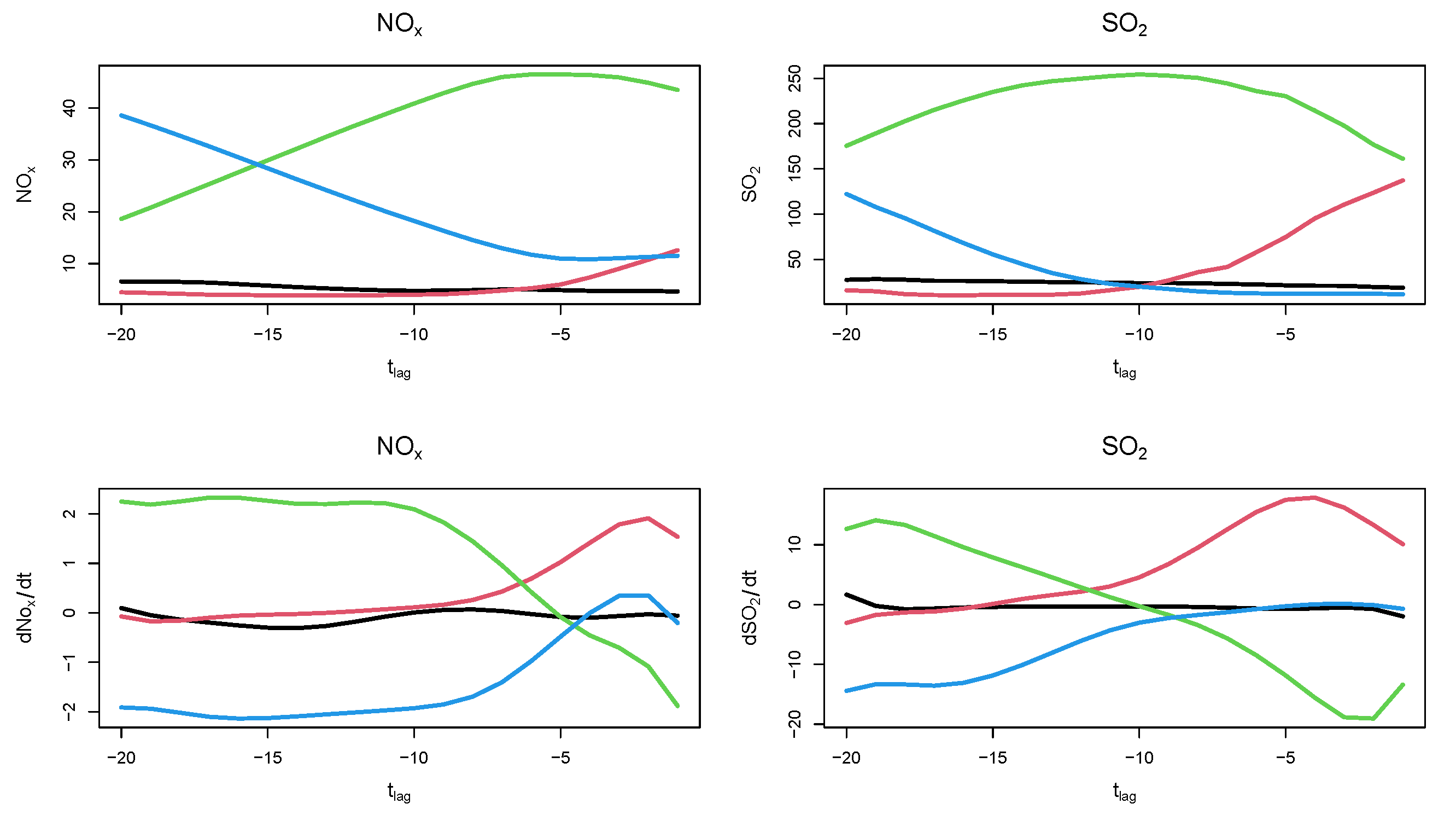
Most of the time, these concentrations times series are low, close to zero, and in order to obtain a reasonably large number of pollution incidents, we took as our sample a historical matrix with pollution data of approximately 12 years, which includes a considerable number of pollution episodes (see [9] for a detailed description of the historical matrix construction). In summary, in the historical matrix not all the data are used, but only part of them, following a quantile-weighted criterion. This means that the larger the concentration, the greater the number of observations of that concentration in the sample. Figure 1 shows a sample of the historical matrix, on top are the curves of both pollutants measured in discretization points and evaluated in 5 B-spline basis functions of order . On the bottom, the first derivative of the B-spline curves with order are represented.
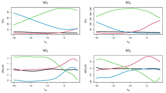
Figure 1.
Five curves of the historical matrix for pollutants ) and their corresponding first derivatives , observed in a period of time .
In this paper, we tested four models using as predictors different combinations of the covariates that include the concentrations of both pollutants and their first derivatives. In particular, we will consider models given by:
The four considered models, M, M, M and M, are configured in Table 1 where the cross X indicates the covariates included in each model.

Table 1.
Selected models from equation in (11). Cross X indicates the covariates included in each of the four considered models. The derivatives of the functions are indicated with a single quote.
To validate and compare the four proposed models, we randomly select from the full historical matrix a training set and a test set .
The estimates , , were obtained from the samples in the first matrix . The bivariate uncertainty regions for the values of the covariates on the second matrix were obtained using (3).
The estimated coverage is given by
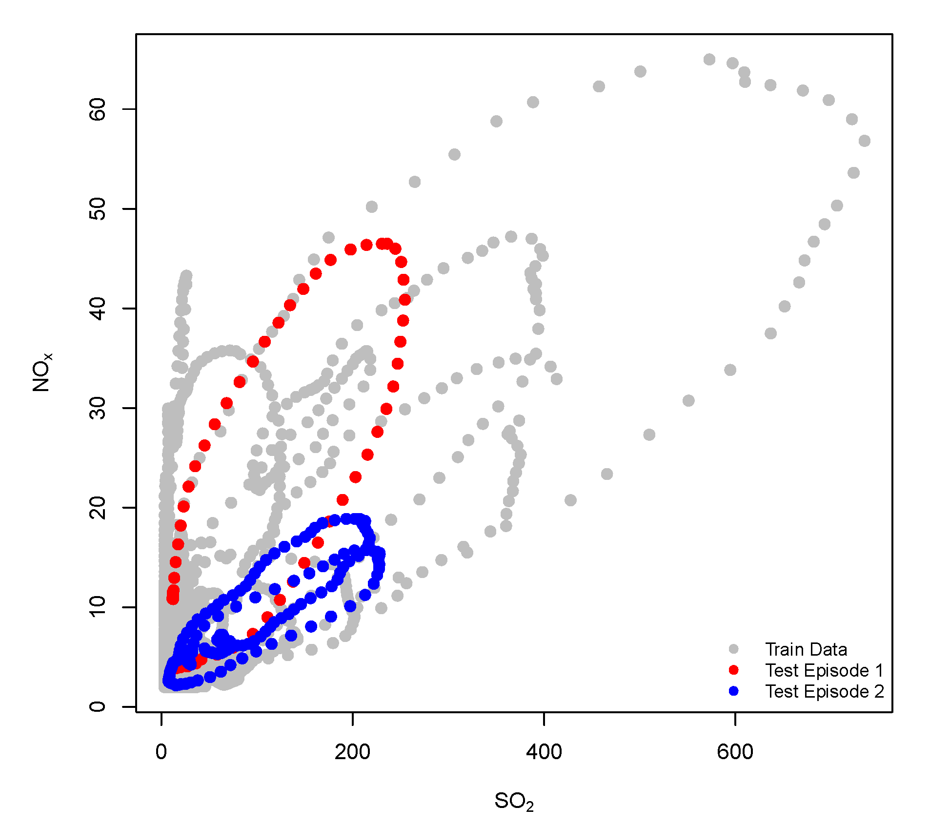
The performance of the proposed predictors was evaluated in two pollution incidents. A bivariate representation of these episodes is shown in Figure 2. The orientation of the points shows a clear correlation between both pollutants although the range of concentrations is quite different.

Figure 2.
Observed and forecasted concentrations of SO and NO for two pollution episodes.
The nominal and the estimated coverages for different time lags and training sample sizes are shown in Table 2. The coverages correspond to the bivariate solution, and were obtained for consecutive observations that might or might not correspond to pollution incidents.

Table 2.
Nominal and estimated coverages for each of the four models under study. Two time lags, , , two sizes of the training sample and , and two numbers of principal components, K = 3 and K = 5, were considered. Results correspond to the test sample.
RMSE values for each model are shown in Table 3, considering an expansion of the functions in three or five principal components, and lags and . Please note that this table makes reference to the marginal distributions, and that the range of concentrations for each pollutant is very different, therefore the RMSE values are also different.

Table 3.
RMSE values for two pollution episodes and the four models tested, considering curves with two different time lags, size of the training samples and number of principal components.
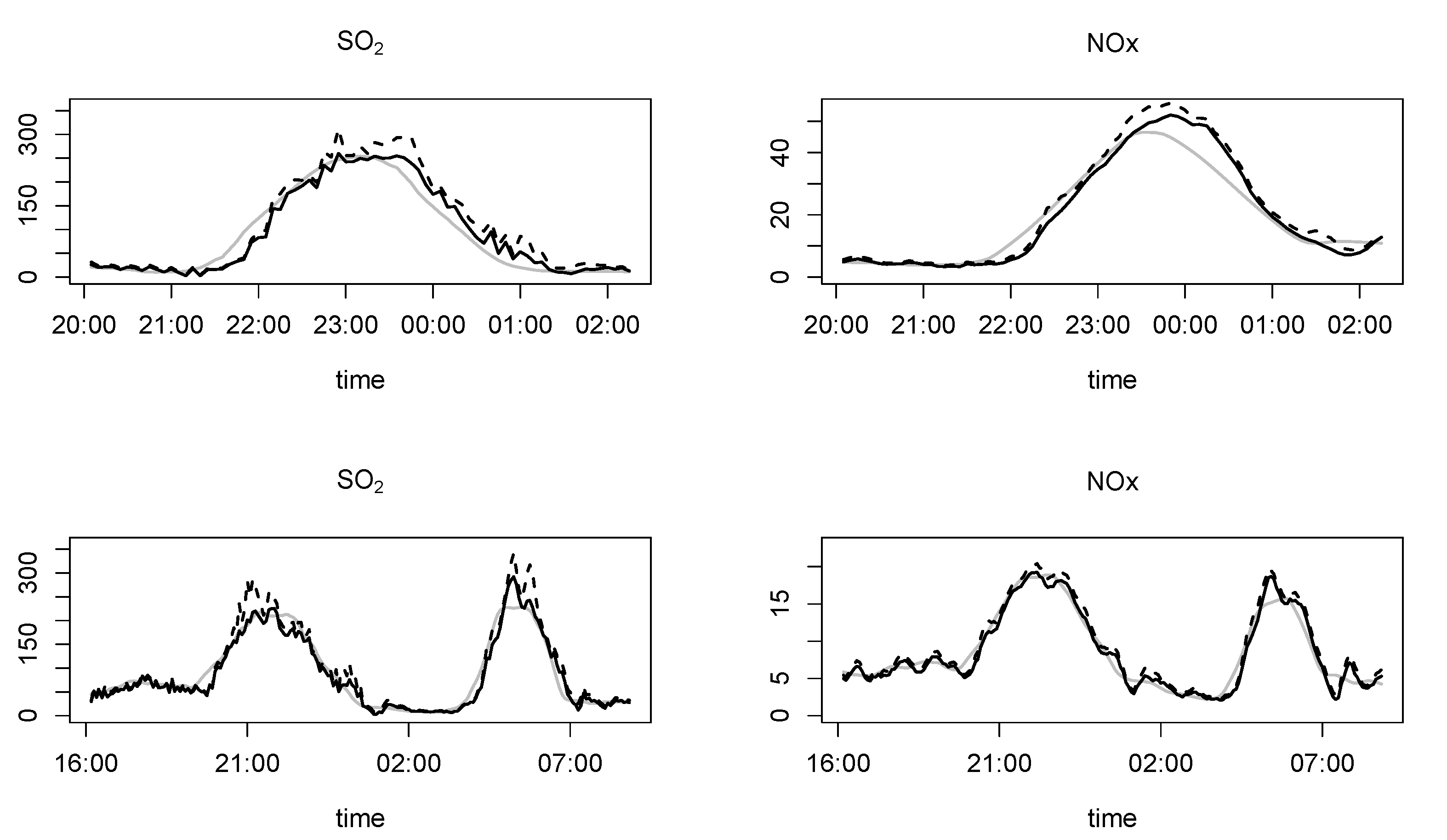
For the two episodes analyzed, Figure 3 shows the observed and the predicted values as well as the quantile for , calculated for the test sample. The results correspond to curves observed in ten points () and represented in a basis expansion in three functional principal components. These univariate confidence intervals were respectively constructed from (11) as and , and being the 0.95 quantile of the distributions of errors and , respectively.
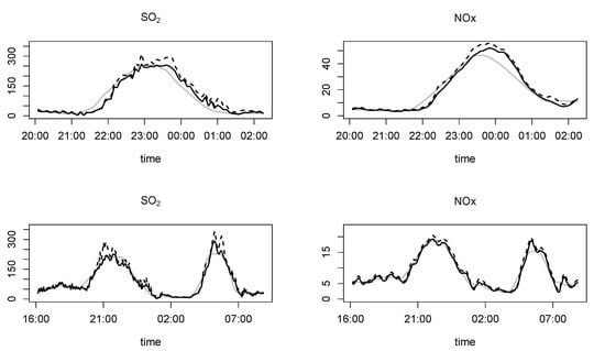
Figure 3.
Observations (solid black line), mean (solid gray line) and quantile estimations (discontinuous line) for both pollutants, SO and NO and for two pollution episodes.
Table 4 shows the maximum consumed memory and the runtime (in seconds) for the four models tested and two different dimensions of the submatrices are executed in a Intel Core i7-2600K with 16 GB of RAM.

Table 4.
Maximum memory consumption (MB) and computation time (seconds) for the four models tested, , following different strategies concerning the time lag, , the size of the training sample, , and the number of basis functions, K.
4. Discussion
We begin the discussion of the results analyzing Table 2 that show the estimated coverage for the bivariate prediction depending on the time lag, the size of the training sample, the number of principal components and the model used. It can be appreciated that the estimated coverages are generally lower than the theoretical coverages, although very close. Therefore, the mathematical models proposed show a good performance although there is a trend to underestimate the observed values. This effect can also be appreciated in Figure 3, where the mean tends to be under the observed values. Then, in order to be on the safe wide, it would be preferable to use the quantile , which provides greater guarantee of predicting the highest values of the pollution episodes. Regarding the rest of the parameters, it is not possible to establish a combination of them that provides the best results. However, in general they were obtained for the lowest training size, , and for models that includes one or two derivatives (models and ).
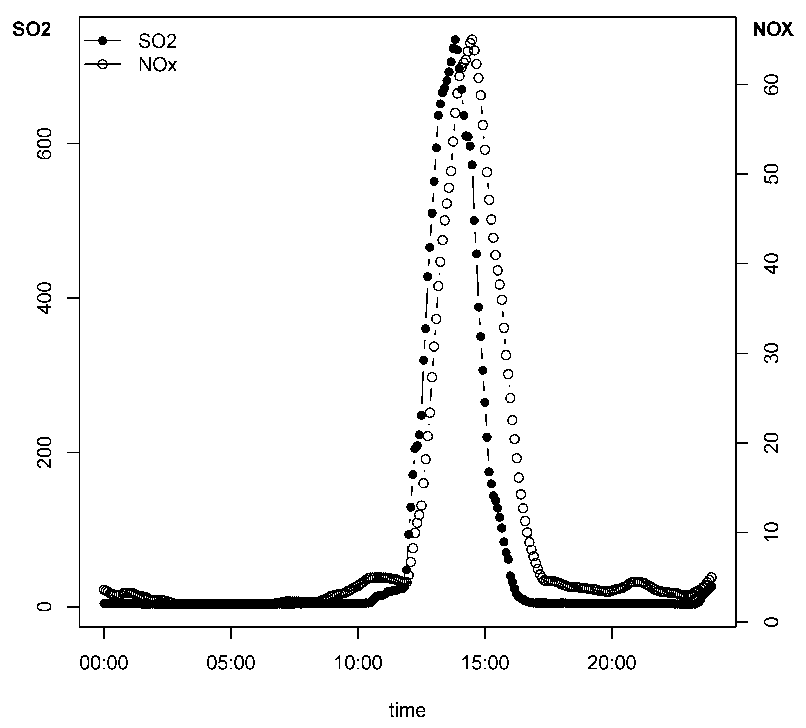
The prediction errors are shown in Table 1, where the best results (minimum RMSE) are marked in bold. As can be seen, they correspond to model for NO and model for SO. In both cases, these models incorporate the derivatives of the original functions. Accordingly, we conclude that the derivatives contribute positively to improve the results, which reinforces the role of the functional approach. However, there is an asymmetry between both pollutants: using the concentrations of SO and their derivatives improves the results for NO, but using the concentrations of NO and their derivatives is not an advantage in the estimation of SO. When SO and NO concentrations of both episodes are plotted against time (Figure 4), a slight advance can be seen on the first pollutant compared to the second, which would explain this asymmetry.

Figure 4.
Example of a pollution incident showing SO and NO concentrations versus time. Notice that there is an advance in the first pollutant compared to the second.
With respect to the time lag, the minimum RMSE values were obtained for the shorter period of time , so it seems that using 20 observations to predict one our in advance introduced noise into the model instead of adding useful information. This result is in agreement with those obtained for the same data in previous studies of some of the authors, which indicated that only a few observations close to the time of prediction contribute to that prediction. Talking about the size of the training sample, simplifying the original data by removing small values of the concentrations improves the results in most of the cases, so this would be the advisable option.
When the effect of the number of principal components used as basis functions is analyzed, using is always favorable for episode 2, for both SO and NO, but not for episode 1, for which the trend is opposite.
Although they are not shown in the article, so as not to overstretch it, a comparison of the estimated coverages using 3 or 5 principal components, or 5 B-splines basis functions, tell us that there are not substantial differences among them, so it seems that one or other base functions can be used interchangeably.
Finally, regarding memory consumption and runtime for model training, it is evident, from Table 4 that more complex models consume more resources and requires more computing time. For fixed values of the time lag () and the size of the training sample (), model is between 3 and 7 times more expensive than model in terms of memory consumption and runtime. Using time lags or has no effect in terms of computation requirements; and employing 5 principal components instead of 3 principal components implies an approximately double memory consumption and runtime.
To conclude, it is possible to establish that the functional location-scale model proposed were quite a good approach (in terms of coverage and prediction error) to forecast bivariate pollution episodes one hour in advance, as it is required by the Spanish legislation. The best results were obtained when the derivatives of functions adjusted to the observed data are included in the model, when the raw data are filtered and when the shorter period of time is used for the prediction. The size of the training data and the type and number of basis functions are, instead, parameters on which definitive conclusions could not be drawn.
Author Contributions
Conceptualization, J.R.-P. and C.O.; methodology, J.R.-P. and M.O.-d.L.F.; software, J.R.-P. and M.O.-d.L.F.; validation, J.R.-P., C.O. and M.O.-d.L.F.; writing—original draft preparation, J.R.-P. and C.O.; writing—review and editing, J.R.-P., C.O. and M.O.-d.L.F.; supervision, C.O. All authors have read and agreed to the published version of the manuscript.
Acknowledgments
The authors acknowledge financial support from: (1) UO-Proyecto Uni-Ovi (PAPI-18-GR-2014-0014), (2) Project MTM2016-76969-P from Ministerio de Economía y Competitividad—Agencia Estatal de Investigación and European Regional Development Fund (ERDF) and IAP network StUDyS from Belgian Science Policy, (3) Nuevos avances metodológicos y computacionales en estadística no-paramétrica y semiparamétrica—Ministerio de Ciencia e Investigación (MTM2017-89422-P).
Conflicts of Interest
The authors declare no conflict of interest.
References
- Siew, L.Y.; Ching, L.Y.; Wee, P.M.J. ARIMA and integrated ARFIMA models for forecasting air pollution index in Shah Alam, Selangor. Malay. J. Anal. Sci. 2008, 12, 257–263. [Google Scholar]
- Ibrahim, M.Z.; Roziah, Z.; Marzuki, I.; Muhd, S.L. Forecasting and Time Series Analysis of Air Pollutants in Several Area of Malaysia. Am. J. Enverion. Sci. 2009, 5, 625–632. [Google Scholar] [CrossRef]
- Abhilash, M.S.K.; Thakur, A.; Gupta, D.; Sreevidya, B. Time Series Analysis of Air Pollution in Bengaluru Using ARIMA Model. In Ambient Communications and Computer Systems; Advances in Intelligent Systems and omputing; Perez, G., Tiwari, S., Trivedi, M., Mishra, K., Eds.; Springer: Singapore, 2018. [Google Scholar]
- Liu, P.W.G. Simulation of the daily average PM10 concentrations at Ta-Liao with Box-Jenkins time series models and multivariate analysis. Atmos. Environ. 2009, 43, 2104–2113. [Google Scholar] [CrossRef]
- Nazif, A.; Mohammed, N.I.; Malakahmad, A.; Abualqumboz, M.S. Regression and multivariate models for predicting particulate matter concentration level. Environ. Sci. Pollut. Res. Int. 2018, 25, 283–289. [Google Scholar] [CrossRef]
- Zhao, R.; Gu, X.; Xue, B.; Zhang, J.; Ren, W. Short period PM2.5 prediction based on multivariate linear regression model. PLoS ONE 2018, 13, e0201011. [Google Scholar] [CrossRef]
- Ng, K.Y.; Awang, N. Multiple linear regression and regression with time series error models in forecasting PM10 concentrations in Peninsular Malaysia. Environ. Monit. Assess. 2018, 190, 63. [Google Scholar] [CrossRef]
- Roca-Pardiñas, J.; Gonzàlez Manteiga, W.; Febrero-Bande, M.; Prada-Sànchez, J.M.; Cadarso-Suàrez, C. Predicting binary time series of SO2 using generalized additive models with unknown link function. Environmetrics 2004, 15, 729–742. [Google Scholar] [CrossRef]
- Martínez-Silva, I.; Roca-Pardiñas, J.; Ordóñez, C. Forecasting SO2 pollution incidents by means of quantile curves based on additive models. Environmetrics 2016, 27, 147–157. [Google Scholar] [CrossRef]
- Garcia, J.M.; Teodoro, F.; Cerdeira, R.; Coelho, L.M.R.; Prashant, K.; Carvalho, M.G. Developing a methodology to predict PM10 concentrations in urban areas using generalized linear models. Environ. Technol. 2016, 37, 2316–2325. [Google Scholar] [CrossRef]
- Roca-Pardiñas, J.; Ordóñez, C. Predicting pollution incidents through semiparametric quantile regression models. Stoch. Environ. Res. Risk Assess. 2019, 33, 673–685. [Google Scholar] [CrossRef]
- Azid, I.A.; Ripin, Z.M.; Aris, M.S.; Ahmad, A.L.; Seetharamu, K.N.; Yusoff, R.M. Predicting combined-cycle natural gas power plant emissions by using artificial neural networks. In Proceedings of the 2000 TENCON Proceedings, Intelligent Systems and Technologies for the New Millennium (Cat. No.00CH37119), Kuala Lumpur, Malaysia, 24–27 September 2000; Volume 3, pp. 512–517. [Google Scholar]
- Perez, P.; Trier, A.; Reyes, J. Prediction of PM2.5 Concentrations Several Hours in Advance Using Neural Networks in Santiago, Chile. Atmos. Environ. 2000, 34, 1189–1196. [Google Scholar] [CrossRef]
- Ferretti, G.; Piroddi, L. Estimation of NOx Emissions in Thermal Power Plants Using Neural Networks. J. Eng. Gas Turbines Power 2001, 132, 465–471. [Google Scholar] [CrossRef]
- Siwek, K.; Osowski, S. Improving the accuracy of prediction of PM10 pollution by the wavelet transformation and an ensemble of neural predictors. Eng. Appl. Artif. Intell. 2012, 25, 1246–1258. [Google Scholar] [CrossRef]
- Muñoz, E.; Martín, M.L.; Turias, I.J.; Jimenez-Come, M.J.; Trujillo, F.J. Prediction of PM10 and SO2 exceedances to control air pollution in the Bay of Algeciras, Spain. Stoch. Environ. Res. Risk Assess. 2014, 28, 1409–1420. [Google Scholar] [CrossRef]
- He, H.D.; Lu, W.Z.; Xue, Y. Prediction of particulate matters at urban intersection by using multilayer perceptron model based on principal components. Stoch Environ. Res. Risk. Assess. 2015, 29, 2107–2114. [Google Scholar] [CrossRef]
- Antanasijević, D.; Pocajt, V.; Perić-Grujić, A.; Ristić, M. Multiple-input–multiple-output general regression neural networks model for the simultaneous estimation of traffic-related air pollutants. Atmos. Pollut. Res. 2018, 9, 388–397. [Google Scholar] [CrossRef]
- Gilson, M.; Dahmen, D.; Moreno-Bote, R.; Insabato, A.; Helias, M. The covariance perceptron: A new paradigm for classification and processing of time series in recurrent neuronal networks. BioRxiv 2019. [Google Scholar] [CrossRef]
- Ramsay, J.O.; Silverman, B.W. Applied Functional Data Analysis: Methods and Case Studies; Springer: New York, NY, USA, 2002. [Google Scholar]
- Ferraty, F.; Vieu, P. Nonparametric Functional Data Analysis; Springer: New York, NY, USA, 2006. [Google Scholar]
- Febrero-Bande, M.; Galeano, P.; González-Manteiga, W. Outlier detection in functional data by depth measures with application to identify abnormal NOx levels. Environmetrics 2008, 19, 331–345. [Google Scholar] [CrossRef]
- Martinez, J.; Saavedra, Á.; García-Nieto, P.J.; Piñeiro, J.I.; Iglesias, C.; Taboada, J.; Sanchoa, J.; Pastor, J. Air quality parameters outliers detection using functional data analysis in the Langreo urban area (Northern Spain). Appl. Math. Comput. 2014, 241, 1–10. [Google Scholar] [CrossRef]
- Shaadan, N.; Jemain, A.A.; Latif, M.T. Anomaly detection and assessment of PM10, functional data at several locations in the Klang Valley, Malaysia. Atmos. Pollut. Res. 2015, 6, 365–375. [Google Scholar] [CrossRef]
- Ignaccolo, R.; Mateu, J.; Giraldo, R. Kriging with external drift for functional data for air quality monitoring. Stoch. Environ. Res. Risk Assess. 2014, 28, 1171–1186. [Google Scholar] [CrossRef]
- Wang, D.; Zhong, Z.; Kaixu, B.; Lingyun, H. Spatial and Temporal Variabilities of PM2.5 Concentrations in China Using Functional Data Analysis. Sustainability 2019, 11, 1620. [Google Scholar] [CrossRef]
- Aneiros-Pérez, G.; Cardot, H.; Estévez-Pérez, G.; Vieu, P.H. Maximum ozone concentration forecasting by functional non-parametric approaches. Environmetrics 2004, 15, 675–685. [Google Scholar] [CrossRef]
- Fernández de Castro, B.M.; González-Manteiga, W.; Guillas, S. Functional samples and bootstrap for predicting sulfur dioxide levels. Technometrics 2005, 47, 212–222. [Google Scholar] [CrossRef]
- Quintela-del-Río, A.; Francisco-Fernández, M. Nonparametric functional data estimation applied to ozone data: Prediction and extreme value analysis. Chemosphere 2001, 82, 800–808. [Google Scholar] [CrossRef]
- Besse, P.C.; Cardot, H.; Stephenson, D.B. Autoregressive forecasting of some functional climatic variations. Scand. J. Stat. 2000, 27, 673–687. [Google Scholar] [CrossRef]
- Damon, J.; Guillas, S. The inclusion of exogenous variables in functional autoregressive ozone forecasting. Environmetrics 2002, 13, 759–774. [Google Scholar] [CrossRef]
- Ruiz-Medina, M.D.; Espejo, R.M. Spatial autoregressive functional plug-in prediction of ocean surface temperature. Stoch. Environ. Res. Risk. Assess. 2012, 26, 335–344. [Google Scholar] [CrossRef]
- Ruiz-Medina, M.D.; Espejo, R.M.; Ugarte, M.D.; Militino, A.F. Functional time series analysis of spatio-temporal epidemiological data. Stoch. Environ. Res. Risk Assess. 2014, 28, 943–954. [Google Scholar] [CrossRef]
- Alvarez-Liebana, J.; Ruiz Medina, M.D. Prediction of air pollutants PM10 by ARBX(1) processes. Stoch. Environ. Res. Risk Assess. 2019, 33, 1721–1736. [Google Scholar] [CrossRef]
- Hsu, K.J. Time series analysis of the interdependence among air pollutants. Atm. Environ. Part B Urban Atmos. 1992, 26, 491–503. [Google Scholar] [CrossRef]
- Kadiyala, A.; Kumar, A. Vector time series models for prediction of air quality inside a public transportation bus using available software. Environ. Prog. Sustain. 2014, 33, 337–341. [Google Scholar] [CrossRef]
- García-Nieto, P.J.; Sánchez-Lasheras, F.; García-Gonzalo, E.; de Cos Juez, F.J. Estimation of PM10 concentration from air quality data in the vicinity of a major steelworks site in the metropolitan area of Avilés (Northern Spain) using machine learning techniques. Stoch Environ. Res. Risk Assess. 2018, 32, 3287–3298. [Google Scholar] [CrossRef]
- Hedeker, D.; Mermelstein, R.J.; Demirtas, H. An Application of a Mixed-Effects Location Scale Model for Analysis of Ecological Momentary Assessment (EMA) Data. Biometrics 2008, 64, 627–634. [Google Scholar] [CrossRef]
- Taylor, J.; Verbyla, A. Joint modelling of location and scale parameters of the t distribution. Stat. Model. 2004, 4, 91–112. [Google Scholar] [CrossRef]
- Pugach, O.; Hedeker, D.; Mermelstein, R. A Bivariate Mixed-Effects Location-Scale Model with application to Ecological Momentary Assessment (EMA) data. Health Serv. Outcomes Res. Methodol. 2014, 14, 194–212. [Google Scholar] [CrossRef]
- He, W.; Lawless, J.F. Bivariate location-scale models for regression analysis, with applications to lifetime data. J. R. Statist. Soc. B 2005, 67 Pt 1, 63–78. [Google Scholar] [CrossRef]
- Jäntschi, L.; Bálint, D.; Bolboaca, S.D. Multiple Linear Regressions by Maximizing the Likelihood under Assumption of Generalized Gauss-Laplace Distribution of the Error. Comput. Math. Methods Med. 2016, 2016, 8578156. [Google Scholar] [CrossRef]
- Rigby, R.A.; Stasinopoulos, D.M. Generalized additive models for location, scale and shape. J. R. Stat. Soc. Ser. C 2005, 54, 507–554. [Google Scholar] [CrossRef]
- Karhunen, K. Zur Spektraltheorie Stochastischer Prozesse. Annales Academiae Scientiarum Fennicae Series A1 Mathematica-Physica 1946, 54, 1–7. Available online: https://katalog.ub.uni-heidelberg.de/cgi-bin/titel.cgi?katkey=67295489 (accessed on 24 February 2020).
- Febrero-Bande, M.; Oviedo de la Fuente, M. Statistical Computing in Functional Data Analysis: The R Package fda.usc. J. Stat. Softw. 2012, 51, 12. [Google Scholar] [CrossRef]
- Dogruparmak, S.C.; Özbay, B. Investigating Correlations and Variations of Air Pollutant Concentrations under Conditions of Rapid Industrialization–Kocaeli (1987–2009). Clean-Soil Air Water 2011, 39, 597–604. [Google Scholar] [CrossRef]
© 2020 by the authors. Licensee MDPI, Basel, Switzerland. This article is an open access article distributed under the terms and conditions of the Creative Commons Attribution (CC BY) license (http://creativecommons.org/licenses/by/4.0/).

